BDREA Betta and Dolphin Pods Routing via Energy Scarcity Aware Protocol for Underwater Acoustic Wireless Sensor Networks (UAWSNs)

Abstract

There exist numerous applications for deploying Underwater Wireless Sensor Networks (UWSNs), including submarine detection, disaster prevention, oil and gas monitoring, off-shore exploration, and military target tracking. The acoustic sensor nodes are deployed to monitor the underwater environment, considering the area under observation. This research work proposes an energy scarcity-aware routing protocol for energy efficient UWSNs. Moreover, it aims to find the feasible region on the basis of the objective function, in order to minimize the energy tax and extend the network life. There are three different sensors nodes in the network environment, i.e., anchor nodes, relay nodes, and the centralized station. Anchor nodes originate data packets, while relay nodes process them and broadcast between each other until the packets reach the centralized station. The underline base scheme Weighting Depth and Forwarding Area Division Depth-Based Routing (WDFAD-DBR) for routing is based on the depth differences of the first- and second-hop nodes of the source node. The propose work, Betta and Dolphin Pods Routing via Energy Scarcity Aware protocol (BDREA) for packet forwarding from the forwarding nodes considers the first and second hops of the source node, i.e., the packet advancement, the network traffic, the distance to the centralized station, and the inverse normalized energy of the forwarding zone. It is observed that the proposed work improves the performance parameters by approximately 50% in terms of energy efficiency, and prolongs the network life compared to Dolphin and Whale Pod (DOW-PR) protocols. Furthermore, the energy efficiency directly relates to the other parameters, and its enhancement can be seen in terms of an 18.02% reduction in end-to-end delay when compared with the Weighting Depth and Forwarding Area Division Depth-Based Routing (WDFAD-DBR) protocol. Furthermore, BDREA improves the Packet Delivery Ratio (PDR) by approximately 8.71%, compared to DOW-PR, and by 10% compared with the benchmark, WDFAD-DBR, the energy tax by 50% in comparison to DOW-PR, the end-to-end delay by 18%, and the APD by 5% in comparison to WDFAD-DBR.

1. Introduction

Underwater Acoustic Sensor Networks (UASNs) are an effective way to maintain aquatic applications, ranging from environmental screening to the discovery of incursion [1]. A UASN is an application used primarily to analyze the oceanic environment for Underwater Wireless Sensor Networks (UWSNs). The acoustic sensors gather the information and then use a routing system to relay information to the sink. Due to the fact that it has an important and substantial application in oceanic science, UWSNs have been a priority of researchers. Pollution testing, ocean current identification, submarine exploration, habitat monitoring, oil discovery, underwater surveys, and seabed management are the applications of UASNs [2]. The methods of communication used for UWSNs are totally different from those used for terrestrial Wireless Sensor Networks (WSNs). An acoustic signal is used in an underwater wireless sensors network for routing; this is why we routinely call it an acoustic sensor network. As it is greatly attenuated/degraded in the aquatic environment, the radio frequencies cannot be used for signaling. Radio frequencies, however, may be used for communication between sinks deployed on the surface and off-shore stations, including the base station, since they have attractive features such as a low bit error rate, reliability, and a large bandwidth, etc. It is also not feasible to use optical signals for communication in UWSNs, because this requires a direct line of sight between the nodes. In addition, the nodes are hardly always located at the line of sight, due to the dynamicity of the underwater channel. Hence, the optical relation shifts more frequently. The acoustic signal used in UWSNs is the most feasible approach that is usually adopted. Compared to electromagnetic and optical waves, the acoustic signal has the capacity to fly with less extreme channel effects. Sensor networks containing different types of smart devices are interconnected with one another, in order to develop an environment for communication. The main idea of the sensors network is that a device or node or antenna equipped with different sensors senses useful and required data and forwards them to the base station, which can be located at different places for monitoring a specific region under observation. Different types of sensors are embedded in a sensing device for different routing purposes. Wired or wireless communication processes are used for transferring the data from the sensor nodes to the base station. In wired communication sensor networks, a physical connection is needed and established for data transmission between the sensor nodes and the corresponding sink nodes, or between the sink nodes and the base station, while for the wireless communication sensors network, there is no need for a physical connection. In Wireless Sensor Networks (WSNs), different types of distributed devices cooperate with one another through wireless communication. The WSNs consists of large numbers of connected wireless devices that interact and individually cooperate with each sensors device in order to enhance the sensing levels while monitoring an environment under observation. There are many characteristics in a wireless sensor network, such as mobility, contact bandwidth, character switching, and restricted battery power. There are generally two types of network that exist, i.e., terrestrial wireless communication and underwater wireless communication. In terrestrial wireless communication, the Radio Frequency signals (RF signals) are used for communication, but for underwater communication, the RF signal does not showing such performance, and it is degraded in many ways. First of all, because of its high attenuation, the RF signal does not work properly underwater—refer to

Table 1. Properties of Radio and Acoustic Signals.

Serial	Properties	Radio Signal	Acoustic Signal
1	Waves	Electromagnetic waves	Mechanical waves
2	Nature	Transverse	Longitudinal
3	Polarization	Polarize	Cannot polarize
4	Propagation	Very fast, Speed of light	Very slow, 1500 m/s
5	Production	Produced from moving charged particles	Produced from vibration of objects
6	Medium	No need	Needed
7	Bandwidth	3 kHz–300 GHz	5 kHz–15 kHz
8	Deployment Cost	Less expensive	More expensive

. Secondly, in a UWSN, most nodes can shift with water currents passively (except for the certain nodes that are fixed), which leads to a highly dynamic network topology. To manage complex networks, current land-based routing protocol (static) sensor networks need to periodically update the routing information, which introduces important overheads in the routing.

The basic UWSN body is organized by acoustic wireless sensors, which are deployed underwater, with one or more sinks on the surface of the sea. The sensor nodes, unlike the sink nodes, suffer from energy restriction, along with other constraints [1,2,3]. The sink usually has fewer power constraints, but the battery life of the acoustic sensors is limited [4,5]. The task of a sink on the surface of the sea is to collect information (useful data) and to forward it for further processing using a radio connection to the fusion centers. The sinks and the GPS module are fitted with sound and radio modems. In UWSNs, a mutual routing or the harvesting small quantities of energy from ambient sources are also addressed. Energy harvesting (EH) is a process for collecting some energy from the ambient source and feeding the sensor node regularly, in order to keep the network alive indefinitely. The successful use of EH demands that the harvesting method be integrated into the style of the network. All underwater wireless acoustic systems suffer from the above mentioned problems [6]. Different routing approaches, such as localization-based (Vector-Based Forwarding (VBF), Hope-by-Hope Vector-Based Forwarding (HHVBF), Directional Flooding-based routing, etc.) and localization-free (Depth-Based Routing (DBR), Hop-by-Hop Dynamic Addressing-Based (H2-DAB)) routing protocols are known as underwater energy efficient routing protocols. The nodes understand their own and neighboring geographical positions in localization-based routing protocols, while free nodes depend only on the depth of their own and neighboring nodes in localization [7,8]. The positions of the nodes are not set, due to the motion of the water currents, and so UWSNs have a dynamic topology. In view of the design of dynamic topology, regional routing is more focused, rather than free localization routing. It is also useful that it enables selective geo-opportunistic forwarding, in addition to the above mentioned advantages. There is also a cluster approach, where different nodes combine with each other and make a group of nodes, called a cluster, which collaborate and forward the packet to the destination node. Therefore, from this we can say that the techniques used for different types of routing are more costly to figure out the route in UWSNs, but it is the duty of the nodes to route the data to the destination.

For transfer in the UWSN, the nodes need more energy than data receipt. In order to minimize energy consumption and to increase the lifespan of the network, the transmission number must also be decreased. Equalizing the energy consumption between nodes; that is, splitting the workload on different sensors nodes to route the data from source to destination, is one of the major challenges for the researcher. Among other UWSN problems, maximum end-to-end delay, multipath fading, and mobility problems are the most troublesome. In the literature, courier nodes (nodes used only to transmit data packets) and the optimal cost function for weight computations are used for energy balancing for sensor nodes. In addition, energy consumption can be minimized by using proper coordination between the nodes [5]. For data collection, there are various structures that may have static or mobile sinks. Nodes that are closer to the sink absorb their energy quickly in static schemes, and become the main cause of disconnection for a portion of the network or for the whole network [9].

In the Sensor Equipped Aquatic architecture, every sensor node analyzes the nearby underwater activities and routes the necessary information using multi-hop routing to the sink node. The author in [10] presents a MAC protocol for acoustic communications between the nodes, based on a self-organized time division multiple access mechanism. The proposal was evaluated using simulations of a real monitoring scenario, and the obtained results are highly encouraging. The author in [11] presents a real-time communication model for underwater acoustic sensor networks (UW-ASN) that are designed to cover wide areas with a low density of nodes, using any-to-any communication. UWSN also includes small, antenna-mounted nodes with the help of a pressure gauge, bladder devices, and a depth controller [12]. The UWSN’s general architecture comprises sensor nodes that are deployed inside the water, and the sink nodes are at the sea surface. Sensor nodes communicate with each other through an acoustic signal, and sink nodes communicate with each other and with the base station through a radio signal.

The proposed work, Betta and Dolphin Pods Routing via Energy Scarcity Aware protocol (BDREA) for packet forwarding from the forwarding nodes considers the first and second hops of the source node, i.e., the net packet advancement from source to the second hop, the network traffic, the distance to the centralized station, and the inverse normalized energy of the forwarding zone. DOW-PR for UWSN is intended to address some of the issues that WDFAD-DBR faces. Suppressed nodes and prospective forwarding nodes are just a few of the parameters that DOW-PR has defined (PFNs). In BDREA, we evaluate not just two-hop communication, but also the energy status of the PFNs and the number of suppressed nodes during transmission. BDREA considers the path with nodes on the second hop and their optimal position, the number of PFNs present at the forwarded node, and the total normalized energies in the forwarding path. As more PFNs are transmitted, the likelihood of making more duplicate packets rises, as more transmission equals more packets being transmitted, which leads to greater packet duplication. As a result, DOW-PR considers only those paths for two-hop communication that have a low number of PFNs at both the first and second hop, in order to enhance the network’s resilience and decrease the production of redundant packets while ensuring energy balancing and energy consumption. BDREA will evaluate the node from those suppressed links that have sufficient PFNs other than the source node if a void hole occurs at the second hop; the packets will not be lost in DOW-PR in this manner. In comparison to the DOW-PR networks, the BDREA networks consume substantially less energy, deliver more packets to the sink node, and have a longer lifespan. Energy is the lifeblood of every sensor network, be it on land or in the water. The underwater routing, on the other hand, necessitates special consideration because batteries are used as a source of power in underwater sensor networks and cannot be simply recharged or replaced during data transmission. UWSNs are additionally hindered by variables such as the narrow bandwidth of acoustic signals, the higher power consumption for transmission, and the increased delay rate. When the batteries in the sensor nodes fail, we face a major threat, such as packet transmission failure or even network failure. Therefore, BDREA focuses on energy-based routing and maintenance in order to extend the life of the networks, and to avoid the formation of holes in the network’s energy supply.

The overall structure of the proposed work is as follows: In Section 2, we analyzed the previous work in greater detail. Section 3 contains the network architecture, while in Section 4, the timer mechanism for the forwarding nodes of the proposed work is explained. In Section 5, simulation results and analysis are presented. In Section 6, the conclusion of the proposal is presented.

2. Literature Review

In this section, we study some basic routing protocols, especially the Underwater Wireless Sensor Networks (UWSNs). We divide the protocol into Local-Based Routing, Depth-Based Routing, Energy-Based Routing, and Pressure-Based Routing. All of these divisions are taken due to the approach of each protocol used for routing in different scenarios. Thus, we discuss them in turn, below.

2.1. Local-Based Routing

In local-based routing, each sensors node routes the data according to the local distribution of the sensors nodes and its timer information, which are needed for broadcasting. The protocols that follow the local-based routing schemes transmit the packets to the sink nodes while keeping in mind the local distribution of nodes, redundant packets transmission, residual energy of nodes required for the transmission of packets, and the location of the sources nodes from the sink nodes. We briefly discuss some of the important protocols that follow the Local-Based Routing scheme in the following section. The author proposed in [12], Vector-Based Forwarding (VBF), in which routing is performed according to the position of the sensors nodes of the network. In VBF, during transmission of the packets, a fixed routing-vector/virtual-pipeline is formed at each sender node, emerging from the source node to the target node, which shows the path to the forwarder node. Through this, the routing decision of the sensor nodes is considered according to its relative position with reference to the pipeline. The sensors nodes that are located inside or close enough to the predefined threshold distance of the pipe will forward the packet, and the nodes located outside do not forward the packet. Additionally, VBF adopts the self-adoption algorithm, in which nodes are allowed, and they give the authority to conduct a beneficial routing through measuring the density of the neighbor nodes and adjusting the transmission strategy in accordance with the distribution of the local nodes. Thus, through routing-vector and a self-adoption algorithm, the energy consumption during the packet transmission of the forwarding/Source node are minimized. There is some shortcoming in VBF, such as that we cannot find a next forwarder node in the minimum sensor node density network, and that the routing pipe also remains constant throughout the routing between the source and the target node.

To overcome this shortcoming in VBF, another protocol [13], Hope-by-Hope Vector-Based Forwarding (HH-VBF) is proposed. Similar to VBF, here also, the routing pipe are redefined, but the difference is that in HH-VBF, a unique pipe is created at each hop instead of creating a single pipeline, as in VBF. Thus, in this hop-by-hop approach, the pipes are created and routing proceeds according to the sensor node distribution of the networks. In comparison with VBF, here in HH-VBF, the probability of finding a routing path is expended more than with VBF. In low sensor node density regions, HH-VBF expends its transmission power level according to its transmission range, so that the packet can reach the maximum distance. In this way, they overcome the void holes’ creation. Additionally, the self-adoption algorithms of HH-VBF are different than for VBF. As in VBF, the pipe remains the same throughout the routing, which effectively suppresses packet transmission, and may cause a problem in sparse sensor regions. However, in HH-VBF, when the source node performs the forward transmission, it first holds the packet for some time and takes the information of the network and calculates desirableness factors for each forwarder. After this, the desirableness factors of each node are compared with some predefined threshold, and the ones that have a low desirableness factor are more desirable for forwarding the forwarded packet then the others. The other nodes, having low desirableness factors, discard their packet after hearing that other nodes are more desirable for transmitting the packet. Thus, in this way, the inadequacies of VBF in a low node density network are covered by HH-VBF.

In HH-VBF, the distribution of energy is not fair at each forwarding node in the network, as at each hop, the pipeline created is of the same radius and expansion, and does not consider the distribution of the sensor nodes in a network. Thus, the shortcomings in HH-VBF are covered by the Adaptive Hope-by-Hope Vector-Based Forwarding (AHH-VBF) [14]. The basis of AHH-VBF is HH-VBF, which also creates a virtual pipeline at each hop, but as we know, in UASN, the sensors nodes are distributed randomly, as in some local regions the density of the sensor nodes is low, called sparse sensors regions, and in some regions, the density of the nodes are high, called dense regions of the network. Thus, due to this non-uniform distribution of the sensor nodes in a local region, AHH-VBF differentiates itself from HH-VBF, which is discussed now. Firstly, in AHH-VBF, we adaptively change the transmission range at each hop and create a sensor node-oriented pipeline. Due to this, the transmission power of each forwarder node is also adjusted in a hop-by-hop fashion, which efficiently overcomes the energy distribution and enhances the life time of the whole network. Secondly, the transmission is proceeded in a controlled and confined forwarding range, as at each hop, the radius of the virtual pipeline changes adaptively, which guarantees a reduction in the duplicate packet transmission. It also effectively enhances the transmission reliability of the source node and, eventually, of the whole sensor network. Thirdly, due to the adaptive approach of AHH-VBF, the routing is conducted in a restricted forwarding region and in a thoroughly measurable forwarder node present inside the pipeline of the source node. Thus, the selection of the forwarder node is based on its distance from the current source node to the destination node present inside the pipe, which effectively reduces the end-to-end delay. As in AHH-VBF, the whole focus is on the transmission regions that are on the pipeline radius, which effectively improves the important parameters of the whole network, such as a reduction in the duplicate packets, a phenomenal distribution of energy, and an improvement in the end-to-end delay. However, in AHH-VBF, the forwarding region covers more areas in the dense sensor region then is required, which affects the performance of the network, so that another novel protocol called AHHC-VBF [15] works on this. In AHHC-VBF, at each hop, a cone-based forwarding region is made, so that the next forwarded node is selected for transmission according to its relative position with the virtual pipe and the angle of the cone. A predefined angle is defined for the cone, and the angles of the nodes present at the local region are measured relative to the cone angle, and also, the distance of each node from the virtual vector is stated. A node will be present inside the cone if it makes an angle that less than the predefined angle of the cone. Thus, from this, we find which nodes are located inside the cone and which are not. The cone angles are hard coded and increase/decrease at each hop according to the local sensor node distribution. If there are sparse sensor regions, the cone angle is increased to find a suitable node for next forwarding. However, for dense node distribution, AHHC-VBF tries to adjust a small cone angle that takes a low amount of energy to transmit the packet. As from the above discussion, AHHC-VBF gives direction to the transmission of the packets towards the sink nodes. AHHC-VBF improves the important parameters and the performance of the network. Most pertinently, it gives direction to the transmission of the packets and changes its angle according to the local node distribution, due to which, the reliability of the network in the low density node area increases. Additionally, due to the smart selection of the forwarded node, as the source node angle adaptively changes, this reduces the duplicate packet creation and the end-to-end delay.

2.2. Depth-Based Routing

Depth-based routing protocols are protocols that perform their routing according the depth of the sensors nodes from the sink nodes. A sensor node can measure its depth from the sink node through a depth sensor equipped inside every underwater sensor node. The protocol that follows depth base routing strategy is discussed as follows.

As in every UWSN, the idea is to forward the data packet from the sensor nodes to the sink nodes without loss, and with a low energy consumption. The same phenomena are also discussed in all routing protocols, such as VBF, HH-VBF, AHH-VBF, etc. Here, also in Depth-Based Routing DBR [16], the node routes the packet to the sink nodes according to the depth difference with other nodes. Consider a transmission scenario (as sensor nodes transmit packets in all directions; that is, flooding the packet) where a sensor node receives a packet from another node. This receiver node compares its depth with the sender node depth, as the depth of every node is embedded in the forwarded packet through the depth sensor. If the forwarded packet (sanded by another node) contains greater depth than the current receiving node, it means that the current receiving node is closer to the water surface or the sink node than the other forwarded node. Thus, in this situation, the receiver node will take the packet and forward it to the next forwarder while embedding its depth in the packet. On the other hand, if the forwarded packet contains less depth than the current receiving node, it means that the current receiving node is far away from the surface or from the sink nodes as compared to the current forwarded node. Thus, in this situation, the receiver node will simply discard the packet.

DBR uses a holding time calculation for scheduling the best next forwarder node to forward the packet. As also mention earlier in DBR, when a node receives a packet, it holds the packet for some time to take some suitable steps; that is, the node calculates its position from the received packet through depth differences, and also calculate its holding time; that is, how much time the node is required to hold the received packet. Due to the water currents, the sensor nodes inside the water are in constant motion, meaning that the nodes will be present in different positions. In this way, their holding times will also be different. Thus, the nodes that are closer to the surface nodes or the sink nodes having minimum depth also have a minimal holding time. In this way, the nodes present near to the surface or the sink nodes are the best forwarded compared to the others nodes. This also prevents the other nodes present at the same local regions from sending the same packet, which effectively reduces the energy consumption and improves packet transmission. In [17], the time-critical routing schemes DSDBR, DSEEDBR, and DSAMCTD are proposed, which are mostly focused on how to reduce the end-to-end delay. Due to the harsh underwater environment and the low acoustic communication, the propagation of an acoustic signal in a UWSN is five times lower than the radio signal on the terrestrial sensors network, which affects the performance of the whole network, especially for time bounded applications. In DBR, the selection of the next forwarder node is performed through a depth sensor equipped at each sensor node and through a holding time calculation that effectively increases the end-to-end delay of the network. Thus, the proposed schemes DSDBR, DSEEDBR, and DSAMCTD work on this through an active signal, delay sensitive holding time, and weight function, to minimize the end-to-end delay. Working on one factor that is end-to-end delay eventually affects the others. Here also, a quicker transmission of the packet affects the routing energy of the network.

Another novel protocol, Weighting Depth and Forwarding Area Division Depth-Based Routing (WDFAD-DBR) [18] is proposed, which considers the void hole creation for next forwarder node, which affects the performance of the whole network. This is because DBR only considers the current forwarder node that is located on one hop local node’s distribution through its depth differences, which may create void holes on the expected next hop forwarding. However, WDFAD-DBR considers the second-hop forwarding mechanism, which effectively increases the reliability of the network. Consider a scenario in which a source node forwards the packet to the current forwarder node, being present at an optimal position (that is, its depth difference is minimum among all of the other nodes so that it is a best forwarder node for the next forwarding), so that in case of DBR, it will directly send the packet to that node after calculating the depth differences of the current and the forwarded nodes. As we consider this node located at the optimal position and for DBR, it will be a best forwarder node. However, as DBR does not consider the second hop for this forwarder node, if this optimal forwarder node has a void hole in its transmission region, then it will not be possible for this optimal node to forward its packet to the next forwarder, as there are no other forwarder nodes in its range. However, for WDFAD-DBR, as it considers not only the current forwarded node but also the expected next hop-forwarded node for the transmission of a packet, WDFAD-DBR will not only consider the optimal node that was considered by DBR, but it will select those ones that have a next forwarder node at the second hop, which may not be on an optimal position. Additionally, WDFAD-DBR works on anticipating the next hop forwarder nodes and avoids void hole creation, which effectively reduces energy consumption, avoids the packet losses, and increases the packet delivery ratio of the network.

There is some shortcoming in WDFAD-DBR, such as if there are void holes at the second hop also, there is the question of what this node will consider for itself to forward the packet. Thus, another novel protocol [19], DOW-PR for UWSN, is proposed to mitigate some of the pertinent challenges of WDFAD-DBR. DOW-PR has defined some important parameters, such as suppressed nodes and potential forwarding nodes (PFNs). In DOW-PR, the authors not only consider two-hop communication as in DBR, but they also consider the numbers of PFNs and the numbers of suppressed nodes while performing the transmission. This being considered, we have two paths to transmit the packet, and both paths have potential forwarding nodes, so WDFAD-DBR will consider the path having nodes on the second hop and their nodes present at the optimal position, but DOW-PR not only considers the node position, but also the numbers of PFNs present at that forwarded node. If the numbers of PFNs at one path is large, then the chances of creating more duplicate packets are increased, as a large amount of PFNs means more packet transmission, which results in more duplicate packets. Thus, DOW-PR considers those paths for two-hop communication that have a low number of PFNs at the first and second hops, such that the reliability of the network is enhanced and the duplicate packet creation is minimized, while WDFAD-DBR only considers the next forwarded node and not the numbers of PFNs. Additionally, as we have discussed earlier, if a void hole occurs at the second hop, then DOW-PR will consider the nodes from those suppressed nodes having suitable PFNs other than the source node. In this way, the packets will not be lost in DOW-PR as WDFAD-DBR does not consider this strategy. Additionally, the DOW-PR divides the transmission range into different energy levels. The source node receives the information of transmission energy level from the flooding of the request packet and from the reply of the acknowledgment packet. From this, the source node sets its transmission power level according to the optimal transmission energy level so that there is no packet loss during transmission while WDFAD-DBR floods the packets at random power transmission. Sink nodes are placed at the water surface; these take data from underwater sensor nodes and direct these data to a base station. However, in DOW-PR, there is one embedded sink inside the water and it is linked with surface sink through a high bandwidth connection. Thus, the nodes that are far away from the surface sink and close to the embedded sink can directly communicate with the embedded sink. In this way, the whole network energy will be in place while the packets reach the surface sink without any loss of energy of the other nodes. In comparison with WDFAD-DBR, the DOW-PR networks have a much lower energy consumption; more packets are delivered to the sink node, especially increasing the life time of the network.

We know that, in UWSNs, a sensor node has a battery as an energy source for gathering information from its surroundings and transmitting it to the sink nodes located at the surface of the water. During the transmission, if the battery of a sensor node loses all of its energy, then this creates an energy hole that affects the whole transmission of the network. In some cases, this minimizes the life time of the whole network. In this regard [20], the AMCTD-DBR protocol is proposed in order to enhance the life time of the network. The transmission of a network is divided by the authors into different phases. Firstly, each node computes the local node information of the network, such as the node density and its movement. Secondly, they give priority to a node; that is, which node is an optimal node for the next forwarding, and take this information from the first phase. Lastly, taking into account the sparse local node distribution and the density of the network, and performing different variations in the depth threshold according to the sensor node movements, they decide which node is a suitable node for the next transmission. AMCTD-DBR thoroughly observed and worked on the above three phases so that a lesser amount of sensor nodes take part in the packet transmission. In this way, the network energy will remain optimized, which eventually leads to an enhanced network life time.

To improve the performance of AMCTD, such as the holding time calculation, the path loss factor due to distant transmission, and the flooding of packet and energy limit, another novel protocol [21], iAMCTD-DBR, is proposed. The author for iAMCTD-DBR adopted the existing phases of AMCTD with the addition of some other phases, which are discussed here. Firstly, they implemented that the routing of data should be on demand; that is, sensors nodes will not only flood the existing data, but they will perform routing when it is in demand. This will facilitate the time-sensitive data application. Secondly, the routing of data varies according to the distribution of the sensor nodes of a network, to facilitate the routing in different node density networks, which leads to a minimization of the path loss factor. Additionally, in iAMCTD-DBR, they give authority to the sink node to identify the distribution of the sensors nodes that are sparsely and densely networked, for efficient routing on the basis of the control packet, to minimize the overhead of flooding on the network. Due to all the above factors—timing, sink-based, and on demanded routing, this leads to an efficient management of the energy consumption of the network. Additionally, in the next section, we discuss energy consumption and how to minimize it, in detail.

2.3. Energy-Based Routing

Energy is the soul of routing, whether it is a terrestrial or an underwater sensor network. However, here we discuss underwater routing, which requires special attention, because in the underwater sensors, the network battery is a source of energy that is placed inside the node, and we cannot easily recharge or replace it during the transmission of data. Additionally, some other factors, such as a low bandwidth of acoustic signal, more power consumption for transmission, and an increased delay rate are also a huge hurdle for UWSNs. The failure of the sensors node battery leads us to serious threats, such as the failure of the transmission of packets, or in some cases, the failure of the network. Thus, in this section, we discuss some of the pertinent protocols of UWSNs, including a focus on energy-based routing and its maintenance, to increase the life time of the networks and to avoid the creation of energy holes.By focusing on the energy of the network, some other parameters of the network, such as the packet delivery ratio and end-to-end delay are also affected; that is, decreased or increased, which will be discussed at each routing protocol, accordingly. The protocols that are in line with the energy-based routing are the following below.

The authors in [22] proposed the DRP protocol, which they considered the probability of the collision of the packets between the sender and receiver nodes and its remaining energy. The collision probability depends upon the distance between the source and destination node. If the distance is increased, it means that the collision of packets is also increased, as more nodes will come in between the source and the destination node, and so, with this DRP route, data travel on the path where the distance between the source and destination nodes is a minimum, and less energy is required for transmission. DRP tries to find out a path for the transmission of packets that have a low collision probability and more residual energy, in order to maintain the network alive. Due to this, the energy distribution of each sensor node almost remains optimized, and the throughputs of the packets are increased. Similarly, an another routing protocol [23], SPR, also works the communication path; that is, it selects the shortest path for the transmission of the packets from the sensor node to the sink node, in such a way as to maintain the network alive and enhance its life time. Another novel protocol, EAVARP [24] is proposed, where the authors discuss two phases, the layering phase and the data collection phase. In the layering phase, the distances between the sink node and the source node are divided into layers, which comprise a circular shell around the sink node, with each layer separated by a fixed distance from another layer. The sensors nodes are randomly deployed around the sink nodes so the shell around the sink nodes covers many source nodes. In the second phase, the nodes, based on their location at the layer of the sink node, direct their data towards the sink node. EAVARP has taken into account the data transmission and the remaining energy of all of the nodes present in a shell, to avoid redundant transmission and a void energy hole. These phases are taken into account before the transmission of data, and their main purpose is to give direction to the routing towards the sink node. Thus, due to this shell approach, a limited number of nodes having more energy and that are nearer to the sink node will be involved in the communication process, optimizing the life time of the network. As we have discussed earlier, the unequal distribution of the energy of the source nodes create holes for the transmission of packets, which is the biggest challenge for UWSNs. This is because some of the nodes are involved in the communication process, while some are not. As with UWSNs, the sensor nodes with limited energy sources are deployed at different places, to monitor the environment and to route different data packets to the sink nodes. Thus, another routing protocol, DB-EBH [25], based on direct and multi-hop communication of the network, proposed a solution for this, in order to maintain the network alive. In this protocol, priority is giving to a node according to its location, in which the best nodes are selected for forwarding communication, and localization information are taken from the depth sensors equipped at each sensors’ nodes. Additionally, a randomly deployed network is monitored in such a way as to balance the energy consumption and enhance the network life time.

The target of the UWSN protocols is to perform reliable communications in such a way to overcome the challenges of the network; that is, to minimize the delay, improve the throughput, increase the network life, and to perform efficient data routing from the source node to the sink node, and eventually to the base station, without losses. As all these factors are interdependent on one another, enhancing one parameter will affect another one. For this, an another novel protocol [26], PA-EPS, is proposed, which takes notice of all these parameters and comprehensively checks each of the factors and their effects on the network, to collectively improve the network performance. In this protocol, a proactive routing approach is proposed for the dense sensors network and the sparse sensors network. For the dense sensors network, PA-EPS proposed a layering approach, in which the transmitting region is divided into small and equal distance-separated layers, so that each sensor node performs routing to the next shortest layer node in order to minimize the energy required for routing and avoid the creation of energy holes. For a sparse network, a cluster approach is proposed, in which each sensors node knows its own location and the location of the all others nodes present in the same cluster, as many nodes are present in a cluster, avoiding the creation of void holes. As different numbers of nodes are deployed in a network, the required information is gathered and the network is scaled accordingly. The number of nodes affects the scalability of the network, and to analyze its performance, in PA-EPS, the number of nodes is increased or decreased to between 100 and 500, to improve their scalability. The routing strategies are changed adaptively according to the local node distribution, which effectively decreases the dropping ratio of the packets and the delay for reaching the sink nodes.

As we know, there are many sensors nodes that are deployed for collecting information and for routing the received information/packets to the forwarder nodes or sink node. Due to this, many duplicate packets are generated, which affect the energy of the nodes and of the networks. Thus, a holding time strategy is equipped for this, in order to suppress duplicate packet creation; only the nodes that are most desirable and at optimal positions can send the packets. However, the unfairness of the holding time creates problems for routing; that is, it is creates more delay, which affects the performance of the routing, especially for the time-critical application protocol, and as a result, this affects the energy of the network. For this, another protocol [27,28,29,30], ESEVBF, is proposed, which works on this in order to enhance the effectiveness of the routing. ESEVBF operates in the following manner. Firstly, the information on the energy of all the sensors nodes distributed in the local region are taken, and the holding times of the forwarder nodes are scaled accordingly. After this, the next forwarding nodes are selected, which signify the routing according to its distance from the source node to the sink node, and preferably, on the basis of the holding time computation. Secondly, as nodes are located at different places in the local region of the sensors nodes, so the sensor nodes take the information of all the neighboring nodes and abbreviate the holding time, to minimize the end-to-end delay for the next forwarding. Thirdly, as we discussed, there are unequal distributions of energy occurring for different transmission scenarios due to the water current, and also due the movement of the sensor nodes. Thus, the balancing of the energy in ESEVBF is achieved by taking the information of the residual energy at each node distributed at the local region, and the normalization takes place by rescheduling the holding time of the nodes according the residual energy, and if required, suppressing greater numbers of packets. This means in ESEVBF that there is no harsh figure for the holding time estimation, but for different routings and balancings of energy, customizations of holding time take place accordingly.

3. Network Architecture

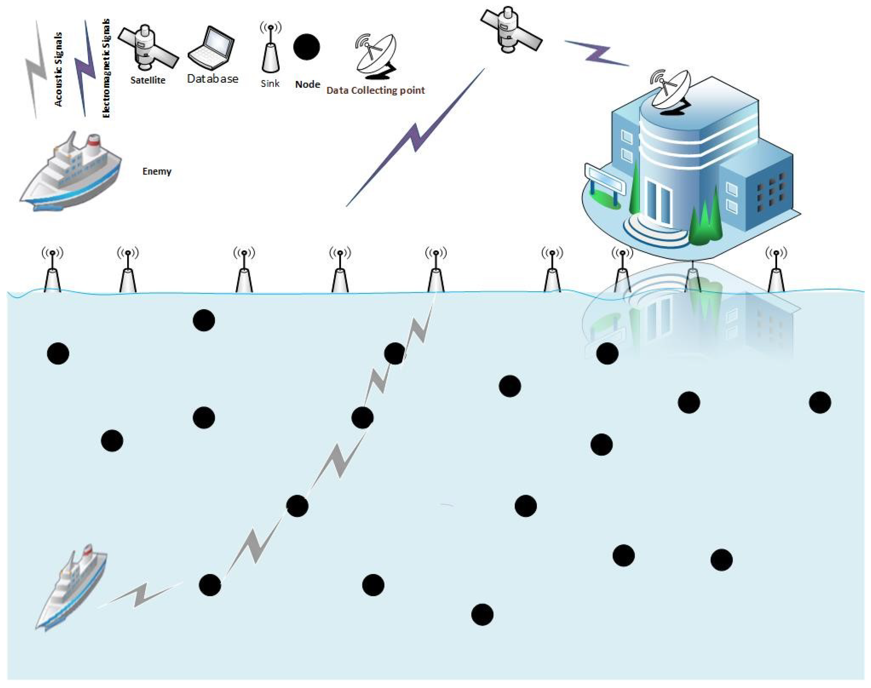
The network architecture of the ESEVBF protocol is composed of anchored nodes, relay nodes, and sink nodes, as depicted in Figure 1. The terminus nodes/sink nodes are centralized stations consisting of acoustic and radio modems. They communicate with each other and with the external network through the radio links. Sink nodes are fixed at the water surface. The data received by any sink node is considered to be a successful delivery to its destination. On the other hand, relay nodes are movable with the water current, while anchored nodes are fixed at the bottom. The sensor nodes communicate with each other through an acoustic link. The speed of the acoustic signal (1500 m/s) is much smaller than that of the electromagnetic signal ($3.8\times {10}^8$ m/s). Environmental monitoring and underwater tectonic plates monitoring are the typical applications of the network.

Timer Value Calculation Based on the Packet Advancement from the Source Node to the Second-Hop Potential Forwarding Node and on the Energy Tax Value in the Forwarding Region

The proposed protocol distinguishes between five distinct kinds of packets, which are Neighbor Request, Acknowledgment, Container, Announcement, and Data Packet. The sensor nodes are set up in the various locations. When the packet is ready to be forwarded, the timer mechanism is used to choose the next forwarder. The packet is transmitted by the source node to all of the potential forwarding nodes (PFNs), which then receive it. In the event that the PFN does not change its position at any point in the locality, then in the case of real life in the simulation, a single node will be chosen every time the source broadcasts the packet. Because of the repeated selection, the currently chosen node will enter a dead state after a certain amount of time has passed. Therefore, the sensor nodes move around and their positions change in a random pattern. These nodes are qualified to act as forwarding nodes if the current source node is shallower, and if the distance between them is closer together than the transmission distance. The Neighbor Request Packet is broadcast by the source node in order to locate the forwarding nodes that it needs. The Neighbor Request Packet has the format $N_{req}(id, d, Typ{e}_{packet})$, where id is an unchanging integer number that is specific to the sensors nodes, d is a field that was initially assigned to each node during the initialization phase, which stores information regarding the depth, while $Typ{e}_{packet}$ is a number in binary format that is used to distinguish each of the packets. As soon as a Neighbor Request Packet is received, the neighbor sends a Neighbor Acknowledgment Packet in response. In the configuration of an $Ac{k}_{packet}(id, d, residua{l}_{energy}, Typ{e}_{packet})$, id is a unique number that is given to each node, d is the data packet type, and $residua{l}_{energy}$ is residual energy or energy status and $Typ{e}_{packet}$ denotes the packet type, i.e., in the current case, it will denote an Acknowledgement Packet. At the first hop, the PFNs of the source node communicate with one another using packets through Container Packets, also known as CPs, to exchange their priorities. Whenever a data packet is delivered to a neighbor node from the source node, the neighbor node immediately calculates its own timer value, in addition to determining the bare minimum required timer for the second hop. The structure of a Container Packet can be described as $Can(id, Time{r}_{Hop1}, Time{r}_{Hop2}, Typ{e}_{packet})$, where id is the unique number of the sending node, $Time{r}_{Hop1}$, is the timer value at first hop, and $Time{r}_{Hop2}$ is the timer value at the second hop (the minimum timer value among the second-hop forwarder of the applicant adding $Time{r}_{Hop1}$ and $Typ{e}_{packet}$ represents the packet type, i.e., in this case, the container packet. When the source node is in possession of the Container packets sent by each of the Announcement Packets, it broadcasts to the neighbors (AC). This particular kind of packet is utilized in the process of the concealed and ultimately fatal problem, which will be covered later in this section. The Announcement Packet follows this format for its contents: $Announcemen{t}_{packet}=(i{d}_{\left(highes{t}_{priority}\right)}, x, y, z, Typ{e}_{packet})$, in which $i{d}_{\left(highes{t}_{priority}\right)}$,x, y, and z stand for the id and coordinates of the node with the highest priority; $Typ{e}_{packet}$ represents the type of packet, i.e., the announcement packet, in the current case; and the final type of packet is called a Data Packet, and it contains the actual data or information that must be transmitted to the centralized station. Data Packet refers to the format that Data Packet uses—$Dat{a}_{Packet}=(Header, Payload, Typ{e}_{packet})$. The header of the packet includes information regarding the node that generated the packet, as well as the centralized station. The payload of the data packet is the most important component, as it contains the data that actually pertains to the environment, and $Typ{e}_{packet}$ represents the packet type. In the event that the preceding packets of data are transmitted at frequent but brief intervals, then increased network overhead and power consumption can be anticipated. Because of this, in order to circumvent this issue, every node maintains its own corresponding neighbor table, for the purpose of keeping a record of their fellow community members: $Neighbo{r}_{table}=(id, residua{l}_{energy}, d, Time{r}_{value},Updat{e}_{time})$, where id is neighbor node unique number, $residua{l}_{energy}$ is the residual energy of the node, d represents the Depth information, $Time{r}_{value}$ is the timer value of the node, and $Updat{e}_{time}$ stands for the time required to update the neighbor entry. In the meantime, when there is sufficient time for the neighboring nodes to be updated, the source node will send out and receive the second packet. Then, the source will immediately broadcast the Data Packet, as well as the Announcement Packet that was contained in the prior table.

4. Timer Value Methodology of a Forwarder Node for the Proposed Scheme

The source broadcasts the packets to its neighbors in its transmission range. All of the nodes lying in the transmission range of a source node will receive the packet. If all the neighbor nodes of a source node take part in broadcasting, then there will be a higher packet overhead, and this will result in higher energy consumption. Therefore, to minimize the broadcasting of a forwarder of source nodes, the timer value calculation mechanism is investigated. Upon the reception of the packet from the source node, the potential forwarding nodes first checks the depth information of the source node. The potential forwarder starts working to calculate the time value if its locality is above the source nodes, or else it drops the packet. The timer value is calculated based on the fitness function value. DO-WPR only considered the depths of the first and second hops, and did not consider the residual energies of the nodes in the forwarding region of the forwarder node. From Figure 1, the source node S broadcasts the packet, while all its neighbors, i.e., A, B, C, N, and M, in its transmission range, receive the packet. The forwarding nodes A, B, and C are the eligible nodes for further broadcasting the packet to the centralized station, while N and M have higher depth than the source node; therefore, it will drop the packet, as A, B, and C are the eligible nodes for further forwarding the packet. If all the three nodes forward the packet, then this will result in a higher overhead and energy consumption. Upon the reception of the packet, A, B, and C will calculate the timer value. The timer value for the corresponding node will decide its priority of transmission; the lesser the timer value, the higher its priority of transmission. The timer value is calculated based on the packet advancement from the source node to the second-hop potential forwarding node, and on the energy tax value in the forwarding region. When anyone between the three nodes transmits the packet, then the other two nodes, if they are in the transmission range, will receive the copy of the packet. When the nodes receive the copy of the packet, it will drop the packet, suggesting that some other node having a higher priority of transmission has already transmitted the packet.

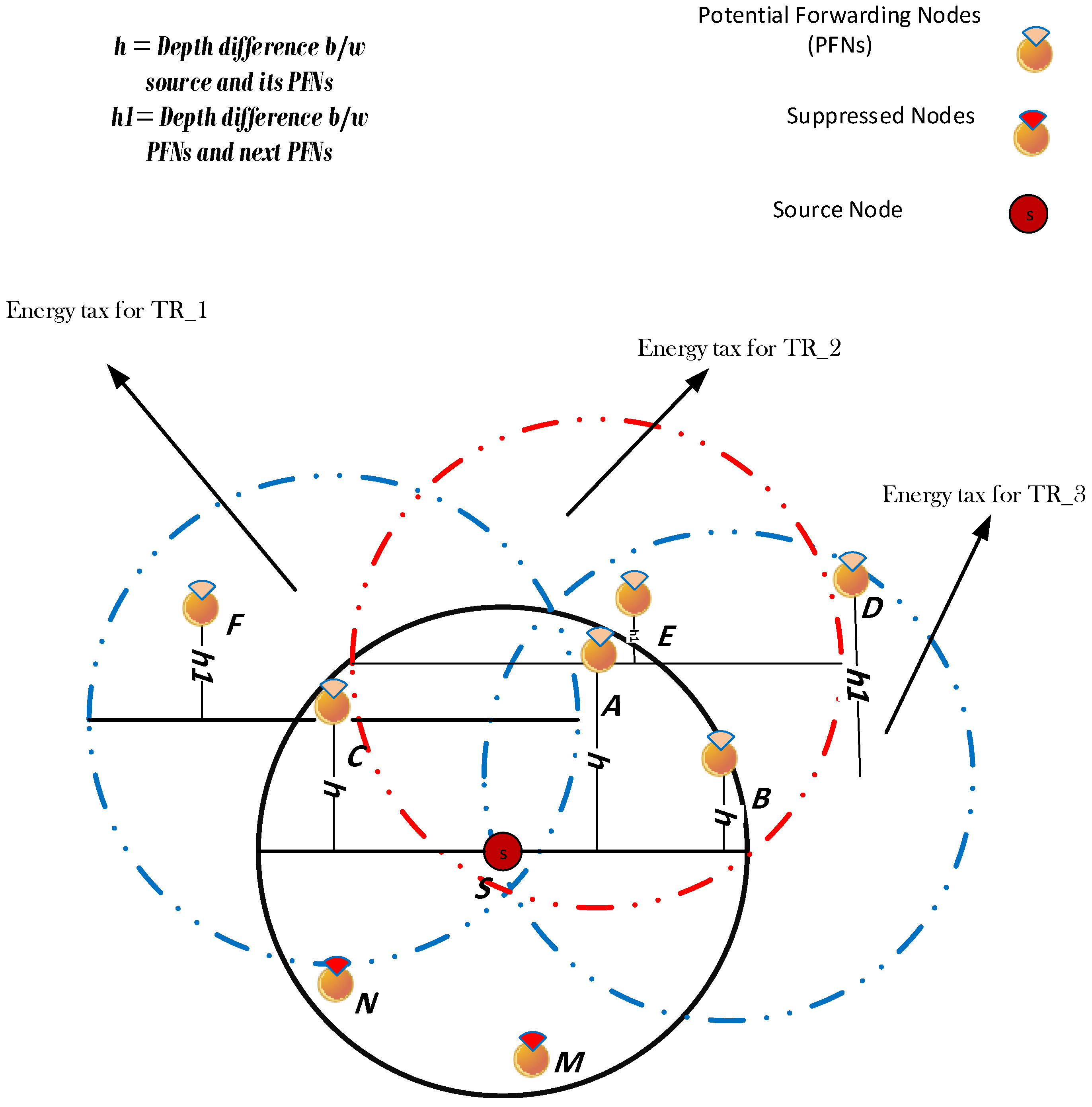
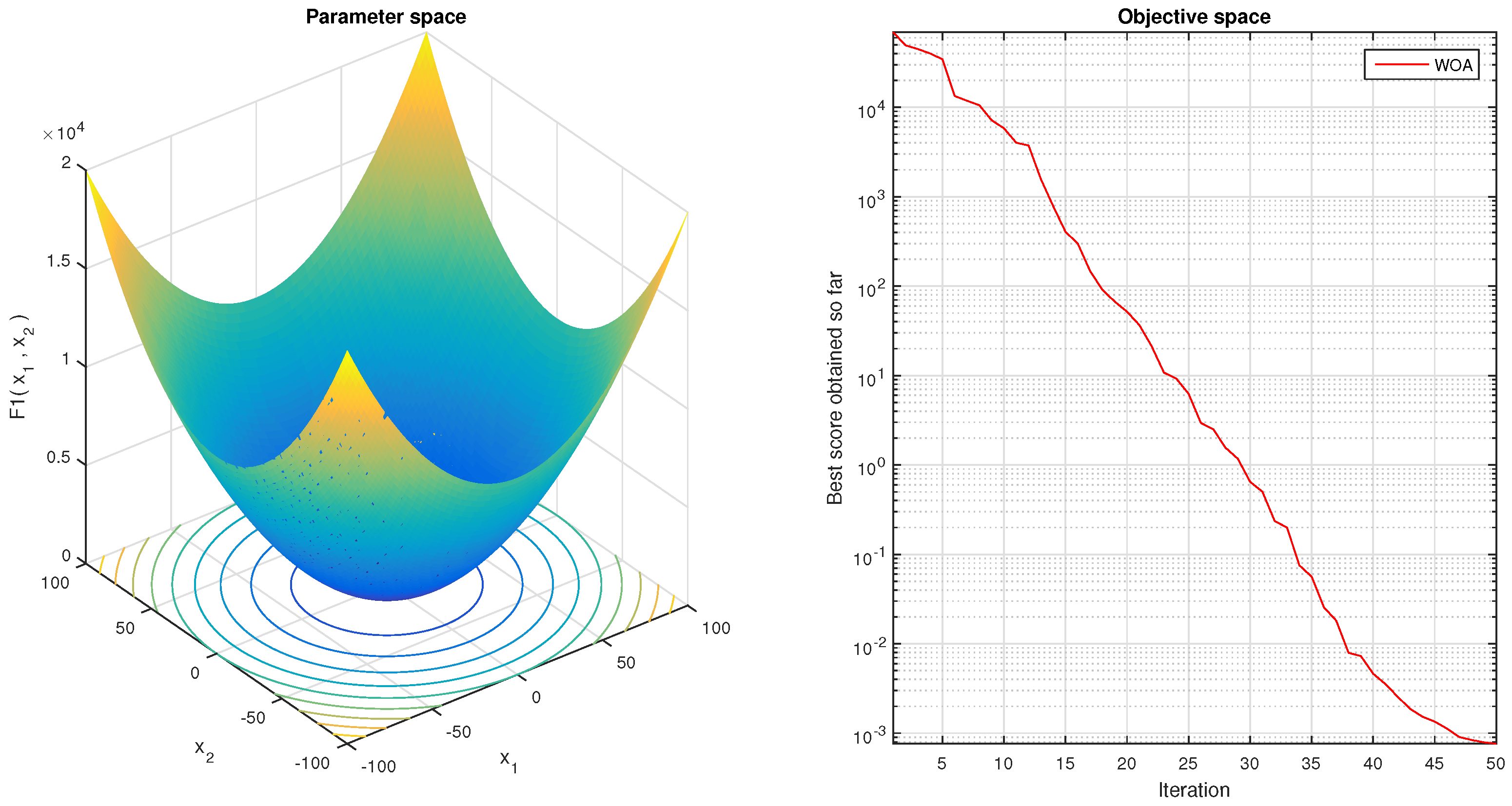
The proposed work uses the Whale Optimization Technique (WOA) to find the energy tax value for the forwarding region, and based on this value, the network forwards in the direction where there is a higher value of the energy tax illustrated in Figure 2. The proposed work will calculated the fitness function value of the proposed work ($F{F}_{BDREA}$), considering the parameters related to the potential forwarding nodes of the source nodes, i.e., the packet advancement in two hops (H), the number of potential forwarders and suppressed nodes below the source nodes, i.e., $PF{N}_{num}$ and $SU{P}_{num}$, respectively, the number of hops from the sink nodes to the source node, and the energy tax in the locality of forwarding node that is most in favor of performance metrics. Thus, the proposed scheme will consider all of the above mentioned.

To find the fitness function of the BDREA ($F{F}_{BDREA}$) value, the potential forwarders and suppressed nodes metrics are considered from set 3 of DOW-PR, while the energy tax is found with the help of WOA. The proposed algorithm uses the Whale Optimization Algorithm (WOA) technique to find the optimum number of PFNs of forwarder nodes with the best energy normalization value in the network, based on the following function, as shown in Equation (1).

$$E_{tax}=\frac{E_{total}}{ForwardingNodes\times Dat{a}_{Packets}}$$

(1)

where $E_{total}$ is the total energy constrained in a transmission range of the forwarding nodes, nodes are the number of potential forwarding nodes in the transmission range of a forwarder nodes, and packets are the numbers of data packets to be delivered from the forwarding region.

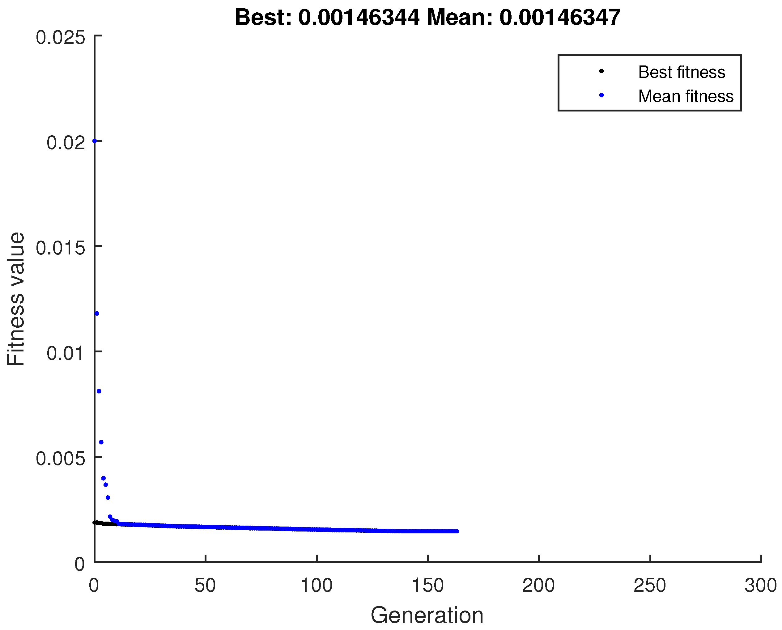
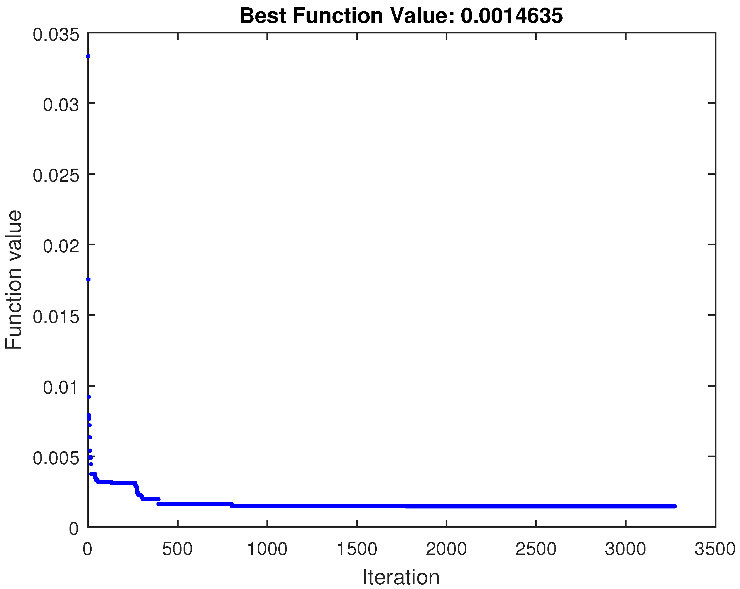
The researcher faces a huge issue in balancing the energy consumption of nodes that are responsible for routing data from source to destination. Maximum end-to-end delay, multipath fading, and mobility issues are among the most challenging issues for UWSNs. Nodes utilized solely to transport data packets are referred to as “courier or relay nodes,” and the optimal cost function for weight computations is used to balance the energy consumption of sensor nodes. As an additional benefit, good coordination between nodes can help reduce energy use. Static or mobile sinks are options for data collection structures. When using static methods, nodes that are closest to the sink use up their energy more quickly, and as a result, a segment or the entire network may become disconnected. Researchers are interested in UWSNs because of the enormous challenges they pose, and because of the unpredictable and harsh nature of water. It is possible to improve the network’s performance through a variety of protocols, including energy optimization, packet ratio, end-to-end delay, and so on. However, enhancing one network aspect can have an impact on other factors because each factor is linked in some way. After further discussion, it is clear that if we wish to improve packet delivery ratio, it has an impact on the energy tax of protocols, and hence the network’s throughput. 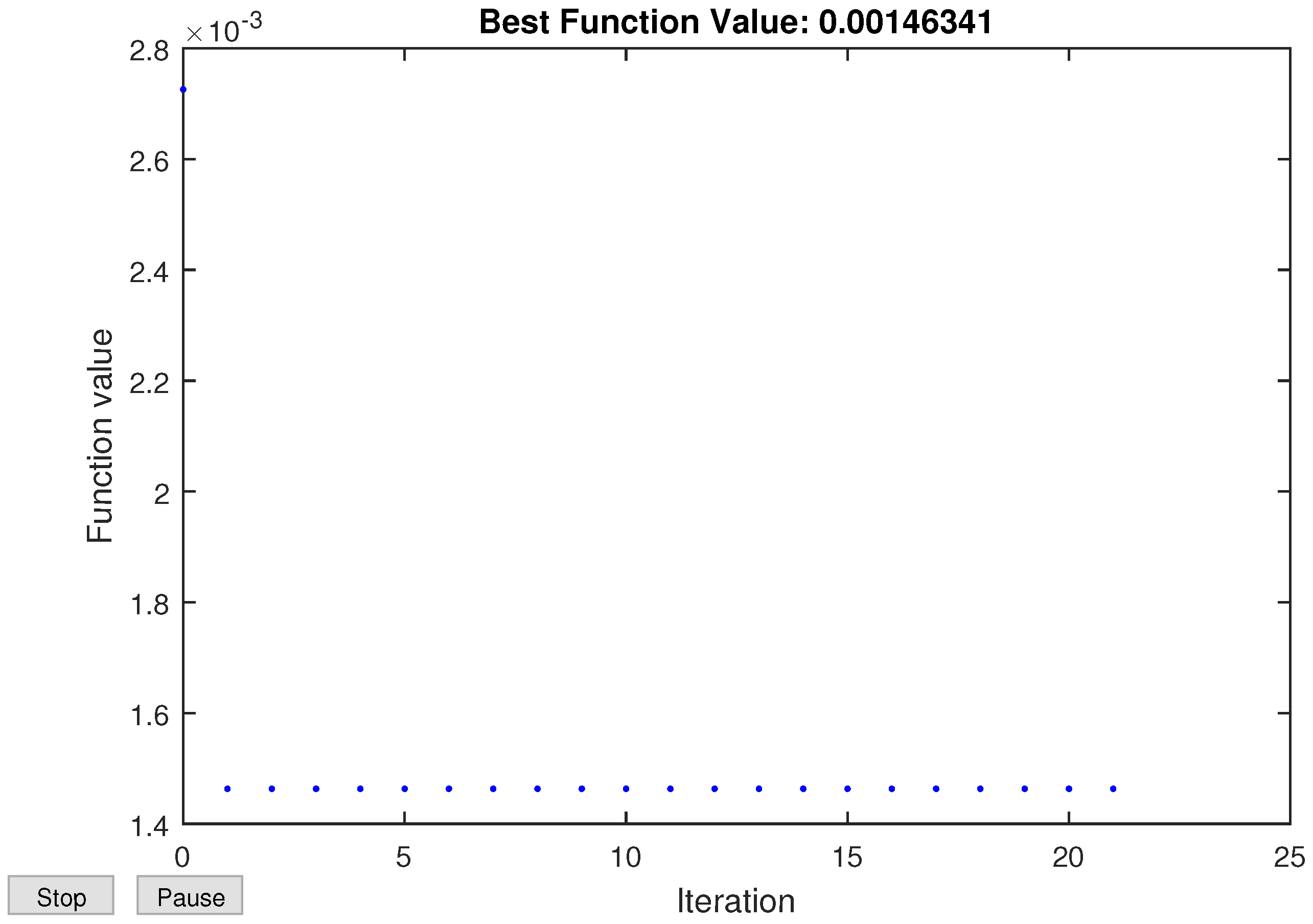The objective function has been also optimized with the help of different optimization algorithms, including Genetic Algorithm (GA), Simulated Annealing (SA), Particle Swarm Optimization (PSO), and Whale Optimization algorithm (WOA), as shown in Figure 3, Figure 4, Figure 5 and Figure 6. The purpose of the objective function is to reduce the total energy consumption.

The results represent the fitness function value against iterations. All the algorithms are working to find the best function value for the objective function (Energy tax). This means that to find the best value for energy tax function, the network will perform optimum aligning with the lower and upper bound requirements. In the lower and upper bounds, the total energy and number of nodes are specified for deployment and for the total number of packets to be successfully received from a specific transmission of the source node. For lower iterations, WOA is reached to find the best minimum value compared to GA, SA, and PSO.

The fitness function of DOW-PR can be further enhanced by using the energy tax value of the forwarding locality, i.e., the fitness function value of BDREA can be calculated as given below in Equation (2):

$$F{F}_{BDREA}=\frac{H}{DI{V}_{PFN}+DI{V}_{SUP}\times Hop\_to\_sink}\times e^{-(E_{tax}/E_{residual})}$$

(2)

where H is the fitness function value of DOW-PR, which contains the advancement from the source node to its expected next potential forwarding, $DI{V}_{PFN}$ and $DI{V}_{SUP}$ is the factor of the potential forwarding nodes and suppressed nodes from set 3, correspondingly, $HOP\_to\_sink$ is the number of hops from the surface sink to the forwarding nodes, and $E_{tax}$ is the amount of energy constrained within the forwarding zone as from Equation (1), while $E_{residual}$ is the total residual energies in the network. The timer value is the function of the fitness function value of $F{F}_{BDREA}$:

$$F{F}_{BDREA}=k\times \left(F{F}_{BDREA}\right)+\beta$$

(3)

$$F{F}_{BDREA}=k\times \frac{H}{DI{V}_{PFN}+DI{V}_{SUP}\times Hop\_to\_sink}\times e^{-(E_{tax}/E_{residual})}+\beta$$

(4)

If the fitness value (H) for node A is greater than node B, then the following condition should be satisfied:

$$T\left(F{F}_{(BDREA\_A)}\right)<T\left(F{F}_{(BDREA\_B)}\right)$$

(5)

The holding time between two neighboring nodes should be different in such a way that the forwarder node that has a greater fitness function $\left(T\left(F{F}_{\left(BDREA\right)}\right)\right)$ value transmits the packet before the transmission of the same packet from other nodes. For instance, if node A has the highest fitness function value, then it will transmit prior to node B. Upon receiving a duplicate packet from node A, it simply drops the packet. The following equation must be satisfied to avoid duplicate packets:

$$t_1+T\left(F{F}_{(BDREA\_A)}\right)<t_2+T\left(F{F}_{\left(BDRE{A}_B\right)}\right)+t_{12}$$

(6)

Substituting Equation (3) in Equation (6) results in:

$$k\le \frac{(t_2-t_1)-t_{12}}{F{F}_{BDREA\_A}-F{F}_{BDREA\_B}}$$

(7)

if we replace the $F{F}_{BDREA\_A}-F{F}_{BDREA\_B}$ with a global variable $\sigma$, as in DOW-PR.

$$k\le \frac{(t_2-t_1)-t_{12}}{\sigma }$$

(8)

Solving the value of k and putting it in the above equation, then the timer value can be calculated as given below:

$$T\left(F{F}_{BDREA}\right)=\frac{\frac{2R}{V_0}}{\delta }\left(R-F{F}_{BDREA}\right)$$

(9)

The sensor nodes are set up in the various locations. When the packet is ready to be forwarded, the timer mechanism is used to choose the next forwarder. The packet is transmitted by the source node to all of the potential forwarding nodes (PFNs), which then receive it. In the event that the PFN does not change its position at any point in the locality, then in the case of real life, in the simulation, a single node will be chosen every time the source broadcasts the packet. Because of the repeated selection, the currently chosen node will enter a dead state after a certain amount of time has passed. Therefore, the sensor nodes move around and their positions change in a random pattern. These nodes are qualified to act as forwarding nodes if the current source node is shallower, and if the distance between them is closer together than the transmission distance. The Neighbor Request Packet is broadcast by the source node in order to locate the forwarding nodes that it needs. To determine which is the best next hop, every node maintains its own corresponding neighbor table, which is for the for the purpose of keeping a record of their fellow community members: $Neighbo{r}_{table}(id, residua{l}_{energy}, d, Time{r}_{value},Updat{e}_{time})$, where id is the neighbor node unique number, $residua{l}_{energy}$ is the residual energy of the node, d represents the Depth information, $Time{r}_{value}$ is the timer value of the node, and $Updat{e}_{time}$ stands for the time required to update the neighbor entry.

Algorithm1: Algorithm BDREA for selecting the Next forwarder among potential forwarding nodes.

5. Simulation Results and Analysis

The proposed work is simulated against different parameters, i.e., packet delivery ratio (PDR), end-to-end delay, Average Accumulated Propagation Distance (APD), and energy tax. Packet Delivery Ratio (PDR) is defined as the ratio of the successful transmission of packets from the source node to the destination node that is the sink or centralized station. PDR can be expressed with the following equation:

$$PDR=\frac{Packet{s}_{received}}{Packet{s}_{sent}}$$

(10)

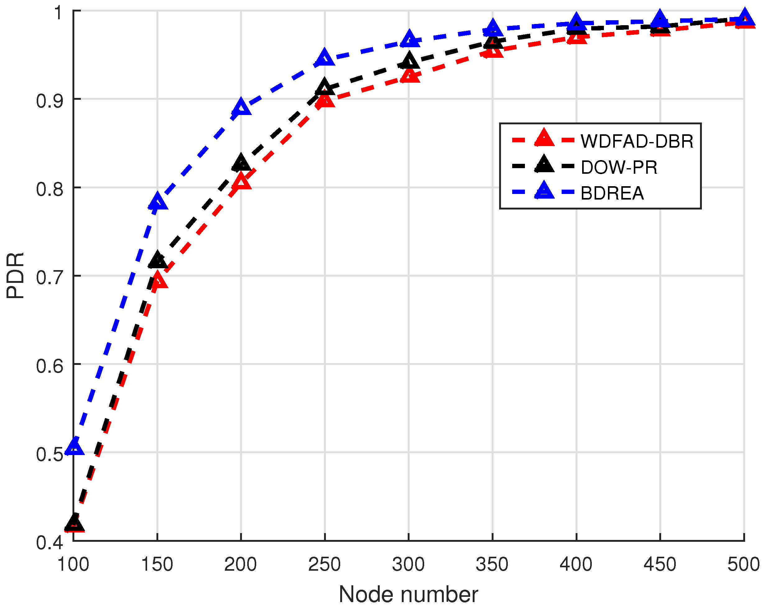
The results of PDR for the proposed work (BDREA) are plotted against the DBR, WDFAD-DBR, and DOW-PR routing protocols, as shown in Figure 7. The results are obtained by varying the total number of nodes in the network, ranging from 100 to 500 nodes. There is an increasing trend in PDR when increasing the number of nodes in the network. This is due to the fact that by increasing the number of nodes in the network, it also increases successful delivery to its destination, i.e., lowering the probability of packets dropped. As from Figure 7, for 100 nodes in the network, the PDR is approximately 40%, which shows a higher probability of packets dropped for the WDFAD-DBR and DOW-PR protocols.

PDR is gradually increased by increasing the number of nodes in the network, and for about 500 nodes, it approaches the highest peak PDR values with the aid of a higher packet overhead and a higher total energy consumption. WDFAD-DBR and DOW-PR consider the total packet advancement at the first and second hops. Therefore, by considering the first- and second-hop potential forwarding nodes of the source node, WDFAD-DBR and DOW-PR reduce the packets dropped probability and show a higher PDR—refer to Figure 7. Our proposed BDREA routing protocol not only considers the packet advancement over the first two hops from the source node, the traffic congestion, and the distance from to the surface station, but it also considers the inverse normalized energy tax values of the potential forwarding zones of the source nodes, and therefore, balances the total energy in the network. The number of alive nodes for the BDREA protocol is higher, by balancing the energy in the network, which means that a finding a suitable node with respect to the timer value will mostly occur. Therefore, the BDREA routing protocol reduces the packet dropped ratio while maintaining a higher PDR value, as from Figure 3. The timer value calculation is the major factor for improving the related objective parameters, by tuning the related metrics. The objective of this article is to improve the related parameters by considering the energies of the potential forwarding nodes in the forwarding locality. This will prolong the network life, and at each instance of time, more favorable forwarding nodes will be available for selecting the next forwarding. BDREA defeats the benchmark, DOW-PR, by an average of 8% improved PDR, and WDFAD-DBR by 10% improved PDR for the 200 nodes in the network.

The total energy consumption is defined as the average energy consumed per node during the successful transfer of the packet from the source node to a sink node. It includes the sending, receiving, and idle state energy. The computation equation is the following:

$$Energ{y}_{tax}=\frac{E_{total}}{Nodes\times Packets}$$

(11)

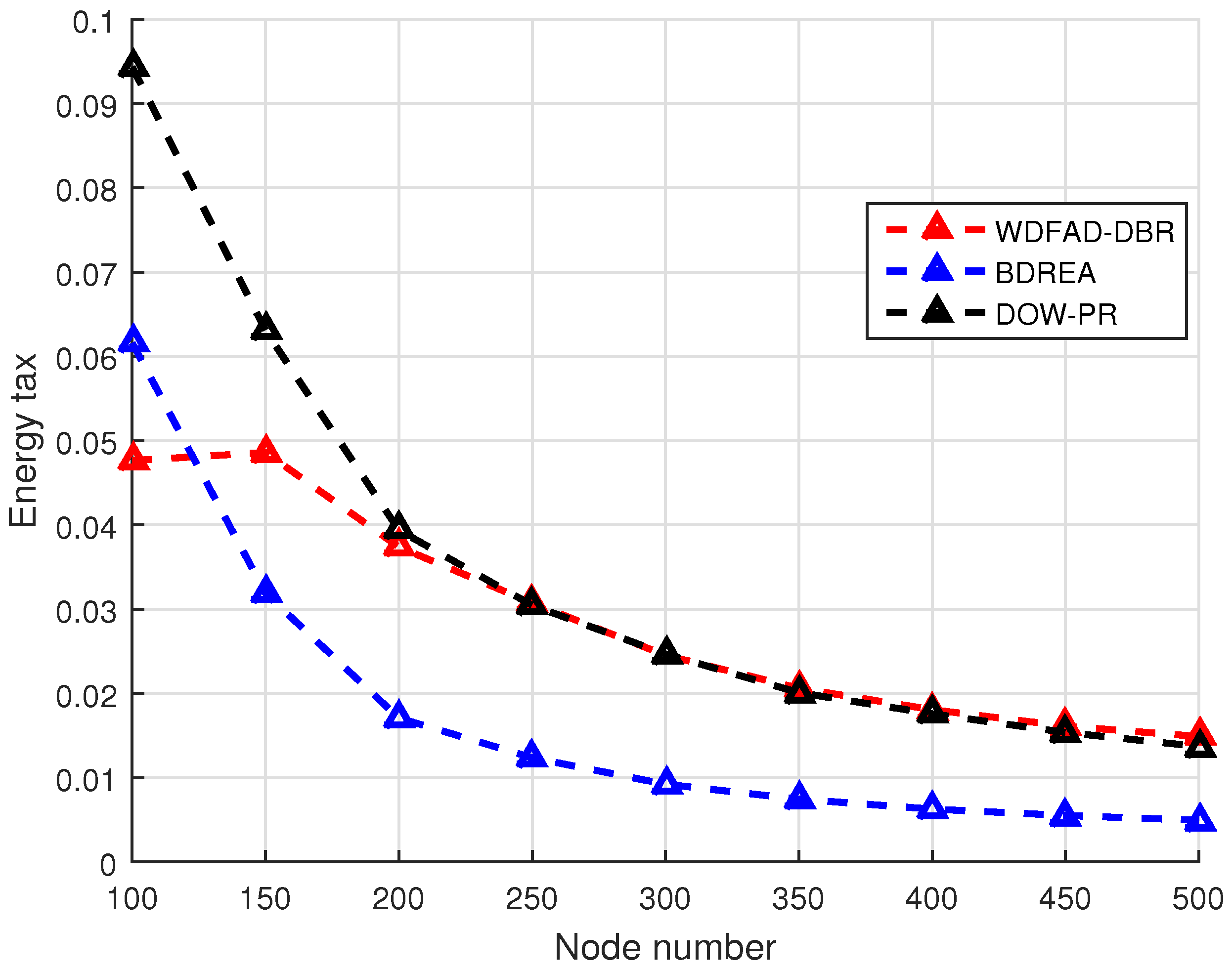
where $E_{total}$ denotes the whole network energy, and Nodes and Packets denote the number of nodes and packets successfully received, respectively. The energy tax for the all of the schemes is plotted by varying the number of nodes in the network, as shown in Figure 8. The general trend followed by all of the protocols is that the energy tax decreases when the number of nodes in the network is increased. For a node number of 100, the performance of the proposed work for BDREA in terms of energy tax is lower than in the conventional schemes. This is due to the fact that the conventional schemes find better nodes in terms of packet advancement, while there exists a minimum packet overhead, due to a less dense network. The performance of BDREA is better for a dense network, to save energy utilization in terms of packet overheads, and in exchanging the different packets. It can be visualized that the proposed BDREA defeats the other protocols in terms of energy tax for a dense network. This is due to the fact that the proposed work considers the energy of the forwarding zones in forwarding the packets, which balances the overall residual energies of the nodes in the network; therefore, it prolongs the network life time. For each packet transmission, the network will find the best suitable nodes in terms of the timer value parameter, and will optimize the energy performance. It can be seen from Figure 4 that the proposed work improved the energy tax of the network by approximately 50%, compared to DOW-PR and WDFAD-DBR.

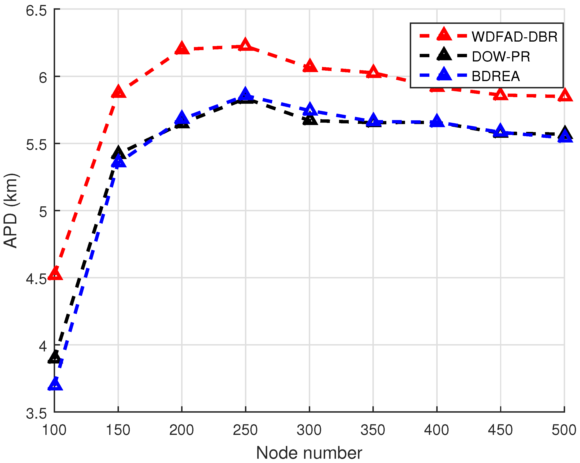
The Average Accumulated Propagation Distance is the distance covered by each packet during the hop-to-hop transmission. Actually, it is the hop distance that is measured. As there are many sink nodes in a network, so the packet distance to the shortest sink is measured as the final accumulated propagation distance. The equation of APD is defined as follows:

$$APD=\frac{1}{s}\sum _{j=1}^s\sum _{i=1}^k\mathrm{dist}{}_i^j\mid$$

(12)

where the number of packets successfully delivered, and the hop number from the source to sink node is represented by s and k, respectively; $dis{t}_i^j$ is the propagation distance of the ith hop of the jth packet. APD is plotted for all the protocols in Figure 9. It can be seen from the results that DOW-PR and BDREA result in the same APD values, because both the protocols consider the distance to the surface station and the number of hops up to the centralized station.

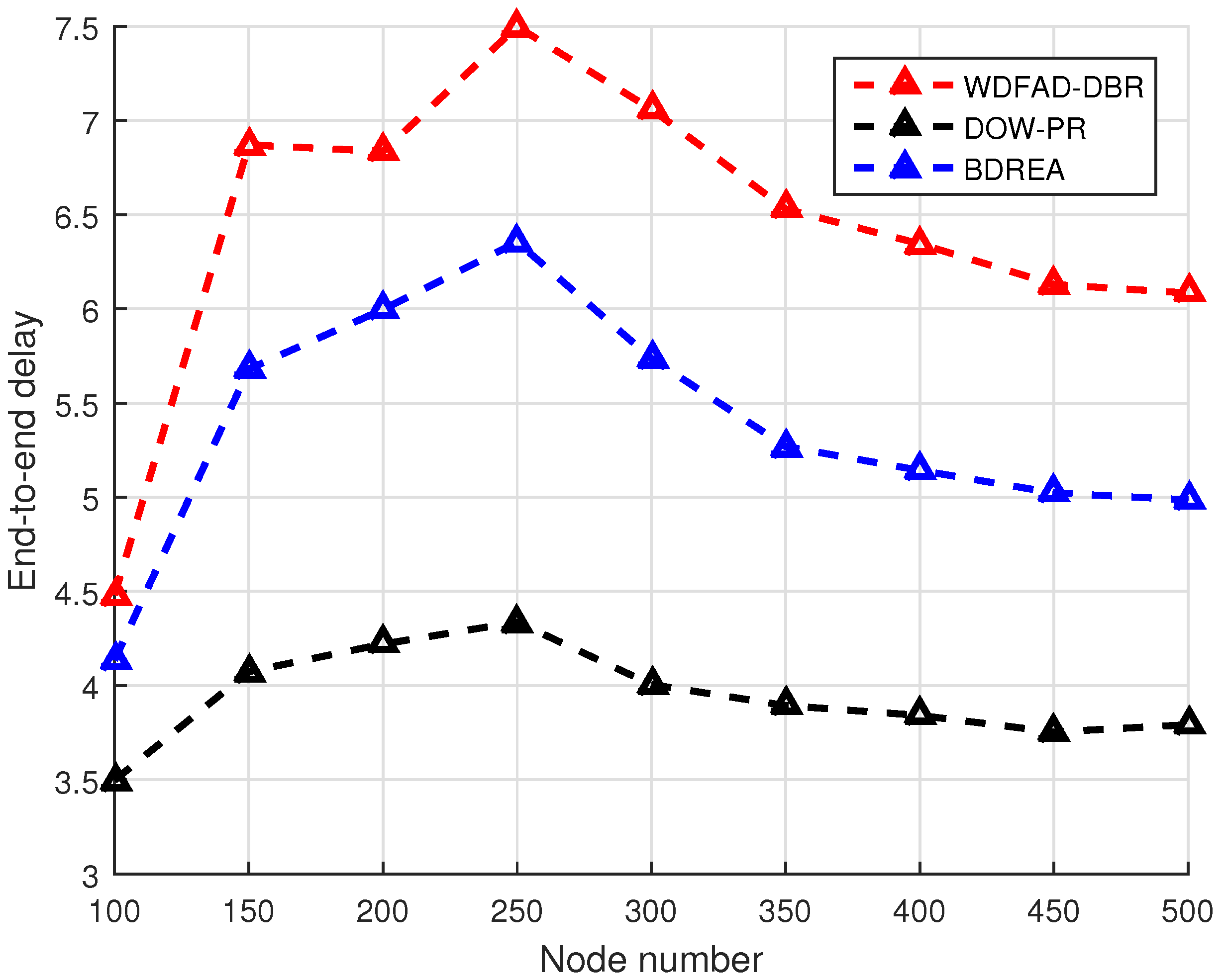
End-to-End delay is another important parameter that is defined as the total time taken by a packet to travel from the source node to the sink node. This includes the transmission time delay, the holding time delay, and the propagation time delays. The end-to-end delay curve is plotted in Figure 6 for WDFAD-DBR, DOW-PR, and BDREA. DOW-PR reduces the end-to-end delay time and improves the performance by 15% illustrated in Figure 10, compared to the proposed work’s BDREA. The fact can be verified from the timer calculation equation and the fitness value equation that the BDREA is more focused towards energy minimization, which also results in enhanced PDR. For the instance of time, if there exist two paths for transmission, BDREA will prioritize the one where the least amount of energy is consumed, while DOW-PR will prioritize the one where an end-to-end delay results in a minimum time. BDREA results in an 18% reduction in end-to-end delay when compared with WDFA-DBR, as BDREA also considers the distance to the surface sink in selecting the next forwarder, and therefore reduces the end-to-end delay time. Comparing BDREA with WDFAD-DBR, it improves the results by 5% and therefore results in a lower end-to-end delay.

6. Conclusions

A novel Betta and Dolphin Pods Routing and Energy Scarcity Aware (BDREA) protocol has been developed for an underwater wireless sensors network. The sensors are producing and transmitting data packets in their immediate area, while the nodes in their neighbors’ networks are receiving the packets. The nodes that belong to the neighbors have the ability to act as forwarding nodes, which means that they can send data packets onwards toward centralized stations. A timer mechanism is calculated in order to prevent packets from being overheard, and to reduce the amount of energy that is consumed. The computation of the timer used by BDREA takes into account the progression of the packets during the first two hops after the source node, the volume of traffic along the forwarding path, the distance to the centralized station, and the inverse energy of the forwarding region. When compared to the benchmarks WDFAD-DBR and DOW-PR, the work that was presented had a better performance in terms of PDR, energy tax, and end-to-end latency. To be more exact, it has been determined that BDREA improves PDR by 8%, energy tax by 50% in comparison to DOW-PR, end-to-end delay by 18%, and APD by 5%, in comparison to WDFAD-DBR.