Abstract
This paper delves into an in-depth exploration of speaker recognition methodologies, with a primary focus on three pivotal approaches: feature-level fusion, dimension reduction employing principal component analysis (PCA) and independent component analysis (ICA), and feature optimization through a genetic algorithm (GA) and the marine predator algorithm (MPA). This study conducts comprehensive experiments across diverse speech datasets characterized by varying noise levels and speaker counts. Impressively, the research yields exceptional results across different datasets and classifiers. For instance, on the TIMIT babble noise dataset (120 speakers), feature fusion achieves a remarkable speaker identification accuracy of 92.7%, while various feature optimization techniques combined with K nearest neighbor (KNN) and linear discriminant (LD) classifiers result in a speaker verification equal error rate (SV EER) of 0.7%. Notably, this study achieves a speaker identification accuracy of 93.5% and SV EER of 0.13% on the TIMIT babble noise dataset (630 speakers) using a KNN classifier with feature optimization. On the TIMIT white noise dataset (120 and 630 speakers), speaker identification accuracies of 93.3% and 83.5%, along with SV EER values of 0.58% and 0.13%, respectively, were attained utilizing PCA dimension reduction and feature optimization techniques (PCA-MPA) with KNN classifiers. Furthermore, on the voxceleb1 dataset, PCA-MPA feature optimization with KNN classifiers achieves a speaker identification accuracy of 95.2% and an SV EER of 1.8%. These findings underscore the significant enhancement in computational speed and speaker recognition performance facilitated by feature optimization strategies.
1. Introduction
This paper introduces an expansion of our earlier work on speaker recognition (SR) systems, concentrating on the methodology of feature-level fusion across various sizes of voice data [1]. Our previous paper proposed an innovative approach to enhance speaker recognition rates by fusing diverse speech features. The model combined 18 different features, including the mel-frequency cepstral coefficient (MFCC), linear predictive coding (LPC), perceptual linear prediction (PLP), root mean square (RMS), centroid, and entropy features, along with their corresponding delta (Δ) and delta–delta (ΔΔ) feature vectors. The experimental results demonstrated that fusing various features with their corresponding delta and delta–delta values can lead to a significant increase in speaker identification accuracy, showing improvements ranging from 10% to 50% on clean voice data using linear discriminant (LD), K nearest neighbor (KNN) and ensemble classifiers. Additionally, the equal error rate (EER) value for speaker verification was reduced compared to using a single feature.
While combining many features may seem beneficial for capturing diverse aspects of the data, it can also introduce several challenges associated with the curse of dimensionality, including increased computational complexity, overfitting, and diminished performance. Balancing the number of features with the desired performance and computational constraints is crucial in designing effective speaker recognition systems. To overcome this challenge, dimension reduction techniques, such as principal component analysis (PCA) and independent component analysis (ICA), and feature optimization techniques are employed. These techniques compress data by reducing the dimensionality while preserving the most important features. Consequently, the training process is accelerated, leading to improved computational efficiency [2,3].
Furthermore, this paper introduces feature optimization methods, including genetic algorithms (GAs) and marine predator algorithms (MPAs), to select the best features for speaker recognition systems with dimension reduction techniques. These algorithms help identify the most informative and discriminative features, enhancing the overall performance of the system. Moreover, optimization methods often mitigate the curse of dimensionality by reducing feature dimensionality while preserving relevant information, leading to more efficient processing and better generalization across different speakers and speaking conditions. Additionally, feature optimization techniques facilitate adaptation to speaker variability and integration with machine learning models, resulting in improved recognition accuracy and reliability [3,4,5,6].
The main contributions of this paper are as follows.
- We have thoroughly investigated a range of dimension reduction techniques and feature optimization methods specifically designed to tackle the complexities of high-dimensional data within speaker recognition systems.
- Overall, the research emphasizes the significance of feature optimization in speaker recognition systems and highlights the advantages of feature fusion, dimension reduction, and feature optimization techniques.
- The objective is to find the optimal combination of features that not only improves recognition accuracy but also reduces the dimensionality of the feature space, leading to faster computation.
- Our proposed models present robust solutions for improving speaker recognition performance in noisy environments across datasets of various sizes, accommodating different numbers of speakers. From small datasets with 120 speakers to medium ones with 630 speakers and large ones with 1251 speakers, our models demonstrate versatility, making them suitable for a broad range of applications and datasets with diverse scales and characteristics.
This paper is organized into distinct sections to ensure a comprehensive presentation of the research. In Section 2, the related work offers a comprehensive overview of previous research on automatic speaker recognition systems. Section 3 describes the proposed work and methodology and delves into the theoretical and practical aspects of our novel approach. In Section 4, which presents database descriptions and an evaluation of the results, we explore the databases used and analyze the performance parameters. In Section 5, the results are discussed, and we conduct a thorough comparison between the proposed results and those of existing methods. Finally, Section 6 succinctly summarizes the findings.
2. Related Work
In this section, we provide a summary of research related to speaker recognition, focusing particularly on the noisy TIMIT and voxceleb1 databases. The study in [2] considered dimension reduction in speaker identification using mutual information, underscoring the importance of selecting informative features and discarding irrelevant features to enhance the efficiency of speaker recognition systems. The studies in [3,4] proposed feature selection and dimensionality reduction techniques that employed GAs for speaker recognition; the aim was to improve accuracy and computational efficiency and reduce the dimensionality of the feature space.
The study in [5] offered a comprehensive survey on the MPA, emphasizing the significance of feature optimization across various domains; although, this study was not directly centered around speaker recognition. In [6], an efficient MPA was introduced for feature selection, contributing to the advancement of feature selection techniques and their applications in various domains. The study in [7] employed a deep neural network (DNN) for the extraction of bottleneck features. The concatenation of MFCC and linear prediction cepstrum coefficient (LPCC) features was utilized in [8] to enhance speaker identification results.
In [9], a method combining feature selection and feature merging based on learning from multiple kernels was proposed; it ultimately improved the performance of speaker recognition systems. The concatenation of acoustic features from multiple channels was explored to enhance speech recognition in [10]. While feature fusion through concatenation can boost performance, the associated increase in dimensionality was acknowledged as a drawback, which can be mitigated by dimension reduction techniques [11,12].
Delta and delta–delta function values were incorporated to offer extra statistics and detect function variations over small periods of speech [13]. Dynamic features, introduced by Furui [14], were used to capture temporal variability in feature vectors. To address the overall performance degradation of popular computerized speech (automatic speaker recognition) systems in the presence of additive noise, numerous techniques along with statistical version edition, noise reduction techniques, and noise-resistant functions have been proposed. Techniques such as spectral subtraction, RASTA, and lin-log RASTA [15,16,17,18,19,20,21,22] have been considered for improving the robustness of cepstral approaches to noise.
Research papers [23,24,25,26] have showcased the substantial enhancement in speaker recognition system performance achieved through the utilization of delta values and prosodic information. Within a biometric system, feature-level fusion and score-level fusion have been recognized as essential fusion levels [27,28]. Feature-level fusion, in particular, offers more information compared to a single feature, thereby augmenting the performance of speaker recognition systems [28]. The application of information theory to speaker recognition systems was explored in [29,30], and it has been demonstrated that the fusion of various speech features contributes to the improvement in speaker recognition system performance [31].
MFCC features, which are based on psychoacoustic theory [32], have been widely used in speaker recognition systems. The i-vector speaker recognition system, introduced by Dehak et al. [33], heavily relies on MFCCs as the primary source of speech features. PCA can be executed using techniques such as singular value decomposition (SVD), and iterative PCA methods have been identified as more accurate and efficient for the identification of dominant eigenvectors [34]. Expectation maximization (EM) and power iteration techniques have also been employed to enhance PCA [35,36]. Statistical cues, PCA, and ICA have been explored within the realm of speaker recognition systems [37,38,39,40].
In [41], the use of genetic programming (GP) for feature selection in speaker verification systems was introduced. The score fusion technique was proposed in [42] for speaker identification (SI) systems, and its performance with and without the addition of nonstationary noise (NSN) and white gaussian noise (AWGN) was evaluated, and features, including MFCCs and power-normalized cepstral coefficients (PNCCs) with GMM-UBM acoustic modeling were explored. In [43], the difference between the i-vector and GMM-UBM models was highlighted using clean and noisy speech from TIMIT and NIST-2008 speech records.
In [44], a mathematical derivation demonstrated that ICA can enhance feature representations for non-gaussian signals. A comparative study presented in [45] analyzed MFCC, IMFCC, LFCC, and PNCC speech features using a gaussian mixture model (GMM) under both clean and noisy speech conditions. In [46], a novel feature for speaker verification was proposed; it leveraged the advantages of low-variance multitaper short-term spectral estimators and the acoustic robustness of gammatone filterbanks.
The study described in [47] considered text-independent speaker verification by employing x-vector and i-vector approaches and utilizing the voxceleb1 and NIST-2012 voice datasets. In [48], an entirely automated pipeline that leveraged computer vision techniques was employed to create voxceleb1 data from open-source media. Investigating voice impersonation attacks and their implications for automatic speaker verification (ASV) systems was the central focus of the paper in [49]. Furthermore, the research paper in [50] thoroughly examined the encoding layers and loss functions utilized in end-to-end speaker and language recognition systems.
3. Proposed Approach and Methodological Framework
3.1. Motivation
Our primary objective is to pinpoint the most effective set of features that enhance accuracy, reduce error rates, and facilitate efficient computation, thereby conserving computational resources. Additionally, we aim to devise a universal approach applicable across small, medium, and large datasets, employing datasets with varying numbers of speakers for comprehensive analysis. This is the reason we have used different sizes of data in our work. Furthermore, this study delves into the impact of utilizing larger and more complex datasets, such as voxceleb1, on speaker recognition performance. In the domain of speaker recognition, research into computational timing has been relatively limited. Our proposed work fills this void by offering detailed insights into computational timing, a critical factor alongside accuracy and error rate. To realize this objective, we introduce three distinct approaches for speaker recognition (SR).
- Feature fusion Methodology: Feature fusion, a method that amalgamates features from diverse sources or databases into a unified, enriched feature set, stands as a pivotal strategy in speaker recognition systems. Spectral features, which encapsulate frequency, power, and other signal characteristics like MFCC, LPC, PLP, centroid, and entropy, provide a robust foundation. Conversely, prosodic features capture auditory properties such as stress, loudness variation, and intonation (e.g., RMS). While spectral features, particularly MFCC, have demonstrated superior performance compared to prosody-based systems (e.g., pitch, RMS), their combined integration offers unparalleled robustness vital for recognition systems. Additionally, feature derivatives enable the quantification of subtle changes in voice signals. By extracting six features and calculating their derivatives and double derivative values, we aim to bolster accuracy [23,24,25,26].
- Dimension reduction: This approach concentrates on reducing the dimensionality of the feature set, optimizing computational processes while retaining crucial information for precise speaker recognition. Principal component analysis (PCA) and independent component analysis (ICA) are utilized in our work for dimensionality reduction. However, it is important to note that feature combination is a complex process that can slow down computation. Thus, careful consideration of PCA and ICA trade-offs is essential for balancing computational efficiency with information retention [37,38,39,40].
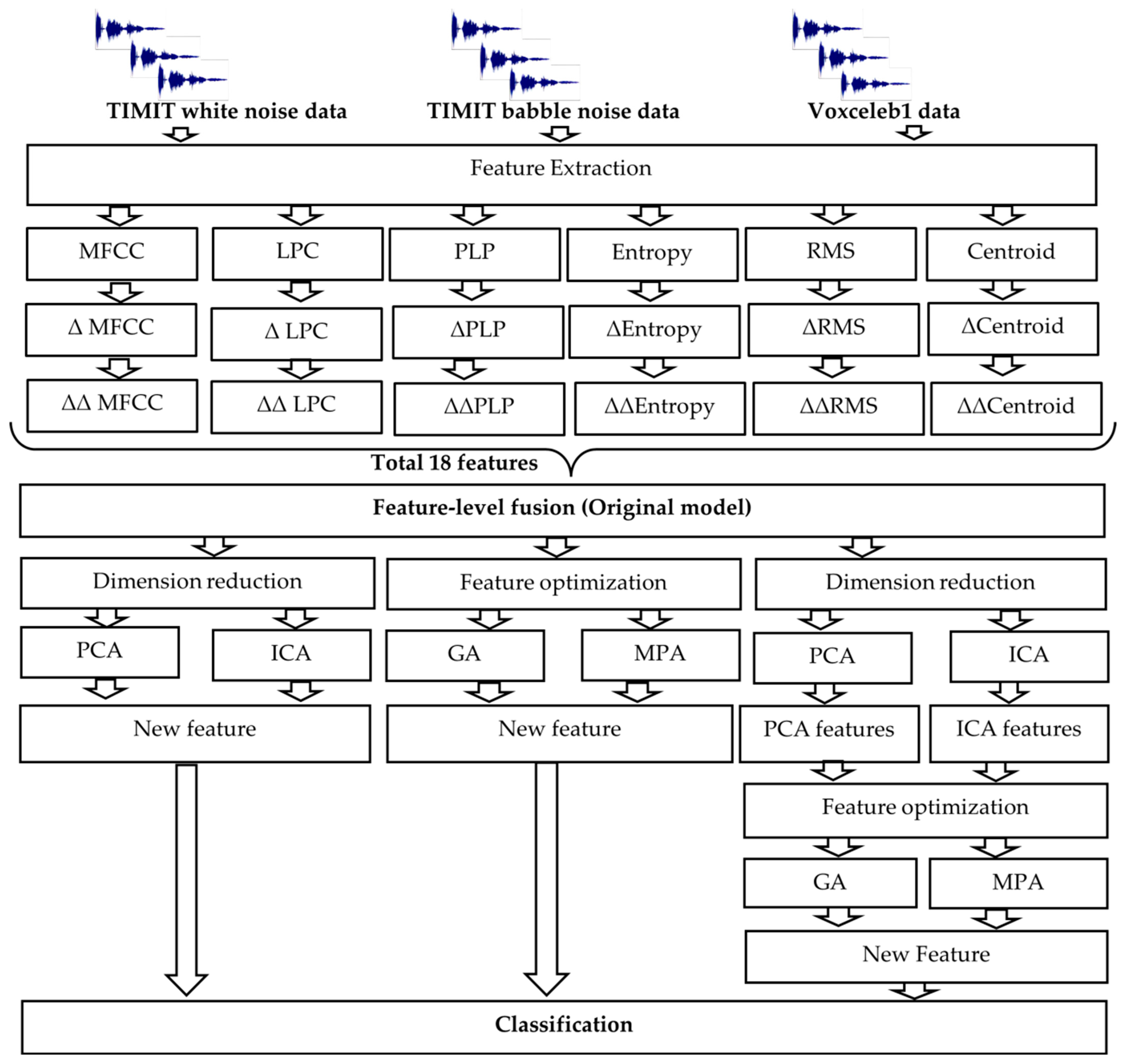
- Feature optimization using genetic algorithms (GAs) and the marine predator algorithm (MPA): While dimension reduction accelerates computation, it does not inherently identify the optimal feature set. To address this, we employ feature optimization methods like genetic algorithms (GAs) and the marine predator algorithm (MPA). Feature optimization is vital for enhancing machine learning model performance by selecting the most relevant features, reducing overfitting, improving computational efficiency, and promoting model interpretability. The proposed approach is illustrated in Figure 1, with comprehensive explanations provided in Section 3.2, Section 3.3 and Section 3.4.
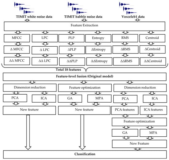 Figure 1. Proposed approach for the speaker recognition model.
3.2. The Feature Fusion Approach (Approach 1)
Feature fusion is a process that combines features derived from different sources or databases, creating a cohesive and enriched feature set. This integration enhances the distinctiveness of speech features, thereby facilitating more accurate classification and speaker identification [1]. While earlier studies have predominantly concentrated on features such as MFCC, LPC, and PLP [22,27,32], there exists a necessity to delve into additional acoustic features, as elaborated in Section 3.2.1. Figure 2 illustrates the feature fusion approach applied to voice data.
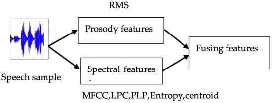
Figure 2.
The feature fusion approach.
3.2.1. Feature Extraction Techniques
The Mirtoolbox [51] is implemented in MATLAB (version 1.3.2, University of Jyväskylä, Finland) to compute the feature vectors. The following feature extraction methods are used in the proposed work.
The Mel-Frequency Cepstral Coefficient (MFCC)
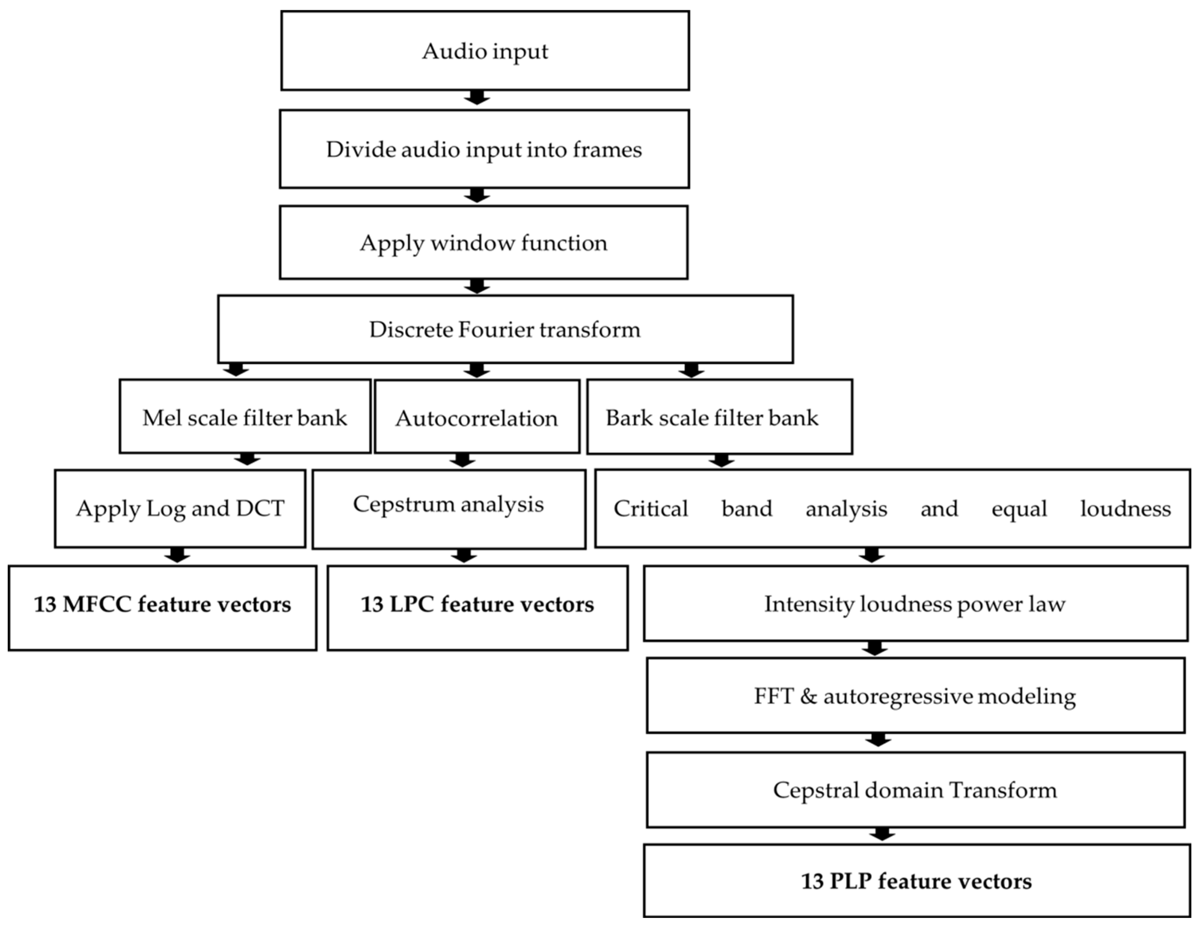
MFCCs, the predominant method for automatic speech recognition (ASR) feature extraction since the mid-1980s, involve a multistep process. This includes framing speech signals into segments lasting 20 to 40 milliseconds, applying windowing methods to account for the nonstationary nature of speech signals, transforming framed speech signals to the frequency domain using fast Fourier transform (FFT), passing the transformed signal through a mel filter bank based on the logarithmic mel scale, converting mel-scaled frequencies into a logarithmic scale, and applying discrete cosine transform (DCT) to select the primary 13 DCT coefficients as mel-frequency cepstral coefficient (MFCC) features, as established in [27,32,52,53,54] (Figure 3).
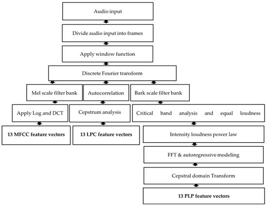
Figure 3.
MFCC, LPC and PLP feature extraction steps.
Linear Predictive Coding (LPC)
Linear predictive coding (LPC) is a method that computes the current sample by linearly combining past samples, and inverse filtering is utilized to eliminate formants from speech signals, resulting in a residual signal called the residue. The VQ-LBG algorithm is applied to calculate LPC features, where vector quantization (VQ) is implemented on LPC features in the linear spectral frequency (LSF) domain to reduce bitrate.
Understanding the autoregressive (AR) version of speech is crucial for LPC acquisition. The audio signal is modeled as a pth-order AR technique, represented by Equation (1), where each sample at the nth moment is influenced by ‘p’ preceding samples and gaussian noise u(n). LPC coefficients denoted by ‘a’ are obtained using Yule–Walker equations, as depicted in Equations (2)–(4), with the solution presented in Equation (5). For simplicity, only the first 13 LPC coefficients are employed. Further details on the proposed LPC features, the VQ-LBG algorithm, and calculation steps can be found in [55,56]. Linear predictive coding (LPC) is indeed a powerful technique, but it can have limitations, particularly concerning its sensitivity to variations in sample rate and its reliance on assumptions about speech signal properties. Therefore, in our proposed work, we complement LPC with a range of additional features to enhance the robustness and effectiveness of our speaker recognition system.
The final form of Yule–Walker equations is given by Equations (3) and (4).
Equation (7) gives the final solution to obtain LPC coefficients.
Perceptual Linear Prediction (PLP)
In this investigation, PLP features are selected due to their effectiveness in noise reduction, reverberation suppression, and echo elimination, contributing to overall improved performance. Previous research papers [27,52] have shown that combining PLP features with cepstral features results in enhanced outcomes in speaker recognition. The extraction of PLP features encompasses several steps, including equal loudness pre-emphasis, cube-root compression, and the elimination of irrelevant speech information. The comprehensive procedure for extracting PLP features is explained in references [22,57,58]. Thirteen PLP features are calculated by averaging all PLP features for each voice, effectively reducing system complexity using MATLAB software [57,58]. To align the dimensionality of PLP features with that of other features, the mean value of each frame is calculated, resulting in 13 × 1 feature vectors per frame. Figure 2 provides a visual representation of the feature extraction process for MFCC, LPC, and PLP features.
Spectral Centroid (SC)
The spectral centroid (SC) defines the center of gravity of the significance spectrum and is a unique value that represents the frequency area characteristic of a speech signal. A higher SC value corresponds to a higher signal strength [59]. It is calculated by Equation (6). The variable xi represents the ith frame of the speech signal, xi(k) refers to the amplitude value of the speech signal at the kth frequency bin within the ith frame.
Spectral Entropy (SE)
The following steps are used for the entropy feature calculation.
- For a signal x(t), calculate s(f), the power spectral density.
- Calculate the power within the spectral band based on the frequency of interest. Following the calculation of the spectral band power, normalize the power within the specified band of interest.
- Calculate the spectral entropy utilizing Equation (7) [60].
Root Mean Square (RMS)
The RMS is a measure of the loudness of a voice signal. It is calculated by taking the square root of the sum of the mean squares of the amplitudes of the sound samples. The RMS formula is given in Equation (8) [61], where x1, x2,…xn signify n observations, and xrms denotes the RMS value for the n observations.
Delta Features
Delta features are essential for capturing the rate of change in voice features, particularly the power dynamics of speech signals concerning noise. By incorporating delta (Δ) and delta–delta (ΔΔ) features, valuable dynamic information is extracted from speech signals [14,26,54]. The computation of the delta feature Δk involves subtracting the current feature fk from the previous feature fk−1, as represented in Equation (9).
Δk = fk − fk−1
Similarly, the delta–delta feature ΔΔk is obtained by subtracting the current delta feature Δk from the previous delta feature Δk−1, as depicted in Equation (10)
ΔΔk = Δk − Δk−1
Table 1 provides the dimensions of each feature utilized in this study.

Table 1.
Feature dimension.
3.2.2. Feature Fusion Methodology
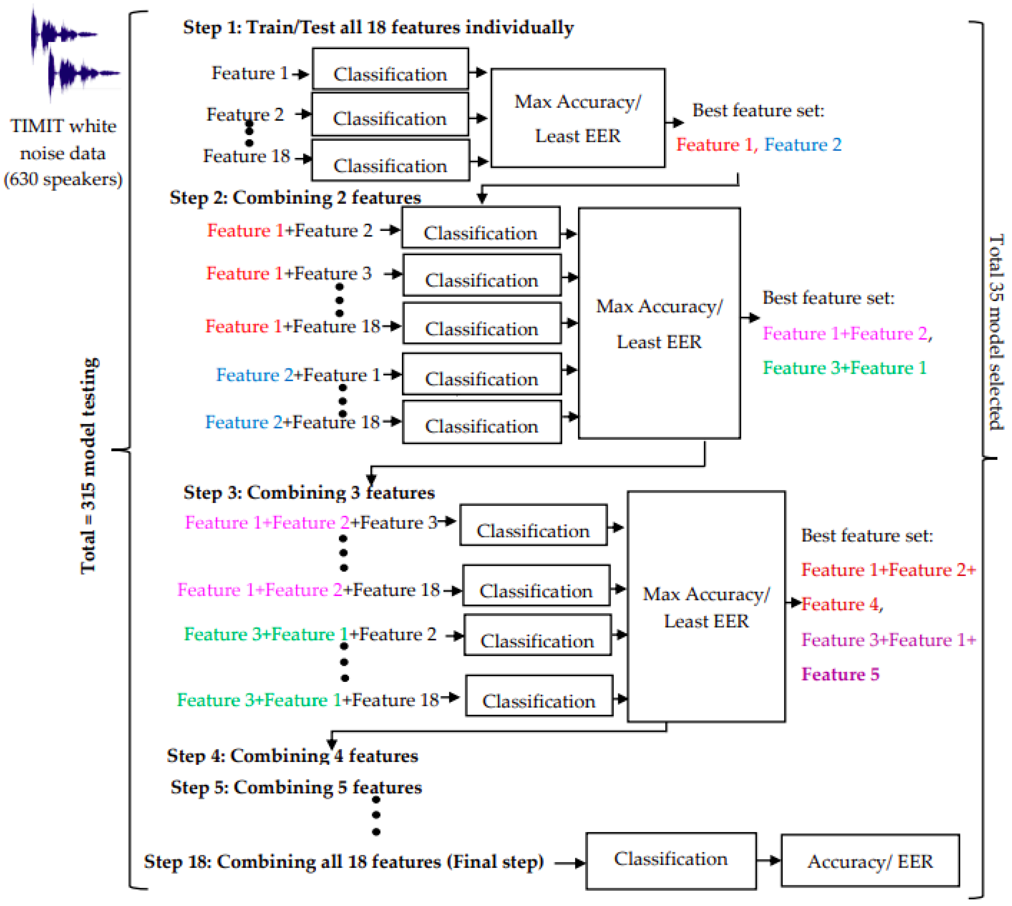
In this investigation, we followed the approach outlined in [1]. The following steps are used for the selection of the feature fusion model.
- All 18 features are tested individually for TIMIT white noise data with 630 speakers.
- Top 2 features with the highest SI accuracy and lowest average EER among the 18 features are selected.
- In determining the best model, the average accuracy and average EER values across three classifiers are considered. LPC and PLP emerge as the first and second-best features, respectively, with the highest average accuracies of 62.1% and 70.4%, surpassing other features. Equation (11) illustrates the calculation of average accuracy using the results from all three classifiers.
- 4.
- In the second stage, two features are fused by individually combining the best features LPC and PLP with the remaining 17 features. Once again, the top two models are selected from this process. The two best models identified in this step are the MFCC and LPC fusion model and the PLP and LPC fusion model.
- 5.
- In the third phase, three features are fused by individually combining the remaining 16 features with the two best models selected from step 2.
- 6.
- The fusion of features 4 to 18 is carried out in a similar manner, and the two best models are chosen at each step. In total, 315 models are tested for TIMIT white noise data. Figure 4 shows the workflow and methodology for feature aggregation using the TIMIT white noise 630 voice database.
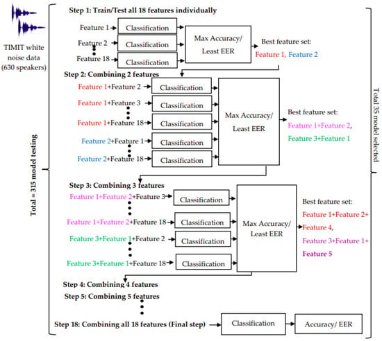 Figure 4. Flow diagram for best model selection approach using TIMIT white noise-630 speakers (approach 1).
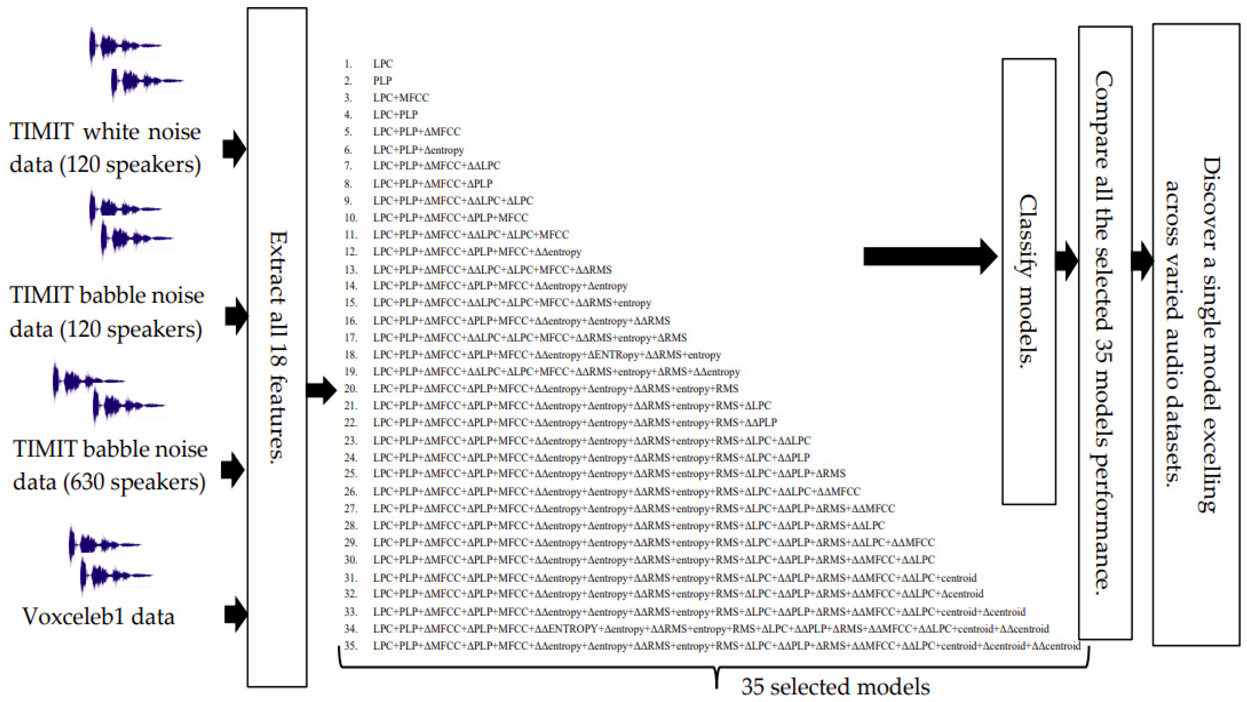
Out of 315 models, we identified the top 35 fusion models, which were exclusively employed for classifying the remaining datasets to expedite computation (see Figure 5). Repeating the training process for all 315 models across all datasets is exceedingly time-consuming.
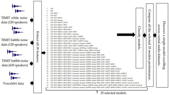
Figure 5.
Flowchart for model training with the top 35 models across different voice datasets.
Model Optimization
For computational efficiency, we have selected the top 35 models from Figure 4. These selected models will undergo testing on the remaining datasets.
Figure 5 outlines the workflow for training and testing the chosen 35 models. This process includes evaluating their performance on the following datasets:
- TIMIT white noise data with 120 speakers,
- TIMIT babble noise data with 120 speakers,
- TIMIT babble noise data with 630 speakers, and
- Voxceleb1 dataset.
This approach ensures thorough testing across various datasets while optimizing computational resources by focusing on the most promising models identified in the initial testing phase.
Figure 6 and Figure 7 explains the computation steps for speaker identification and speaker verification system, respectively.

Figure 6.
Speaker identification computation steps.

Figure 7.
Speaker verification computation steps.
3.3. Dimension Reduction Techniques (Approach 2)
Addressing the computational challenges associated with approach 1’s feature-level fusion, which demands substantial time and effort to identify the top models, a need for a more efficient solution arises. To overcome these challenges, dimension reduction algorithms have been developed, aiming to streamline computations by reducing the dimensionality of training data.
3.3.1. Principal Component Analysis (PCA)
One widely utilized technique in this context is principal component analysis (PCA). PCA addresses the curse of dimensionality by reducing the dimensionality of data while preserving most of its variance. In high-dimensional spaces, data points tend to be sparse, making it difficult to generalize and learn from them. PCA identifies the directions (principal components) along which the data varies the most and projects the data onto a lower-dimensional subspace spanned by these components. This reduces the dimensionality while retaining most of the important information in the data.
The steps involved in PCA are as follows [62]:
- Loading the input data: The feature fusion model, which serves as the input dataset, is loaded into the PCA algorithm.
- Subtracting the mean: The mean of the data is subtracted from each feature in the original dataset. This step ensures that the data are centered around the origin.
- Calculating the covariance matrix: The covariance matrix of the dataset is computed. This matrix captures the relationships and variations among the different features.
- Determining the eigenvectors: The eigenvectors associated with the largest eigenvalues of the covariance matrix are identified. These eigenvectors represent the directions of maximum variance in the dataset.
- Projecting the dataset: The original dataset is projected onto the eigenvectors obtained in the previous step. This projection transforms the data into a lower-dimensional subspace spanned by the eigenvectors.
- By following these steps, PCA effectively reduces the dimensionality of the dataset while preserving the most important information and capturing the most significant variations in the data [62,63].
3.3.2. Independent Component Analysis (ICA)
ICA was first introduced in the 1980s by J. Herault, C. Jutten and B. Ans, and the authors proposed an iterative real-time algorithm [64]. Independent component analysis (ICA) is a dimensionality reduction technique that aims to extract independent components from a dataset. It is an extension of PCA and provides a way to uncover hidden factors or sources that contribute to the observed data. ICA has gained significant attention in signal processing and data analysis due to its ability to separate mixed signals into their original sources.
The main steps involved in ICA can be summarized as follows:
- Preprocessing: Similar to PCA, the data are typically preprocessed by centroid and scaling the features to ensure a common reference point and equal contribution of each feature.
- Whitening: Whitening is performed to transform the data into a new representation where the features are uncorrelated and have unit variances. This step helps to remove any linear dependencies between the features.
- Defining the non-gaussianity measure: ICA aims to find components that are as statistically independent as possible. Different non-gaussianity measures can be used, such as kurtosis or negentropy, to quantify the departure from gaussianity and guide the separation of independent components.
- Optimization: The main objective of ICA is to maximize the non-gaussianity measure for each component. This is achieved through an optimization process, which involves finding the weights or mixing matrix that maximizes the non-gaussianity measure.
- Iterative estimation: ICA often involves an iterative estimation process to refine the separation of independent components.
- Reconstruction: Once the independent components are obtained, they can be used to reconstruct the original dataset or further analyzed for specific purposes such as feature extraction or signal separation [63,64,65,66].
For detailed steps on PCA, please refer to [62,63], and for ICA steps, [63,64,65,66]. These dimension reduction approaches contribute to a faster and more efficient identification of top models in the fusion process.
3.3.3. Model Optimization Using Dimension Reduction Techniques
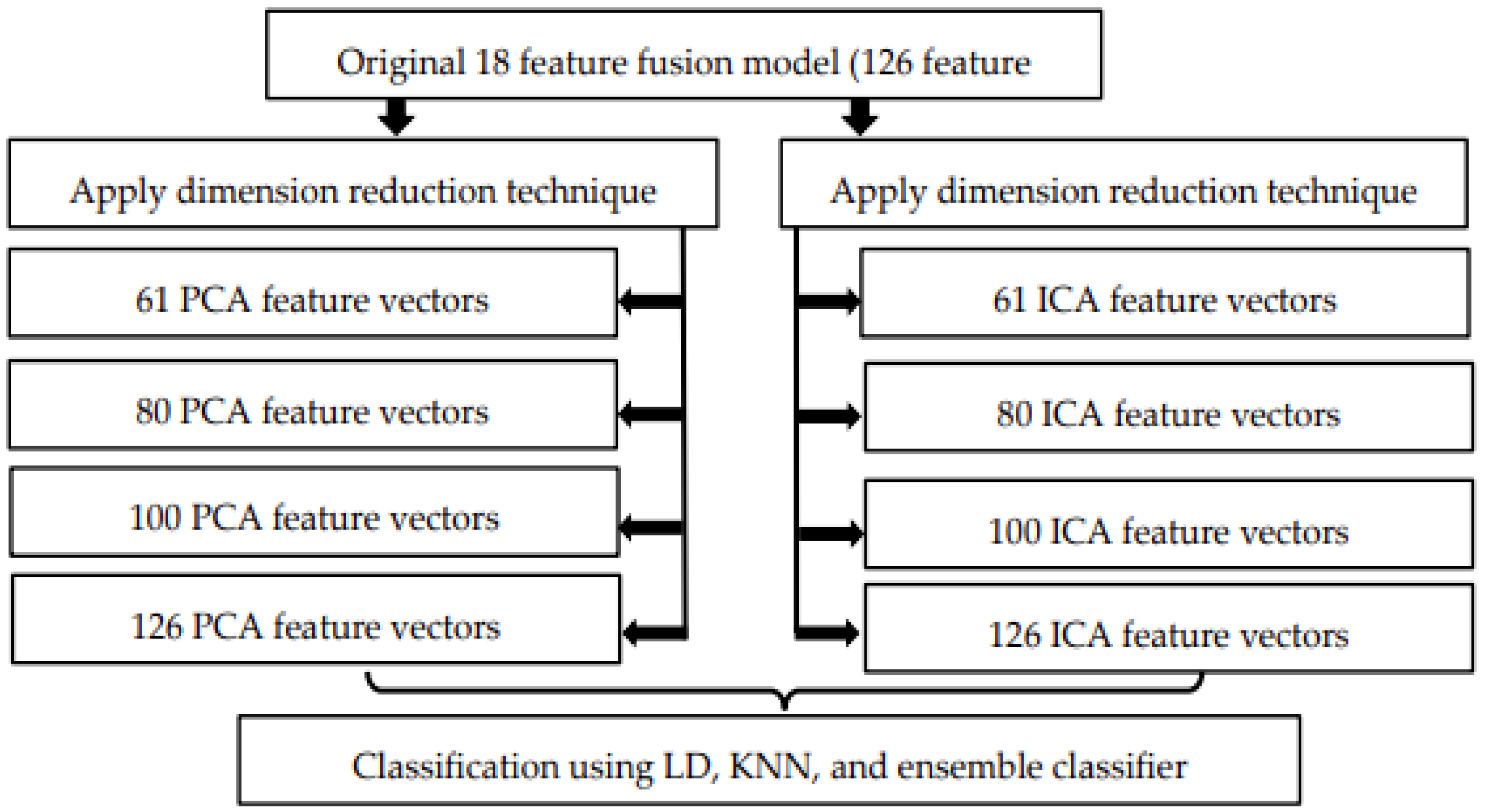
The following are the steps involved in model optimization using PCA and ICA. In our approach, we start by transforming the original model of 18 feature fusion having 126 feature vectors into 126 PCA and 126 ICA feature vectors.
- Then, we randomly reduced the feature vectors from 50% to 90% of their original size using PCA and ICA.
- Now, we have 3 new reduced PCA and ICA feature models and one 126 PCA and 126 ICA feature model.
- To evaluate the performance of the reduced dimension models, we employed LD, KNN, and ensemble classifiers.
- Accuracy, EER, and computation timing are calculated for each reduced model. Figure 8 explains the steps involved in model optimization using the dimension reduction technique for each dataset used.
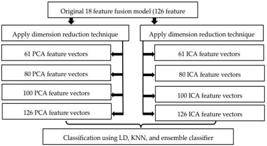 Figure 8. Model optimization using the dimension reduction technique (approach 2).
3.4. Feature Optimization (Approach 3)
While PCA and ICA are effective dimensionality reduction techniques, they do not inherently provide feature selection capabilities.
In contrast, feature selection approaches address this limitation by systematically evaluating the relevance and contribution of each feature in the dataset. By employing feature selection techniques, the effort and time needed for manual feature selection are reduced, as the algorithm automatically identifies the most informative features. This automated approach helps streamline the feature selection process and improves the efficiency of speaker recognition and other applications [1,2,3,4,5].
The proposed method uses wrapper-based feature selection with a KNN classifier. Wrapper-based feature selection offers optimality for specific algorithms, considers feature interactions, and provides flexible and adaptive selection, leading to more accurate and context-specific feature subsets. The referenced paper [67] may provide insights into accelerating this process using the K-nearest neighbor (KNN) algorithm, which can help reduce the computational burden while still leveraging the advantages of wrapper-based feature selection. In this proposed work, we use a genetic algorithm (GA) and the marine predator algorithm (MPA) feature selection method. The following sections explain the parameters and importance of the GA and MPA feature optimization methods.
3.4.1. Genetic Algorithms (GAs) [3,4]
Genetic algorithms (GAs) are optimization algorithms inspired by the process of natural selection and genetics. They are used to find solutions to optimization and search problems.
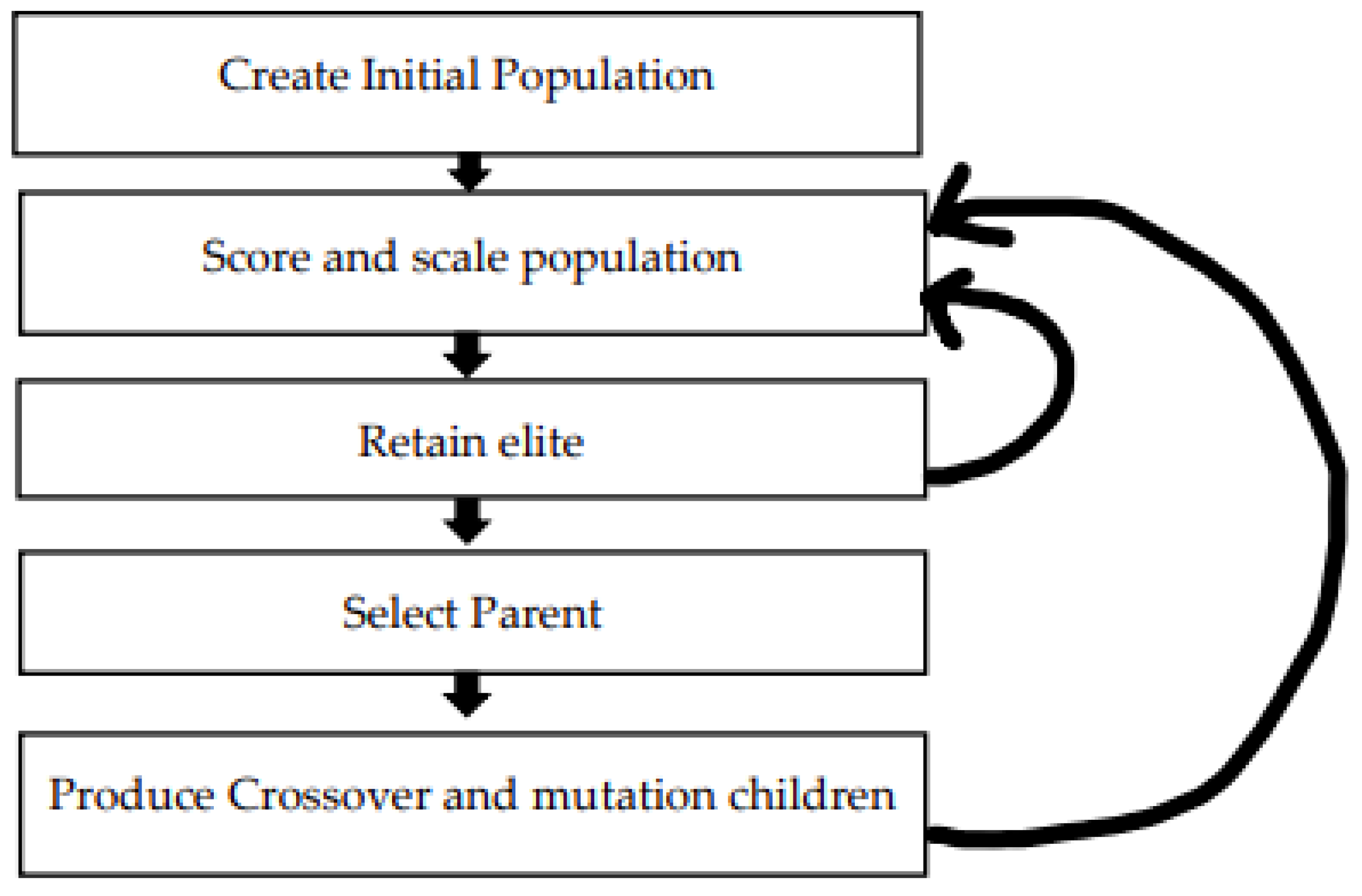
Their robustness and adaptability make them valuable tools for identifying optimal feature subsets that enhance speaker recognition system performance [3,4]. Following are the computation steps for a genetic algorithm (GA) (Figure 9).
- Initialization: Generate an initial population of solutions.
- Evaluation: Assess each solution’s fitness using a defined function.
- Selection: Choose individuals from the population based on their fitness.
- Crossover: Combine selected individuals to create offspring.
- Mutation: Introduce random changes to offspring.
- Replacement: Create the next generation by combining parents and offspring.
- Termination: Stop the algorithm when a termination condition is met.
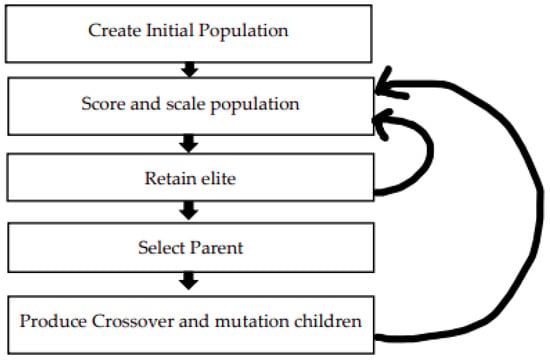
Figure 9.
Computation steps for GA.
Figure 9.
Computation steps for GA.
3.4.2. The Marine Predator Algorithm (MPA) [5,6]
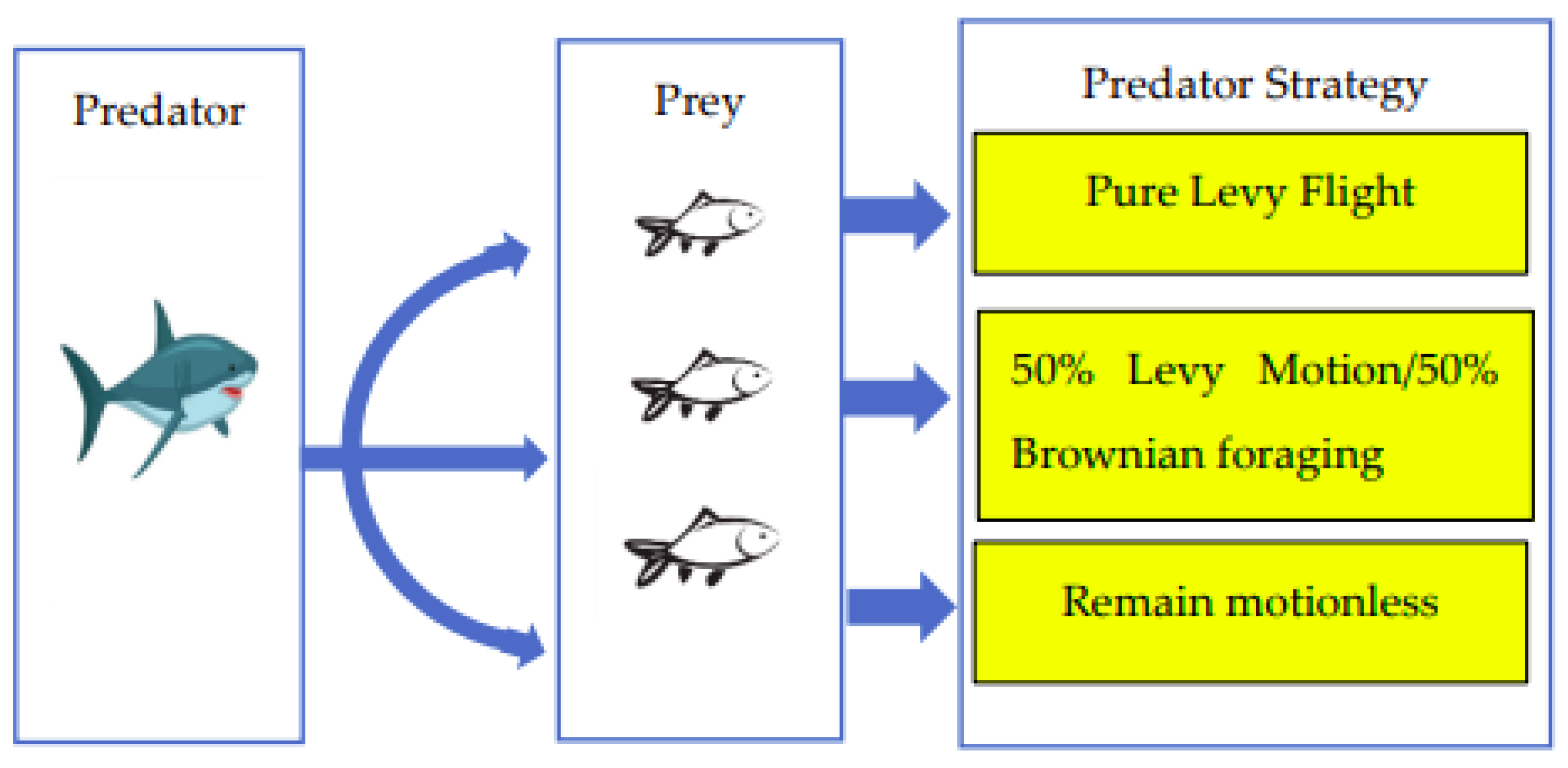
The marine predator algorithm (MPA) is a nature-inspired optimization algorithm that simulates the hunting behavior of marine predators in finding their prey.
The optimization process in MPA comprises three distinct phases, illustrated in the figure. These phases are categorized based on the velocity ratio and time.
- Phase 1: The predator moves at a slower pace than the prey, characterized by a high velocity ratio.
- Phase 2: The predator and prey maintain nearly identical speeds, representing a unity velocity ratio.
- Phase 3: The predator accelerates and moves faster than the prey, indicating a low velocity ratio.
Here are the typical steps involved in the marine predator algorithm:
- Initialization: Start with a population of marine predators.
- Prey Location: Determine the location of potential prey.
- Predation: Update predator positions towards the prey.
- Encounter: Check if predators have caught the prey.
- Feeding: If caught, adjust predator positions accordingly.
- Behavior Update: Modify predator behavior based on success.
- Termination: Decide when to stop the algorithm.
- Iteration: Repeat steps 2–7 until termination criteria are met.
The complete steps and implementation details of the MPA with a KNN classifier using the provided parameters can be found in referenced papers [5,6]. Figure 10 shows important strategy for the marine predator algorithm.
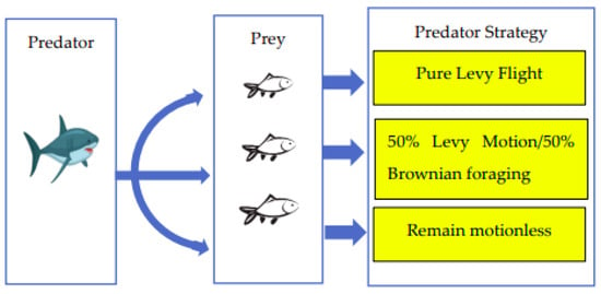
Figure 10.
MPA strategy for feature optimization.
3.4.3. Model Optimization Using the Feature Selection Approach
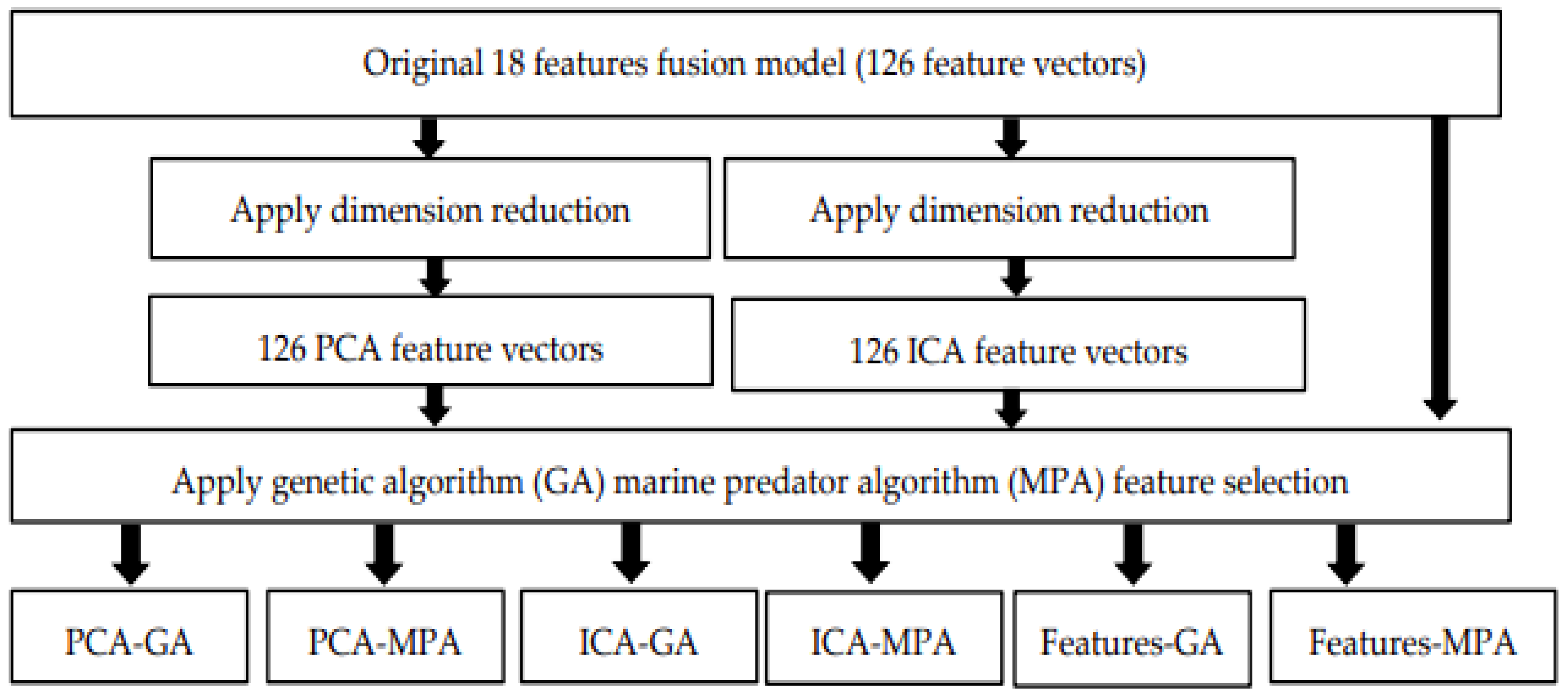
The feature selection process involved considering three sets of feature vectors: original, PCA, and ICA. Subsequently, feature optimization was applied to these three models, resulting in six new reduced feature models: PCA-GA, PCA-MPA, ICA-GA, ICA-MPA, Features-GA, and Features-MPA (as shown in Figure 11). The performance of these six new reduced feature sets, along with the original feature set, was then assessed to identify the best-performing model among them. Figure 11 illustrates the proposed feature optimization steps.
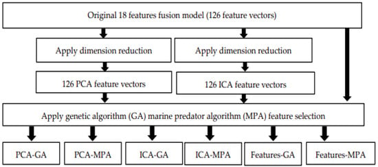
Figure 11.
Model optimization using feature selection methods.
3.5. Classification
All classification tasks are performed using the classification learner application in MATLAB. The following classifiers are used in the proposed work.
3.5.1. Linear Discriminant (LD) Classifier
The LD classifier uses Bayes’ theorem to compute probabilities. The output class is denoted as k and the input is denoted as x; then, Bayes’ theorem is employed to determine the probability that the data belong to each class, as shown in Equations (12) and (13).
In the above equation, PIk is the prior probability, which is the base probability of each class, as observed in the training data.
- The function f(x) is an expected probability that x belongs to a particular class and employs a gaussian distribution function. Here, n denotes the number of instances, and K is the number of classes.
- By combining the gaussian distribution into the equation and simplifying, we obtain Equation (14). This function serves as a discriminant, and the class with the highest calculated value is the output classification (y).
- Dk(x) represents the discriminant function for class k given input x, where (mean vector), σ2, and PIk are all calculated from the data [68]. Figure 12 shows data points using a LD classifier.
 Figure 12. Linear discriminant classification.
3.5.2. K Nearest Neighbor Classification (KNN)
The K-nearest neighbors (KNN) approach is a classification method employed to categorize unknown data points based on their resemblance to neighboring data points (Figure 13). In this approach, the parameter K indicates the number of dataset elements contributing to the classification process, and for this specific work, K is set to 1. The KNN algorithm can be summarized in the following steps [69].
- Choose a value for K, which represents the number of neighbors.
- Compute the Euclidean distance between the unknown data point and its K nearest neighbors.
- Classify the K nearest neighbors based on the computed Euclidean distances.
- Count the number of data points in each class.
- Assign the new data point to the class with the highest count.

Figure 13.
KNN classification.
Figure 13.
KNN classification.

3.5.3. Ensemble Classification
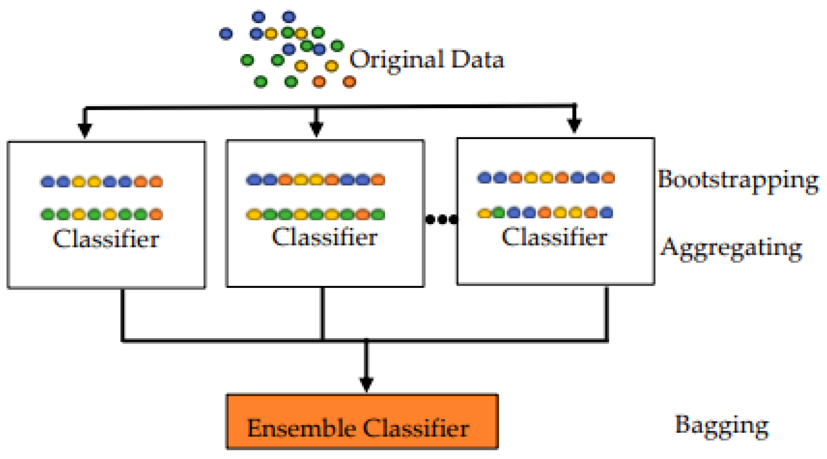
In this study, an ensemble classification method is employed to improve the speaker recognition results and address overfitting [70]. The proposed ensemble classifier utilizes the random subspace ensemble method, consisting of 30 learners with a subspace dimension of 5. Following steps are involved for ensemble classification (Figure 14).
- Bootstrap sampling: Create multiple bootstrap samples by randomly sampling with replacement from the original dataset.
- Base learner training: Train a base classifier decision tree on each bootstrap sample independently.
- Voting or averaging: Combine predictions of all base classifiers using majority voting.
- Reduced variance: By aggregating predictions from diverse models trained on different subsets of the data, bagging reduces variance and improves generalization performance [70,71].
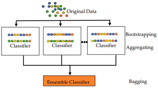
Figure 14.
Ensemble classification.
Figure 14.
Ensemble classification.
4. Evaluation
4.1. Database Preparation
The following three voice databases are used in the proposed work, and their explanations are as follows.
- In this research work, we incorporated the noisy TIMIT speech dataset developed by the Florida Institute of Technology, which consists of approximately 322 h of speech from the TIMIT acoustic-phonetic continuous speech corpus (LDC93S1). The dataset was modified by adding different levels of additive noise while keeping the original TIMIT arrangement intact. For our study, we specifically focused on TIMIT white noise and babble noise with a 30 dB noise level. We selected subsets of the dataset containing 120 speakers for TIMIT babble and white noise and 630 speakers for TIMIT white and babble noise. Each speaker contributed a total of 10 utterances. For TIMIT babble and white noise with 120 speakers, we used 720 voice samples for training and 480 voice samples for testing, resulting in a total of 1200 voices.
- Similarly, for TIMIT babble and white noise with 630 speakers, we used 5040 voice samples for training and 1260 voice samples for testing, totaling 6300 voices [72]. This approach allowed us to make fair comparisons with other studies, including [41,42]. In the context of the TIMIT dataset or any similar speech dataset, when referring to a specific SNR level such as “30 dB”, it typically represents the ratio of the signal power to the noise power on average. Therefore, it refers more to the mean noise level rather than the peak noise level.
- The voxceleb1 dataset is known for its large size, as it contains over 100,000 voice samples. The videos in this database were recorded in diverse and challenging multispeaker environments, such as outdoor stadiums, where real-world noise, such as laughter, overlapping speech, and room acoustics, is introduced to degrade the datasets. For our research paper, we utilized data from 1251 speakers and a total of 153,516 speaker voices. To ensure a fair comparison with [47,48], we carefully selected 148,642 utterances for training and 4874 utterances for testing in the context of speaker verification tasks. For speaker identification, we utilized 145,265 utterances for training and 8251 utterances for testing.
- TIMIT and voxceleb1 voice datasets consist of full English sentences, making it suitable for analyzing speech at the sentence level. The dataset details, along with the number of utterances used for training and testing, are shown in Table 2 for reference.
 Table 2. Database details.
 - We divided our data using the same method as utilized by other researchers to ensure a fair comparison. Specifically, for the TIMIT dataset, we followed the data split used by [46] for 630 speakers and [42,43] for 120 speakers. Similarly, for the VoxCeleb1 dataset, we employed the same data split as described in [47,48,49,50] to ensure consistency and fairness in our comparisons. This approach allowed us to conduct meaningful evaluations while maintaining parity with existing studies.
4.2. Assessing the Effectiveness of Speaker Identification (SI)
Speaker identification accuracy assesses a system’s ability to correctly recognize different speakers based on their voice. It holds significance as it guarantees security, personalization, efficiency, and convenience across applications utilizing voice-based interaction or authentication. The SI accuracy, computed using MATLAB’s classification learner application, encompasses all proposed models with all three classifiers. Simplified result tables display only the models with the highest accuracy. Accuracy is determined by the number of correctly identified speaker voices divided by the total number of voices in the dataset (Equation (15)).
4.3. Assessing the Effectiveness of Speaker Verification (SV)
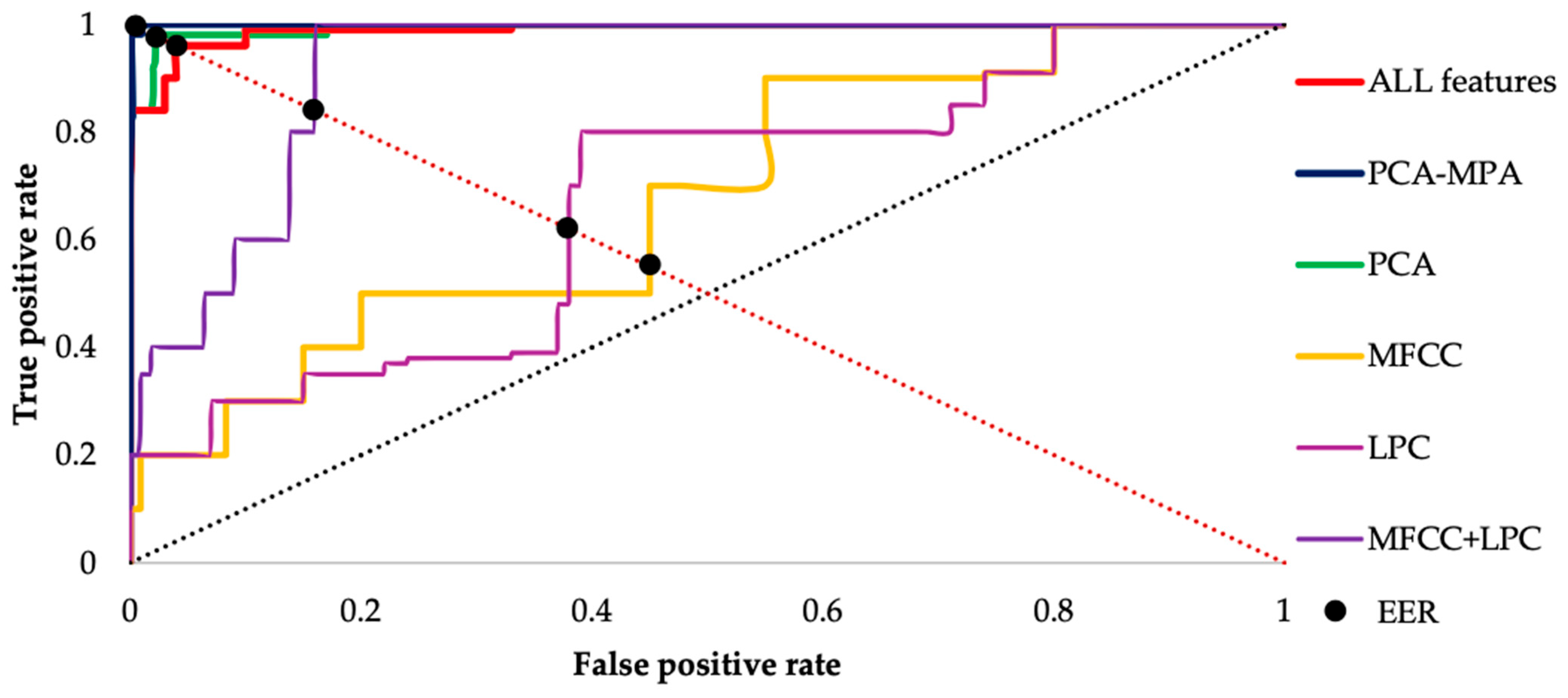
For the SV task, EER values are computed using MATLAB for each model. EER is determined from the point of intersection between the receiver operating characteristic (ROC) curve and the diagonal axis running from (0, 1) to (1, 0), which corresponds to the false positive rate [73,74]. To conduct a more comprehensive comparison between the proposed method and existing methods, we assess the EER values of the top-performing models.
Figure 15 depicts the ROC curve and EER point using a KNN classifier for single MFCC features (yellow line), LPC features (blue line), fusion of MFCC and LPC features (purple line), all 18 features (red line), dimension reduction method PCA (green line) and feature optimization method PCA-MPA (indigo line), We observe that the ROC curve closer to (1, 0) yields the lowest EER, hence indicating better performance compared to other methods used. Therefore, based on this curve, we can say that the feature optimization method is providing the best results among all the methods employed.
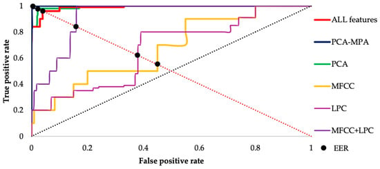
Figure 15.
Receiver operating characteristic curve (ROC) for voxceleb1 data with a KNN classifier.
5. Results Discussion
The result table simplifies by including only the top results.
5.1. Optimal Outcomes Utilizing Feature-Level Fusion (Approach 1)
Table 3, Table 4, Table 5, Table 6 and Table 7 displays the outcomes of speaker recognition using individual features such as MFCC and LPC, as well as their fusion, alongside the performance metrics of the top-performing feature fusion model. This model achieves the highest accuracy and lowest equal error rate (EER) across experiments conducted on TIMIT babble noise (120,630 speakers), TIMIT white noise (120,630 speakers), and voxceleb1 data. The data presented highlight the superiority of combining multiple features, consistently outperforming the use of single features or fewer combinations. Only the classification method delivering the best results is included in Table 3, Table 4, Table 5, Table 6 and Table 7.

Table 3.
Result comparison table using the feature-level fusion approach for TIMIT babble noise data (120 speakers).

Table 4.
Result comparison table using the feature-level fusion approach for TIMIT babble noise data (630 speakers).

Table 5.
Result comparison table using the feature-level fusion approach for TIMIT white noise data (120 speakers).

Table 6.
Result comparison table using the feature-level fusion approach for TIMIT white noise data (630 speakers).

Table 7.
Result comparison table using the feature-level fusion approach for voxceleb1 data.
For the TIMIT babble noise database, the best SI accuracy and EER values achieved using the linear discriminant (LD) classifier are 92.7% (120 speakers) and 89.3% (630 speakers), with EER values of 4.4% and 2.2%, respectively. The models with the fusion of 12 features and 14 features obtain the best results for the 120 and 630 speaker datasets, respectively (Table 3 and Table 4).
Similarly, for the TIMIT white noise database, the best SI accuracy and EER values using the LD classifier are 93.3% (120 speakers) and 79.4% (630 speakers), with EER values of 1.1% and 2.4%, respectively. The models with the fusion of 11 features and 12 features obtain the best results for 120 and 630 speakers, respectively (Table 5 and Table 6).
For the voxceleb1 database, the highest SI accuracy achieved is 90%, and the lowest EER of 4.07% [1] is achieved using the fusion of 14 features with the KNN classifier in Table 7. Table 3, Table 4, Table 5, Table 6 and Table 7 clearly demonstrates the enhancement in speaker recognition results when employing feature combinations rather than single features.
Table 8, Table 9 and Table 10 demonstrate the varied performance of different classification methods when combining all 18 features for various numbers of speakers. In the case of TIMIT data with 120 speakers (considered small data) and 630 speakers (considered medium data), the linear discriminant classifier (LD) exhibited superior speaker identification accuracy, achieving 89.8% and 86.9% for babble and white noise, respectively, with 120 speakers, and 89.9% and 79.2% for white noise with 630 speakers. However, when considering equal error rate (EER), the K-nearest neighbors (KNN) classifier yielded better results overall, with 0.77% and 1.1% for babble noise with 120 and 630 speakers, respectively, and 1.2% and 0.16% for white noise data for120 and 630 speakers, respectively. It can be concluded that both linear discriminant and KNN classifiers are suitable for small and medium-sized datasets. Conversely, in the case of the large voxceleb1 dataset as shown in Table 6, the KNN classifier outperformed others, achieving 89.7% accuracy with a 4.5% error rate. Additionally, KNN demonstrated comparatively faster computation times compared to other classifiers utilized in this study.

Table 8.
SI accuracy and EER using all feature models for all databases with babble noise (126 features).

Table 9.
SI accuracy and EER using all feature models for all databases with white noise (126 feature vectors).

Table 10.
SI accuracy and EER using all feature models for all databases with voxceleb1 noise (126 feature vectors).
Figure 16, Figure 17, Figure 18, Figure 19 and Figure 20 depict the fluctuation in speaker identification accuracy with varying numbers of feature fusion across different classification methods for babble noise (120 speakers and 630 speakers), white noise (120 speakers and 630 speakers), and voxceleb1 data, respectively. Analysis of the graphs reveals that increasing the number of features generally enhances accuracy. However, it is notable that indiscriminate addition of features does not guarantee improved results. Also, different combinations of feature perform differently with different classifiers. To address this variability and ensure optimal performance, we propose feature optimization techniques. These techniques aim to identify the most informative features while minimizing redundancy, thereby maximizing the discriminative power of the feature set. By employing feature optimization, we can streamline the feature fusion process, enhancing the robustness and effectiveness of speaker identification systems across diverse noise conditions and dataset sizes.

Figure 16.
Change in SI accuracy using various numbers of features combination for babble noise 120 speakers.

Figure 17.
Change in SI accuracy using various numbers of features combination for babble noise 630 speakers.

Figure 18.
Change in SI accuracy using various numbers of features combination for white noise 120 speakers.

Figure 19.
Change in SI accuracy using various numbers of features combination for white noise 630 speakers.

Figure 20.
Change in SI accuracy using various numbers of features combination for voxceleb1 data.
5.2. Optimal Outcomes Utilizing the Dimension Reduction Technique (Approach 2)
Table 11 displays the best results achieved using PCA for dimension reduction and includes the computational times for training and testing. Since PCA outperforms ICA, only the PCA results are shown. Figure 21, Figure 22 and Figure 23 shows the comparison of a PCA and ICA dimension reduction technique with various datasets used.

Table 11.
Best model using dimension reduction (approach 2).
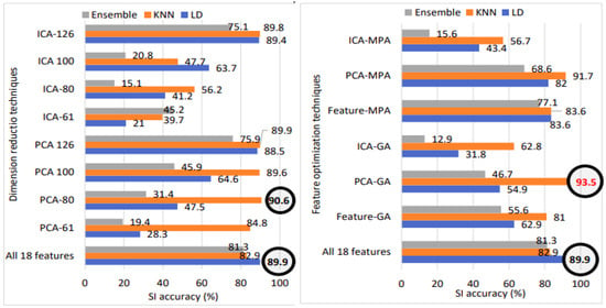
Figure 21.
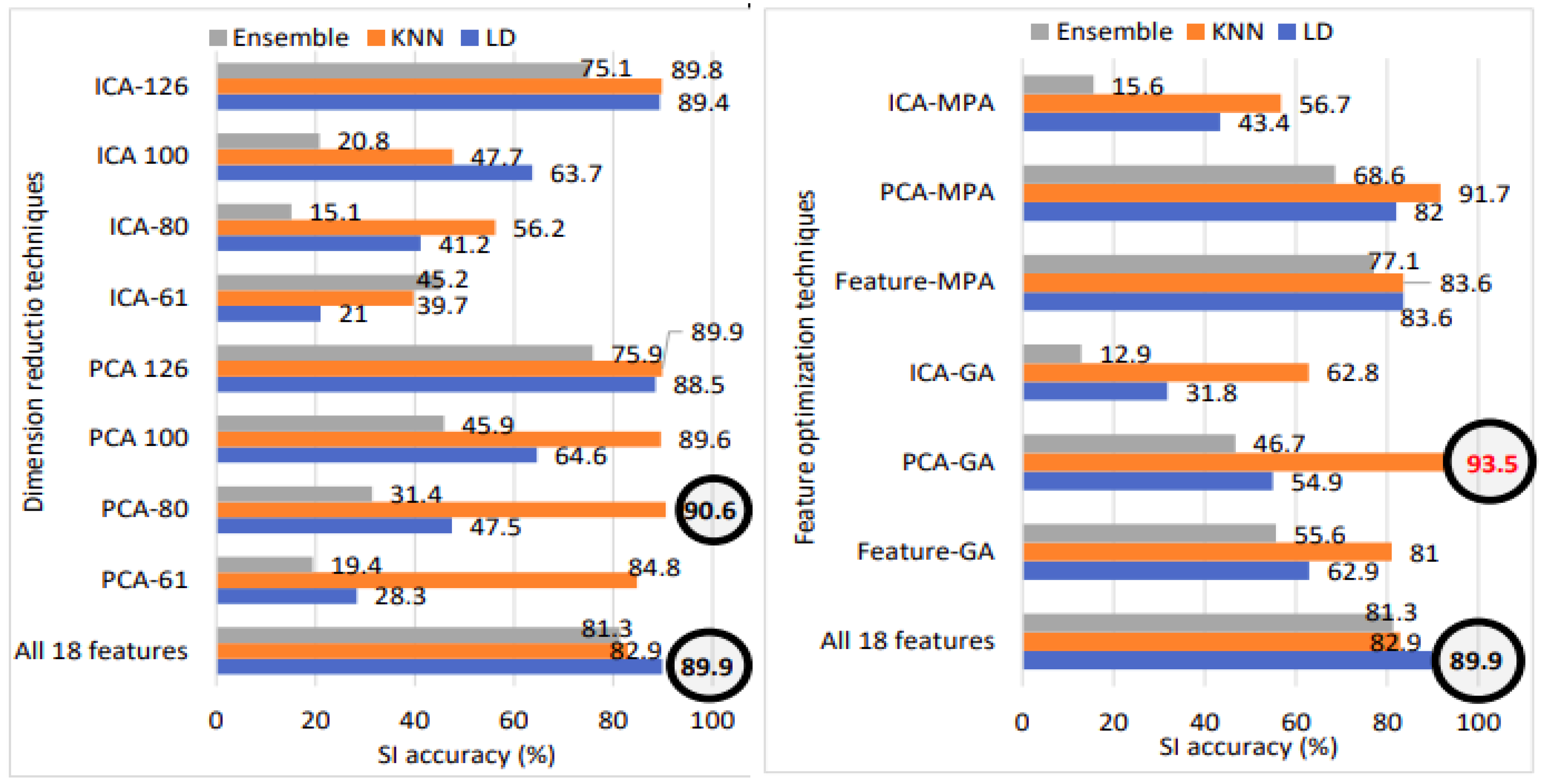
SI accuracy with various methods on TIMIT babble noise dataset: All 18 features, fusion, dimension reduction, and feature optimization.
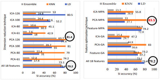
Figure 22.
SI accuracy with various methods on TIMIT white noise dataset: All 18 features, fusion, dimension reduction, and feature optimization.

Figure 23.
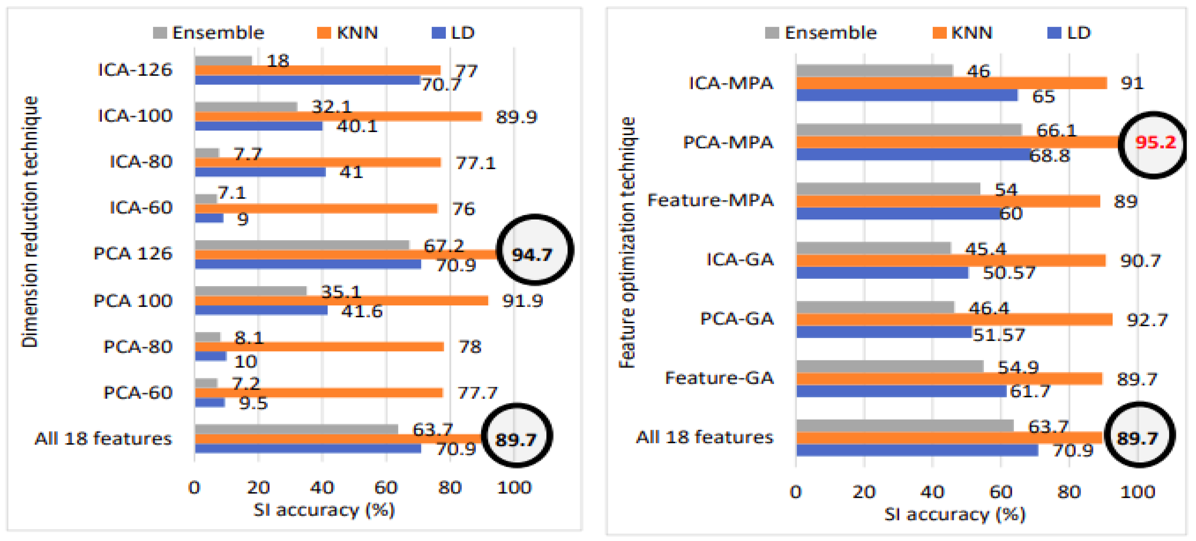
SI accuracy with various methods on voxceleb1 dataset: All 18 features, fusion, dimension reduction, and feature optimization.
From Table 11, we can observe that the TIMIT babble noise database with 120 speakers, the best SI accuracy of 89.9% and an EER of 0.9% are achieved using 126 PCA feature vectors with the LD classification method. For TIMIT babble noise with 630 speakers, the best SI accuracy of 90.6% and an EER of 0.69% are achieved using 80 PCA feature vectors with the KNN classifier.
In the case of TIMIT white noise data with 120 speakers, the best SI accuracy of 93.3% and an EER of 0.58% are achieved using 100 PCA feature vectors with the KNN classification. For TIMIT white noise with 630 speakers, the best SI accuracy of 81.4% and an EER of 0.13% are achieved using 126 PCA feature vectors with the KNN classification.
For the voxceleb1 database, the best SI accuracy of 94.7% and the lowest EER of 2.2% are achieved using 126 feature vectors with the KNN classifier. For voxceleb1 data, we can observe that performance improves using dimension reduction techniques compared to approach 1 [1]. For the TIMIT babble noise data with 120 speakers, the linear discriminant classifier with PCA 126 feature vector gives a high accuracy of 89.9% and lowest EER of 0.9%; for the other dataset, KNN performs better with various numbers of PCA vectors.
5.3. Optimal Results Achieved with the Feature Optimization Technique (Approach 3)
Table 12 presents the most promising outcomes attained through feature optimization using the proposed methods.

Table 12.
Best model using feature optimization (approach 3).
For babble noise data with 120 and 630 speakers, the best accuracy achieved was 85.6% and 93.5%, with EER values of 0.7% and 0.13%, respectively, using the KNN classification. The feature vectors were reduced to 81 for the TIMIT babble noise 120 speakers and 90 for the TIMIT babble noise 630 speakers using the PCA-GA approach 3. Regarding the TIMIT white noise data, the best accuracies achieved were 87.9% and 83.5% for 120 and 630 speakers, respectively, with the best EER values of 0.8% and 0.13%, respectively. The optimal performance was achieved using the PCA-MPA feature optimization method with the KNN classifier, with reduced feature vectors of 103 and 112 on the 120 and 630 speaker TIMIT white noise data, respectively.
For the voxceleb1 data, the PCA-MPA feature optimization method with 112 reduced feature vectors and the KNN classifier achieved the best accuracy of 95.2% and an EER of 1.8%. The results indicate that PCA-based optimization approaches, namely, PCA-GA and PCA-MPA, demonstrate superior performance in comparison to other methods.
5.4. A Performance Comparison across Feature-Level Fusion, Dimension Reduction, and Feature Optimization Indicates their Overall Effectiveness
Figure 21 illustrates the speaker identification performance comparison among all 18 features, dimension reduction, and feature optimization for babble noise data with 630 speakers. Notably, utilizing all 18 features results in an SI accuracy of 89.9%. Transitioning to PCA with 80 feature vectors boosts accuracy to 90.6%. However, applying genetic algorithm feature optimization to the original PCA vectors elevates accuracy to an impressive 93.5%. Hence, the application of GA on PCA feature vectors emerges as the overall best-performing model, represented in bold red font.
Figure 22 illustrates the speaker identification performance comparison among all 18 features, dimension reduction, and feature optimization for white noise data with 630 speakers. Notably, utilizing all 18 features results in an SI accuracy of 79.2%. Transitioning to PCA with 126 feature vectors boosts accuracy to 81.4%. However, applying marine predator algorithm (MPA) feature optimization to the original PCA vectors elevates accuracy to an impressive 83.5%. Hence, the application of MPA on PCA feature vectors emerges as the overall best-performing model, represented in bold red font.
Figure 23 illustrates the speaker identification performance comparison among all 18 features, dimension reduction, and feature optimization for voxceleb1 data. Notably, utilizing all 18 features results in an speaker identification accuracy of 89.7%. Transitioning to PCA with 126 feature vectors boosts accuracy to 94.7%. However, applying marine predator algorithm (MPA) feature optimization to the original PCA vectors elevates accuracy to an impressive 95.2%. Hence, the application of MPA on PCA feature vectors emerges as the overall best-performing model, represented in bold red font.
5.5. Comparative Analysis of Computational Timing: Feature-Level Fusion, Dimension Reduction, and Feature Optimization Techniques
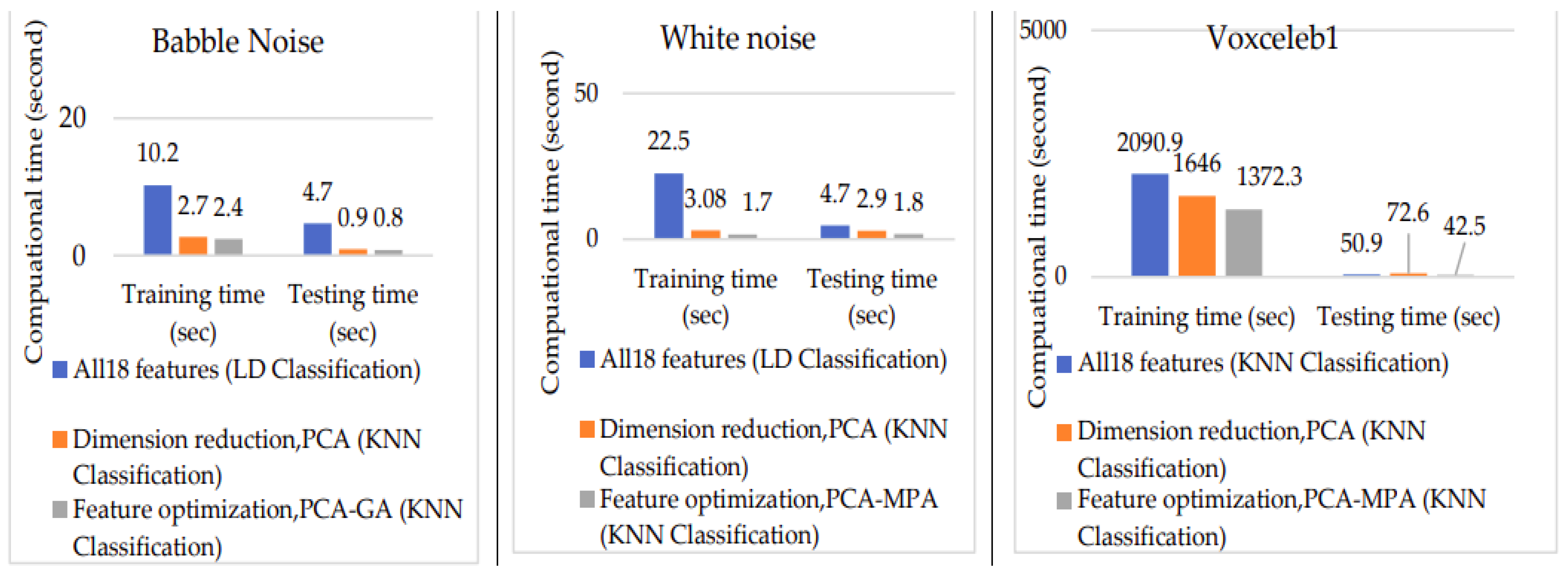
Figure 24 presents the computation time comparison between using all 18 features and the best model achieved through dimension reduction and feature optimization. Notably, computation time decreases with dimension reduction and feature optimization compared to feature fusion.
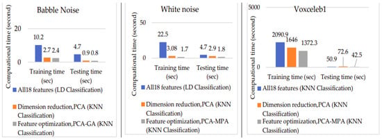
Figure 24.
Computation time comparison graph.
For TIMIT babble noise data, training and testing time using all 18 features are 10.2 s and 4.7 s, respectively. With PCA dimension reduction, training time reduces to 2.7 s, and testing time decreases to 0.9 s. Further improvement is observed with PCA-GA feature optimization, achieving training and testing times of 2.4 s and 0.8 s, respectively.
Similarly, for TIMIT white noise data, training and testing time using all 18 features are 22.5 s and 4.7 s, respectively. Utilizing PCA dimension reduction results in a training time of 3.08 s and a testing time of 2.9 s. PCA-MPA feature optimization further enhances efficiency, achieving training and testing times of 1.7 s and 1.8 s.
For voxceleb1 data, training and testing time using all 18 features are 2090.9 s and 50.9 s, respectively. PCA dimension reduction reduces training time to 1646 s and testing time to 72.6 s. PCA-MPA feature optimization demonstrates even greater efficiency, with training and testing times of 1372.3 s and 42.5 s. Figure 24 illustrates that feature optimization is notably faster compared to other approaches.
5.6. Comparing the Proposed Work with the Existing Approach
Table 13, Table 14 and Table 15 present the best results achieved by the three proposed approaches on all datasets, and we compare these results with other best results obtained using the same input data for each dataset. Limited research has been conducted using the 30 dB TIMIT noisy dataset. To address this gap, we included reference [46], which utilized the same number of speakers but with babble and white noise. Additionally, we ensured fairness by testing our system on 120 speakers from the TIMIT dataset, following the same training and testing protocols outlined in [42,43]. This approach allowed for a rigorous and unbiased comparison of results.

Table 13.
Result comparison for TIMIT babble noise.

Table 14.
Result comparison for TIMIT white noise.

Table 15.
Result comparison for voxceleb1.
5.6.1. Result Comparison for TIMIT Babble Noise (120 Speakers)
The highest speaker identification accuracy of 92.7% is achieved using feature-level fusion (approach 1) with 12 features and LD classification (Table 13). The lowest EER of 0.13% is achieved using PCA-GA feature selection (approach 3) (Table 13). In comparison, The studies in [45,46] achieved the best EER values of 4.3% and 6.39% using GMM and i-vector approaches with 368 and 630 speakers, respectively, for babble noise data.
5.6.2. Result Comparison for TIMIT Babble Noise (630 Speakers)
The best speaker identification accuracy and EER of 93.5% and 0.13% are achieved using PCA-GA feature selection with the KNN classifier (Table 13). In comparison, the studies in [45,46] achieved EER values of 4.3% and 6.39% using GMM and i-vector approaches for babble noise data.
5.6.3. Result Comparison for TIMIT White Noise (120 Speakers)
For a fair comparison of results, we conducted tests on 120 speakers, using the same training and testing methodologies as described in [42,43]. Notably, our model achieved the highest speaker identification (SI) accuracy of 93.3% and the lowest equal error rate (EER) of 0.58% when employing PCA dimension reduction (approach 2) with 100 feature vectors (refer to Table 14).
In contrast, previous studies [42,43] reported lower accuracies, with the highest SI accuracies of 75.83% and 79.17%, respectively, using score-level fusion techniques on the same dataset comprising 120 speakers and 30-dB noisy data. Remarkably, our PCA-based dimension reduction method outperformed [42,43] in terms of accuracy.
Furthermore, even when scaling up to a dataset of 630 speakers, our model consistently demonstrated superior accuracy compared to the existing research reported in [42,43].
5.6.4. Result Comparison for TIMIT White Noise (630 Speakers)
The highest SI accuracy of 83.5% and lowest EER of 0.13% are achieved using PCA-MPA feature optimization (approach 3) with 112 selected feature vectors and the KNN classifier (Table 14). In comparison, refs. [44,45], and [46] achieved accuracies of 63% and EER values of 7.1% and 8%, respectively, using GMM and i-vector approaches.
5.6.5. Result Comparison for Voxceleb1 Data (Largest Dataset)
The PCA-MPA feature optimization approach (approach 3) achieved the best SI accuracy of 95.2% and an EER of 1.8% using 112 feature vectors and the KNN classifier, as shown in Table 15. In contrast, other methods ([47,48,49,50]) achieved EER values of 3.85%, 7.8%, 3.1%, and 4.46% using x-vectors, i-vector methods, CNN, and temporal average pooling techniques, respectively.
Figure 25 displays the false acceptance rate (FAR) and false rejection rate (FRR) points for voxceleb1 data, with the y-axis representing the error rate and the x-axis representing the threshold. EER can be calculated from the FAR versus FRR graph at the point where FAR equals FRR. Among all methods, feature optimization yielded the lowest EER of 1.8%, while PCA (dimension reduction PCA) resulted in an EER of 2.2%, and the all-18-feature model yielded an EER of 4.5%. Therefore, it can be concluded that using feature optimization improves speaker recognition performance.

Figure 25.
False acceptance rate (FAR) and false rejection rate (FRR) for all the methods for voxceleb1 data.
5.7. System Configuration
Ag-gear neo gx9j-c181/zt GPU is used to compute the training and testing times with MATLAB software.
5.8. The SR Performance Is Influenced by Several Factors, as Observed in This Study
- Feature Fusion: The fusion of more features does not always lead to better SR performance. In some cases, models with smaller numbers of fused features outperform those with more features. This suggests that the careful selection and combination of features are crucial for optimal results.
- Feature Optimization: Among the three proposed approaches, feature optimization with PCA-GA and PCA-MPA delivers the best results in most cases. Notably, it significantly reduces computation timing, making it a promising technique for improving efficiency.
- Impact on Classification: The choice of approach affects the performance of different classifiers. KNN classification benefits from dimension reduction and feature optimization, while LD and ensemble classifiers perform better with feature-level fusion.
- Dataset Influence: The input dataset plays a significant role in SR performance. For TIMIT babble noise data, feature-level fusion and PCA-GA feature optimization demonstrate superior results, while TIMIT white noise data benefit from PCA dimension reduction and PCA-MPA feature optimization. PCA-MPA also performs well on the voxceleb1 dataset.
6. Conclusions
In this study, we tackled the challenge of high-dimensional data by employing various approaches. We introduced a novel feature optimization method that leverages dimensionality reduction techniques. Our research encompassed a thorough investigation into speaker recognition, exploring feature-level fusion, principal component analysis (PCA), and independent component analysis (ICA) for dimension reduction, as well as feature optimization using genetic algorithms (GA) and the marine predator algorithm (MPA) across three distinct voice dataset sizes Our newly proposed feature optimization technique, applied to dimensionality-reduced feature vectors, yielded significant improvements in speaker recognition performance across diverse classification methods. Notably, on the TIMIT babble noise dataset (120 speakers), we achieved a speaker identification accuracy of 92.7% using feature fusion and a speaker verification equal error rate (EER) of 0.7% with various feature optimization techniques (PCA-GA) alongside linear discriminant (LD) and K-nearest neighbor (KNN) classifiers. On the larger TIMIT babble noise dataset (630 speakers), our approach attained a speaker identification accuracy of 93.5% and an SV EER of 0.13% using KNN classifiers with feature optimization. Similarly, for the TIMIT white noise dataset (120 and 630 speakers), we achieved speaker identification accuracies of 93.3% and 83.5%, and SV EER values of 0.58% and 0.13%, respectively, utilizing PCA dimension reduction and feature optimization techniques (PCA-MPA) with KNN classifiers. Furthermore, on the voxceleb1 dataset, our method resulted in a speaker identification accuracy of 95.2% and an SV EER of 1.8% through PCA-MPA feature optimization with KNN classifiers. Feature optimization, incorporating PCA dimension reduction with GA and MPA, consistently outperformed other approaches across noisy and multimedia datasets, showcasing its efficacy in handling various data types and noise levels. In conclusion, the K-nearest neighbor classifier demonstrated effectiveness with feature optimization across diverse noise levels and dataset sizes, making it suitable for practical applications.
Author Contributions
N.C. performed the experimental part and calculation of the results with the help of the other authors. All authors contributed to the literature analysis, manuscript preparation, editing, and proofreading and approved the final manuscript. All authors have read and agreed to the published version of the manuscript.
Funding
This work was supported by the New Energy and Industrial Technology Development Organization (NEDO) under Grant JPNP23015.
Data Availability Statement
Data availability statement: The original contributions presented in the study are included in the article/supplementary material, further inquiries can be directed to the corresponding author. For the datasets presented in the study are openly available by the following information, Noisy TIMIT data can be purchased and downloaded from https://doi.org/10.35111/m440-jj35 (accessed on 1 March 2023) and Voxceleb1 is an open source database and can be downloaded from https://www.robots.ox.ac.uk/~vgg/data/voxceleb/vox1.html (accessed on 10 February 2022).
Conflicts of Interest
The authors declare no conflicts of interest.
References
- Chauhan, N.; Isshiki, T.; Li, D. Text-independent speaker recognition system using feature-level fusion for audio databases of various sizes. SN Comput. Sci. 2023, 4, 531. [Google Scholar] [CrossRef]
- Lu, X.; Dang, J. Dimension reduction for speaker identification based on mutual information. In Proceedings of the Eighth Annual Conference of the International Speech Communication Association, Antwerp, Belgium, 27–31 August 2007; pp. 2021–2024. [Google Scholar]
- Zamalloa, M.; Bordel, G.; Rodriguez, L.; Penagarikano, M. Feature selection based on genetic algorithms for speaker recognition. In Proceedings of the 2006 IEEE Odyssey—The Speaker and Language Recognition Workshop, San Juan, PR, USA, 28–30 June 2006; pp. 1–8. [Google Scholar]
- Goldberg, D.E. Genetic Algorithms in Search, Optimization and Machine Learning; Addison-Wesley: Reading, MA, USA, 1989. [Google Scholar]
- Rai, R.; Dhal, K.G.; Das, A.; Ray, S. An inclusive survey on marine predators algorithm: Variants and applications. Arch. Comput. Methods Eng. 2023, 30, 3133–3172. [Google Scholar] [CrossRef] [PubMed]
- Elminaam, D.S.A.; Nabil, A.; Ibraheem, S.A.; Houssein, E.H. An efficient marine predators algorithm for feature selection. IEEE Access. 2021, 9, 60136–60153. [Google Scholar] [CrossRef]
- Yu, D.; Deng, L. Automatic Speech Recognition: A Deep Learning Approach; Springer: London, UK, 2015. [Google Scholar]
- Omar, N.M.; El-Hawary, M.E. Feature fusion techniques based training MLP for speaker identification system. In Proceedings of the 2017 IEEE 30th Canadian Conference on Electrical and Computer Engineering (CCECE), Windsor, ON, Canada, 30 April–3 May 2017; pp. 1–6. [Google Scholar]
- Jin, Y.; Song, P.; Zheng, W.; Zhao, L. A feature selection and feature fusion combination method for speaker-independent speech emotion recognition. In Proceedings of the 2014 IEEE International Conference on Acoustics, Speech and Signal Processing (ICASSP), Florence, Italy, 4–9 May 2014; pp. 4808–4812. [Google Scholar]
- Tu, Y.-H.; Du, J.; Wang, Q.; Bao, X.; Dai, L.-R.; Lee, C.-H. An information fusion framework with multi-channel feature concatenation and multi-perspective system combination for the deep-learning-based robust recognition of microphone array speech. Comput. Speech Lang. 2017, 46, 517–534. [Google Scholar] [CrossRef]
- Kinnunen, T.; Li, H. An overview of text-independent speaker recognition: From features to supervectors. Speech Commun. 2010, 52, 12–40. [Google Scholar] [CrossRef]
- Ahmed, A.I.; Chiverton, J.P.; Ndzi, D.L.; Becerra, V.M. Speaker recognition using PCA-based feature transformation. Speech Commun. 2019, 110, 33–46. [Google Scholar] [CrossRef]
- Kumari, T.R.J.; Jayanna, H.S. Limited data speaker verification: Fusion of features. Int. J. Electr. Comput. Eng. 2017, 7, 3344–3357. [Google Scholar] [CrossRef][Green Version]
- Furui, S. Comparison of speaker recognition methods using statistical features and dynamic features. IEEE Trans. Acoust. Speech Signal Process. 1981, 29, 342–350. [Google Scholar] [CrossRef][Green Version]
- Kermorvant, C.; Morris, A. A comparison of two strategies for ASR in additive noise: Missing data and spectral subtraction. In Proceedings of the 6th European Conference on Speech Communication and Technology (Eurospeech 1999), Budapest, Hungary, 5–9 September 1999; pp. 2841–2844. [Google Scholar]
- Varga, A.P.; Moore, R.K. Hidden Markov model decomposition of speech and noise. In Proceedings of the International Conference on Acoustics, Speech, and Signal Processing, Albuquerque, NM, USA, 3–6 April 1990; pp. 845–848. [Google Scholar]
- Mittal, U.; Phamdo, N. Signal/noise KLT based approach for enhancing speech degraded by colored noise. IEEE Trans. Speech Audio Process. 2000, 8, 159–167. [Google Scholar] [CrossRef]
- Hu, Y.; Loizou, P.C. Subjective comparison and evaluation of speech enhancement algorithms. Speech Commun. 2007, 49, 588–601. [Google Scholar] [CrossRef]
- Vaseghi, S.V.; Milner, B.P. Noise compensation methods for hidden Markov model speech recognition in adverse environments. IEEE Trans. Speech Audio Process. 1997, 5, 11–21. [Google Scholar] [CrossRef]
- Boll, S. Suppression of acoustic noise in speech using spectral subtraction. IEEE Trans. Acoust. Speech Signal Process. 1979, 27, 113–120. [Google Scholar] [CrossRef]
- Hermansky, H.; Morgan, N. RASTA processing of speech. IEEE Trans. Speech Audio Process. 1994, 2, 578–589. [Google Scholar] [CrossRef]
- Hermansky, H.; Morgan, N.; Bayya, A.; Kohn, P. Compensation for the effect of the communication channel in auditory-like analysis of speech (RASTA-PLP). In Proceedings of the 2nd European Conference on Speech Communication and Technology (Eurospeech 1991), Genovo, Italy, 24–26 September 1991; pp. 1367–1370. [Google Scholar]
- Adami, A.G.; Mihaescu, R.; Reynolds, D.A.; Godfrey, J.J. Modeling prosodic dynamics for speaker recognition. In Proceedings of the 2003 IEEE International Conference on Acoustics, Speech, and Signal Processing, Hong Kong, 6–10 April 2003; pp. IV–788. [Google Scholar]
- Kumar, K.; Kim, C.; Stern, R.M. Delta-spectral cepstral coefficients for robust speech recognition. In Proceedings of the 2011 IEEE International Conference on Acoustics, Speech and Signal Processing (ICASSP), Prague, Czech Republic, 22–27 May 2011; pp. 4784–4787. [Google Scholar]
- Sönmez, K.; Shriberg, E.; Heck, L.; Weintraub, M. Modeling dynamic prosodic variation for speaker verification. In Proceedings of the 5th International Conference on Spoken Language Processing (ICSLP 1998), Sydney, Australia, 30 November–4 December 1998; pp. 3189–9192. [Google Scholar]
- Carey, M.J.; Parris, E.S.; Lloyd-Thomas, H.; Bennett, S. Robust prosodic features for speaker identification. In Proceedings of the Fourth International Conference on Spoken Language Processing, ICSLP 9‘6, Philadelphia, PA, USA, 3–6 October 1996; pp. 1800–1803. [Google Scholar]
- Chauhan, N.; Isshiki, T.; Li, D. Speaker recognition using LPC, MFCC, ZCR features with ANN and SVM classifier for large input database. In Proceedings of the 2019 IEEE 4th International Conference on Computer and Communication Systems (ICCCS), Singapore, 23–25 February 2019; pp. 130–133. [Google Scholar]
- Lip, C.C.; Ramli, D.A. Comparative study on feature, score and decision level fusion schemes for robust multibiometric systems. In Frontiers in Computer Education; Sambath, S., Zhu, E., Eds.; Springer: Berlin/Heidelberg, Germany, 2012; pp. 941–948. [Google Scholar]
- Alam, M.J.; Kenny, P.; Stafylakis, T. Combining amplitude and phase-based features for speaker verification with short duration utterances. In Proceedings of the 16th Annual Conference of the International Speech Communication Association, Dresden, Germany, 6–10 September 2015; pp. 249–253. [Google Scholar]
- Li, Z.-Y.; He, L.; Zhang, W.-Q.; Liu, J. Multi-feature combination for speaker recognition. In Proceedings of the 2010 7th International Symposium on Chinese Spoken Language Processing, Tainan, Taiwan, 29 November–3 December 2010; pp. 318–321. [Google Scholar]
- Neustein, A.; Patil, H.A. Forensic Speaker Recognition; Springer: New York, NY, USA, 2012. [Google Scholar]
- Davis, S.; Mermelstein, P. Comparison of parametric representations for monosyllabic word recognition in continuously spoken sentences. IEEE Trans. Acoust. Speech Signal Process. 1980, 28, 357–366. [Google Scholar] [CrossRef]
- Dehak, N.; Kenny, P.J.; Dehak, R.; Dumouchel, P.; Ouellet, P. Front-end factor analysis for speaker verification. IEEE Trans. Audio Speech Lang. Process. 2011, 19, 788–798. [Google Scholar] [CrossRef]
- Roweis, S.T. EM algorithms for PCA and SPCA. In Advances in Neural Information Processing Systems; MIT Press: Cambridge, MA, USA, 1998; pp. 626–632. [Google Scholar]
- Bailey, S. Principal component analysis with noisy and/or missing data. Publ. Astron. Soc. Pac. 2012, 124, 1015–1023. [Google Scholar] [CrossRef]
- Delchambre, L. Weighted principal component analysis: A weighted covariance eigendecomposition approach. Mon. Not. R. Astron. Soc. 2014, 446, 3545–3555. [Google Scholar] [CrossRef]
- Ding, P.; Kang, X.; Zhang, L. Personal recognition using ICA. In Proceedings of the ICONIP2001, Shanghai, China, 15–18 November 2001. [Google Scholar]
- Rosca, J.; Kopfmehl, A. Cepstrum-like ICA representations for text independent speaker recognition. In Proceedings of the ICA’2003, Nara, Japan, 1–4 April 2003; pp. 999–1004. [Google Scholar]
- Cichocki, A.; Amari, S.I. Adaptive Blind Signal and Image Processing; John Wiley: Chichester, UK, 2002. [Google Scholar]
- Hyvärinen, A.; Karhunen, J.; Oja, E. Independent Component Analysis; John Wiley & Sons: New York, NY, USA, 2001. [Google Scholar]
- Loughran, R.; Agapitos, A.; Kattan, A.; Brabazon, A.; O’Neill, M. Feature selection for speaker verification using genetic programming. Evol. Intell. 2017, 10, 1–21. [Google Scholar] [CrossRef]
- Al-Kaltakchi, M.T.S.; Woo, W.L.; Dlay, S.; Chambers, J.A. Evaluation of a speaker identification system with and without fusion using three databases in the presence of noise and handset effects. EURASIP J. Adv. Signal Process. 2017, 2017, 1–17. [Google Scholar] [CrossRef]
- Al-Kaltakchi, M.T.S.; Woo, W.L.; Dlay, S.; Chambers, J.A. Comparison of I-vector and GMM-UBM approaches to speaker identification with TIMIT and NIST 2008 databases in challenging environments. In Proceedings of the 2017 25th European Signal Processing Conference (EUSIPCO), Kos, Greece, 28 August–2 September 2017; pp. 533–537. [Google Scholar]
- Zou, X.; Jancovic, P.; Kokuer, M. The effectiveness of ICA-based representation: Application to speech feature extraction for noise robust speaker recognition. In Proceedings of the European Signal Processing Conference (EUSIPCO), Florence, Italy, 4–8 September 2006; pp. 1–5. [Google Scholar]
- Mohammadi, M.; Mohammadi, H.R.S. Study of speech features robustness for speaker verification application in noisy environments. In Proceedings of the 2016 8th International Symposium on Telecommunications (IST), Tehran, Iran, 27–28 September 2016; pp. 489–493. [Google Scholar]
- Meriem, F.; Farid, H.; Messaoud, B.; Abderrahmene, A. Robust speaker verification using a new front end based on multitaper and gammatone filters. In Proceedings of the 2014 Tenth International Conference on Signal-Image Technology and Internet-Based Systems, Marrakech, Morocco, 23–27 November 2014; pp. 99–103. [Google Scholar]
- Okabe, K.; Koshinaka, T.; Shinoda, K. Attentive statistics pooling for deep speaker embedding. arXiv 2018, arXiv:180310963. [Google Scholar]
- Nagrani, A.; Chung, J.S.; Zisserman, A. VoxCeleb: A large-scale speaker identification dataset. arXiv 2017, arXiv:170608612. [Google Scholar]
- Mandalapu, H.; Ramachandra, R.; Busch, C. Multilingual voice impersonation dataset and evaluation. In Communications in Computer and Information Science; Yayilgan, S.Y., Bajwa, I.S., Sanfilippo, F., Eds.; Springer: Cham, Switzerland, 2021; pp. 179–188. [Google Scholar]
- Cai, W.; Chen, J.; Li, M. Exploring the encoding layer and loss function in end-to-end speaker and language recognition system. arXiv 2018, arXiv:180405160. [Google Scholar]
- Lartillot, O.; Toiviainen, P. MIR in Matlab (II): A toolbox for musical feature extraction from audio. In Proceedings of the 10th International Conference on Digital Audio Effects, Bordeaux, France, 10–15 September 2017; pp. 127–130. [Google Scholar]
- Chauhan, N.; Isshiki, T.; Li, D. Speaker Recognition using fusion of features with Feedforward Artificial Neural Network and Support Vector Machine. In Proceedings of the 2020 international conference on intelligent engineering and management (ICIEM), London, UK, 17–19 June 2020; pp. 170–176. [Google Scholar]
- Chakroborty, S.; Roy, A.; Saha, G. Fusion of a complementary feature set with MFCC for improved closed set text-independent speaker identification. In Proceedings of the 2006 IEEE International Conference on Industrial Technology, Mumbai, India, 15–17 December 2006; pp. 387–390. [Google Scholar]
- Ahmad, K.S.; Thosar, A.S.; Nirmal, J.H.; Pande, V.S. A unique approach in text independent speaker recognition using MFCC feature sets and probabilistic neural network. In Proceedings of the 2015 Eighth International Conference on Advances in Pattern Recognition (ICAPR), Kolkata, India, 4–7 January 2015; pp. 1–6. [Google Scholar]
- Slifka, J.; Anderson, T.R. Speaker modification with LPC pole analysis. In Proceedings of the 1995 International Conference on Acoustics, Speech, and Signal Processing, Detroit, MI, USA, 9–12 May 1995; pp. 644–647. [Google Scholar]
- Wang, L.; Chen, Z.; Yin, F. A novel hierarchical decomposition vector quantization method for high-order LPC parameters. IEEE/ACM Trans. Audio Speech Lang. Process. 2014, 23, 212–221. [Google Scholar] [CrossRef]
- Daniel, P.W. PLP, RASTA, MFCC and inversion in Matlab. 2005.@misc{Ellis05-rastamat. 2005. Available online: http://www.ee.columbia.edu/~dpwe/resources/matlab/rastamat/ (accessed on 15 January 2020).
- Hermansky, H. Perceptual linear predictive (PLP) analysis of speech. J. Acoust. Soc. Am. 1990, 87, 1738–1752. [Google Scholar] [CrossRef] [PubMed]
- Chauhan, N.; Chandra, M. Speaker recognition and verification using artificial neural network. In Proceedings of the 2017 International Conference on Wireless Communications, Signal Processing and Networking (WiSPNET), Chennai, India, 22–24 March 2017; pp. 1147–1149. [Google Scholar]
- Ross, A. Fusion, feature-level. In Encyclopedia of Biometrics; Li, S.Z., Jain, A., Eds.; Springer: Boston, MA, USA, 2009; pp. 597–602. [Google Scholar]
- Root-mean-square Value. A Dictionary of Physics, 6th ed.; Oxford University Press: Oxford, UK, 2009. [Google Scholar]
- You, S.D.; Hung, M.-J. Comparative study of dimensionality reduction techniques for spectral–temporal data. Information 2021, 12, 1. [Google Scholar] [CrossRef]
- Vidhya, A. Understanding Principle Component Analysis (PCA) Step by Step. 2020. Available online: https://medium.com/analytics-vidhya/understanding-principle-component-analysis-pca-step-by-step-e7a4bb4031d9 (accessed on 15 March 2020).
- Herault, J.; Jutten, C.; Ans, B. Detection de grandeurs primitives dans un message composite par une architecture de calcul neuromimetique en apprentissage non supervise. In Proceedings of the GRETSI, Nice, France, 20–24 May 1985; p. 536. [Google Scholar]
- Tharwat, A. Independent component analysis: An introduction. Appl. Comput. Inform. 2018, 17, 222–249. [Google Scholar] [CrossRef]
- Zhao, Y.; Sun, P.-P.; Tan, F.-L.; Hou, X.; Zhu, C.-Z. NIRS-ICA: A MATLAB toolbox for independent component analysis applied in fNIRS studies. Front. Neurosci. 2021, 15, 683735. [Google Scholar] [CrossRef] [PubMed]
- Wang, A.; An, N.; Chen, G.; Li, L.; Alterovitz, G. Accelerating wrapper-based feature selection with K-nearest-neighbor. Knowl. Based Syst. 2015, 83, 81–91. [Google Scholar] [CrossRef]
- Subasi, A. Machine learning techniques. In Practical Machine Learning for Data Analysis Using Python; Elsevier: Amsterdam, The Netherlands, 2020; pp. 91–202. [Google Scholar]
- Yao, Z.; Ruzzo, W.L. A Regression-based K nearest neighbor algorithm for gene function prediction from heterogeneous data. BMC Bioinform. 2006, 7, S11. [Google Scholar] [CrossRef]
- Dietterich, T.G. Ensemble learning. In The Handbook of Brain Theory and Neural Networks; Arbib, M.A., Ed.; MIT Press: Cambridge, MA, USA, 2012; pp. 110–125. [Google Scholar]
- Kam, H.T. The random subspace method for constructing decision forests. IEEE Trans. Pattern Anal. Mach. Intell. 1998, 20, 832–844. [Google Scholar] [CrossRef]
- Abdulaziz, A.; Kepuska, V. Noisy TIMIT speech LDC2017S04. In Web Download; Linguistic Data Consortium: Philadelphia, PA, USA, 2017. [Google Scholar]
- Saito, T.; Rehmsmeier, M. The precision-recall plot is more informative than the ROC plot when evaluating binary classifiers on imbalanced datasets. PLoS ONE 2015, 10, e0118432. [Google Scholar] [CrossRef] [PubMed]
- Tharwat, A. Classification assessment methods: A detailed tutorial. Appl. Comput. Inform. 2020, 17, 168–192. [Google Scholar] [CrossRef]
Disclaimer/Publisher’s Note: The statements, opinions and data contained in all publications are solely those of the individual author(s) and contributor(s) and not of MDPI and/or the editor(s). MDPI and/or the editor(s) disclaim responsibility for any injury to people or property resulting from any ideas, methods, instructions or products referred to in the content. |
© 2024 by the authors. Licensee MDPI, Basel, Switzerland. This article is an open access article distributed under the terms and conditions of the Creative Commons Attribution (CC BY) license (https://creativecommons.org/licenses/by/4.0/).

