Prediction of Time Domain Vibro-Acoustic Response of Conical Shells Using Jacobi–Ritz Boundary Element Method

Abstract

Considering the lack of studies on the transient vibro-acoustic properties of conical shell structures, a Jacobi–Ritz boundary element method for forced vibro-acoustic behaviors of structure is proposed based on the Newmark-β integral method and the Kirchhoff time domain boundary integral equation. Based on the idea of the differential element method and the first-order shear deformation theory (FSDT), the vibro-acoustic model of conical shells is established. The axial and circumferential displacement tolerance functions are expressed using Jacobi polynomials and the Fourier series. The time domain response of the forced vibration of conical shells is calculated based on the Rayleigh–Ritz method and Newmark-β integral method. On this basis, the time domain response of radiated noise is solved based on the Kirchhoff integral equation, and the acoustic radiation characteristics of conical shells from forced vibration are analyzed. Compared with the coupled FEM/BEM method, the numerical results demonstrate the high accuracy and great reliability of this method. Furthermore, the semi-vertex angle, load characteristics, and boundary conditions related to the vibro-acoustic response of conical shells are examined.

1. Introduction

The rotary structures include conical shells, spherical shells, and cylindrical shells. As a commonly used structure in pipelines, the conical shell is a basic structural type that is widely used in civil engineering, water conservancy, aerospace, marine engineering, and other fields. In engineering applications, it is often subjected to all kinds of excitation loads. The study of the acoustic radiation response of its forced vibration has been widely studied by scholars. Therefore, analyzing the acoustic radiation characteristics of the forced vibration of rotating conical shells under varied boundary conditions is extremely important [1,2].

Most of the existing research on conical shells focuses on the analysis of vibration characteristics, including free vibration and forced vibration responses. Lam et al. [3] used an improved generalized differential quadrature (GDQ) method to investigate the free vibration properties of conical plates with different circumferential wave numbers. Guo et al. [4] applied a numerical spectral-Tchebyshev approach to study the free vibration behavior of conical shells. Chen and his team [5,6] presented a semi-analytical technique to solve the free and forced vibration response of stiffened rotating shells, in which the displacement function of the conical segment was expressed by power series, and the governing equation was established using boundary conditions and continuity conditions. Caresta et al. [7] examined the frequency analysis of isotropic conical shells using the Donnell–Mushtair and Flügge methods. Ye et al. [8] utilized a combination of the Rayleigh–Ritz technique and the Fourier series to figure out the vibration response of composite laminated shallow shells. Qu et al. [9] extended an efficient domain decomposition method to carry out the vibration features of the cylindrical shell with combined boundary conditions. Su et al. [10] used the FSDT and Rayleigh–Ritz technique to solve the vibration response of conical shells under different boundary conditions. Tong et al. [11] devised a semi-analytical approach to determine the vibration response of laminated shells at any angle by applying the DQM and the state space technique (SST). Jafari et al. [12,13] investigated the vibration characteristics of composite cylindrical shells with clamped-free boundary conditions based on the FSDT. Based on the Jacobi–Ritz method, Li and his team [14,15,16] extended a unified analytical formulation to study the vibration characteristics of composite rotary structures, in which the effectiveness and accuracy of the method were proven by experiments and the literature.

The aforementioned studies comprise the research status of the vibration characteristics of conical shells in recent years. Most of the research content focuses on the analysis of free vibration and steady vibration in the frequency domain, while the analysis of transient vibration responses in the time domain is lacking. Then, the research on vibration acoustic radiation characteristics of shell structures in recent years is summarized as follows. Qu et al. [17,18] combined the modified variational method and the spectral Kirchhoff–Helmholtz integral formulation to investigate the vibro-acoustic behaviors of a rotating shell in different fluids. Zhong et al. [19,20] studied the vibro-acoustic behaviors of a fluid–structure coupling system composed of elliptical caps and a cylindrical shell by applying the unified Ritz energy and the FSDT. Sharma et al. [21] investigated the structural and acoustic behaviors of composite laminates when subjected to harmonic force excitation using the finite element technique (FEM). Kumar et al. [22] figured out a parametric study to analyze the vibration and acoustic behaviors of an elliptical disk based on the FEM. Gao et al. [23,24] studied the vibration response and sound radiation of rotating shells in light and heavy fluids using the Ritz method and the test method. Xie et al. [25,26] presented a semi-analytic method to investigate the vibro-acoustic response of conical shells in light of the Flügge theory and the Fourier series. Li et al. [27] extended a meshfree method to analyze the vibrational and acoustic behaviors of composite conical shells, in which the shell displacement and acoustic pressure were described by the Fourier series and meshfree form functions. Jin et al. [28] investigated the vibro-acoustic behaviors of conical shells in heavy fluid by applying an energy-based formulation, where the formulation expressed the external acoustic field and the displacement using the one-dimensional Helmholtz integral formulation and the Fourier series, respectively. Chen et al. [29] studied vibrational behavior at low frequencies and acoustic radiation of stiffened conical shells in fluid using a power series and the element radiation superposition method. Wang et al. [30,31] investigated the vibro-acoustic behaviors of the conical shell by extending a precise transfer matrix method, which was validated by experimental evidence. Qu et al. [32] analyzed the acoustic properties of composite laminates under moving loads using accurate three-dimensional elastic theory and time domain BEM. Zuo et al. [33] used the time domain FEM/BEM to analyze the vibro-acoustic radiation characteristics of the underwater vehicle cabin under transient impact loads.

Based on a review of the literature described above, existing studies contain only a small number of analyses of the vibro-acoustic features of rotating conical shells, which mainly focused on vibration characteristics. Moreover, studies on the vibro-acoustic radiation of conical shell structures mainly focus on the analysis of characteristics in the frequency domain, which is suitable for solving steady sound fields with strong regularity. However, there are a large number of transient excitation sources in practical engineering. These sources are highly unstable, and the transient acoustic radiation and vibration response of conical shells under random loads are rarely analyzed. Therefore, this paper attempts to establish an analysis model of vibration and acoustic behaviors of conical shells with arbitrary boundary conditions based on the differential element method and the FSDT. From the point of view of solving the time domain vibro-acoustic response of conical shells, a Jacobi–Ritz boundary element method for vibro-acoustic problems of conical shells is proposed, which is based on the Newmark-β integration method and the Rayleigh–Ritz method, to calculate the time domain responses of forced vibration. The time domain acoustic radiation results of conical shells are analyzed in light of the Kirchhoff time domain boundary integral equation. This approach has been demonstrated to be reliable and accurate when compared to the responses of the FEM/BEM. On this basis, several instances are presented to illustrate the impact of various boundary conditions, semi-vertex angles, and load characteristics on the vibro-acoustic behaviors of conical shells.

2. Theoretical Formulations of the Structure

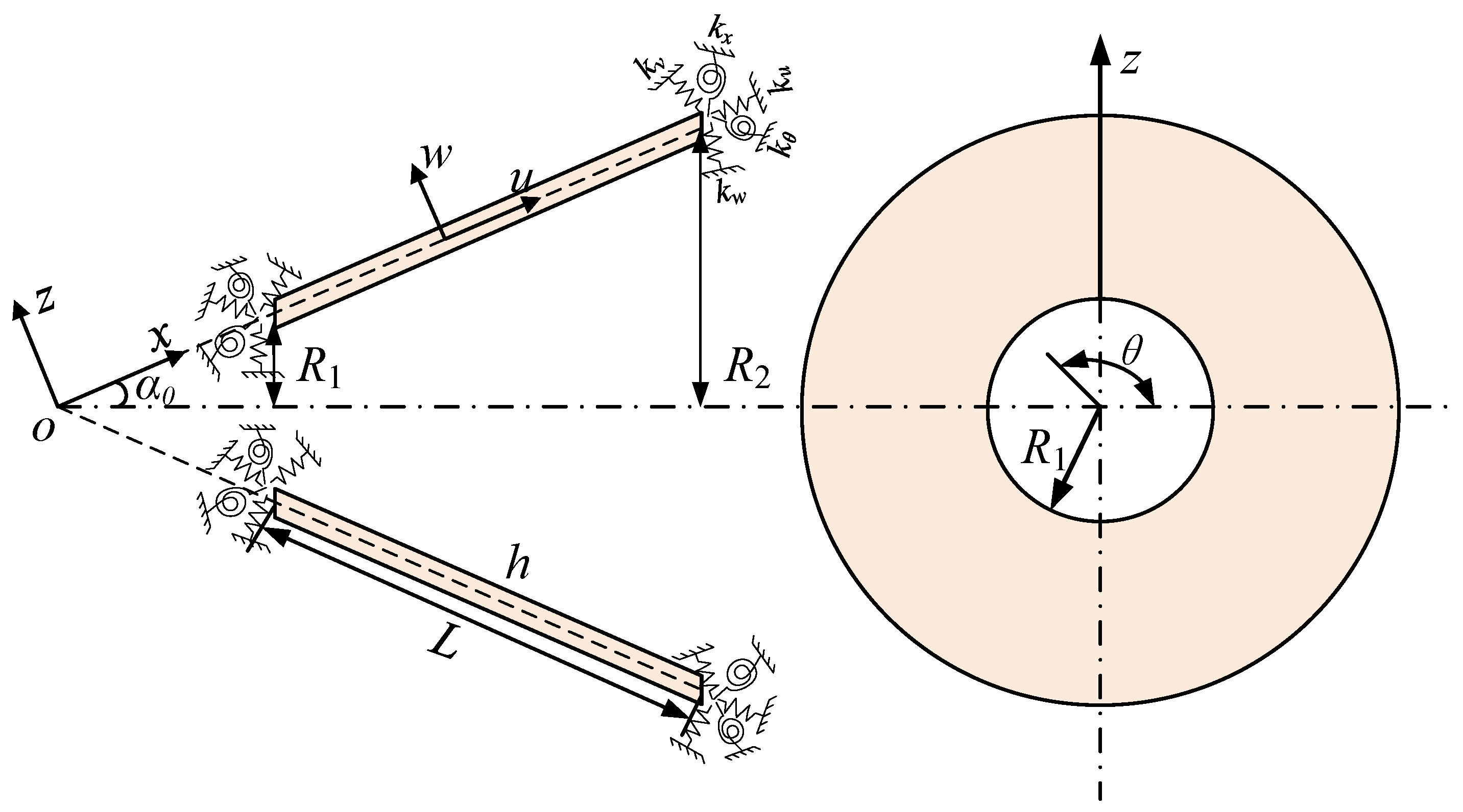
2.1. Theoretical Model of the Structure

The calculational analysis model of the conical shell structure is displayed in Figure 1, where L, h, α₀, R₁, and R₂ are the length, thickness, semi-vertex angle, and radius of both ends, respectively. The displacement of the conical shell structure is described by the cylindrical coordinate system, where the axial displacement is represented by x and the circumferential displacement is marked by θ. In addition, u, v, and w represent the corresponding axial, circumferential, and radial displacements. By introducing five series of spring stiffnesses ($k_u, k_v, k_w, k_x, \mathrm{and} k_{\theta }$) at the ends, the conical shell boundary conditions are obtained, and various spring stiffness values are set to simulate arbitrary boundary conditions. The conical shell structure is evenly segmented into H parts along the x direction, following the principles of the differential element approach. Section i can be connected to section i + 1 by a manual connection spring, with the spring stiffness set to infinity to indicate a large coupling effect between the segments.

2.2. Vibration Response Solution of the Rayleigh–Ritz Method

According to FSDT and generalized version of Hooke’s law, the constitutive equation of conical shell structures is as follows:

$$\left[\begin{array}{c}{N}_x^i\\ N_{\theta }^i\\ N_{x\theta }^i\\ M_{\theta }^i\\ M_{\theta }^i\\ M_{x\theta }^i\end{array}\right]=\left[\begin{array}{cccccc}{A}_{11}& A_{12}& 0& 0& 0& 0\\ A_{12}& A_{22}& 0& 0& 0& 0\\ 0& 0& A_{66}& 0& 0& 0\\ 0& 0& 0& D_{11}& D_{12}& 0\\ 0& 0& 0& D_{12}& D_{22}& 0\\ 0& 0& 0& 0& 0& D_{66}\end{array}\right]\left[\begin{array}{c}{\epsilon }_x^{0,i}\\ {\epsilon }_{\theta }^{0,i}\\ {\gamma }_{x\theta }^{0,i}\\ {\chi }_x^i\\ {\chi }_{\theta }^i\\ {\chi }_{x\theta }^i\end{array}\right]$$

(1)

$$\left\{\begin{array}{c}{Q}_{xz}^i\\ Q_{\theta z}^i\end{array}\right\}=\overline{\kappa }\left[\begin{array}{cc}{A}_{66}& 0\\ 0& A_{66}\end{array}\right]\left[\begin{array}{c}{\gamma }_{xz}^{0,i}\\ {\gamma }_{\theta z}^{0,i}\end{array}\right]$$

(2)

where $N_x^i$, $N_{\theta }^i$, $N_{x\theta }^i$, $M_x^i$, $M_{\theta }^i$, $M_{x\theta }^i$, $Q_{xz}^i$, and $Q_{\theta z}^i$ represent the respective forces, moments, and shear forces of ith segment. The shear correction factor is generally 5/6 [34,35].

The extensional stiffness coefficients and bending stiffness coefficients of the conical shell are denoted by $A_{ij},D_{ij}(i,j=1,2,6)$:

$$(A_{ij},D_{ij})={\displaystyle {\int }_{-h/2}^{h/2}{Q}_{ij}}(1,z^2)dz$$

(3)

where $Q_{ij}(i,j=1,2,6)$ is

$$Q_{11}=Q_{22}=\frac{E}{1-{\mu }^2}, Q_{12}=\frac{\mu E}{1-{\mu }^2}, Q_{66}=\frac{E}{2[1+\mu ]}$$

(4)

where E represents the elastic modulus and μ denotes Poisson’s ratio.

According to the FSDT, the conical shell’s structural strain energy can be calculated as follows:

$$U_V^i=\frac{1}{2}{\displaystyle {\iint }_S\left\{\begin{array}{l}{A}_{11}{\left(\frac{\partial u_0^i}{\partial x}\right)}^2+A_{22}{\left(\frac{1}{x\sin {\alpha }_0}\frac{\partial v_0^i}{\partial \theta }+\frac{u_0^i}{x}+\frac{w_0^i}{x\tan {\alpha }_0}\right)}^2+\\ A_{66}{\left(\frac{\partial v_0^i}{\partial x}+\frac{1}{x\sin {\alpha }_0}\frac{\partial u_0^i}{\partial \theta }-\frac{v_0^i}{x}\right)}^2+\overline{\kappa }{A}_{66}{\left(\frac{\partial w_0^i}{\partial x}+{\varphi }_x^i\right)}^2+\\ 2A_{12}\left(\frac{\partial u_0^i}{\partial x}\right)\left(\frac{1}{x\sin {\alpha }_0}\frac{\partial v_0^i}{\partial \theta }+\frac{u_0^i}{x}+\frac{w_0^i}{x\tan {\alpha }_0}\right)+\\ \overline{\kappa }{A}_{66}{\left(\frac{1}{x\sin {\alpha }_0}\frac{\partial w_0^i}{\partial \theta }-\frac{v_0^i}{x\tan {\alpha }_0}+{\varphi }_{\theta }^i\right)}^2+\\ D_{11}{\left(\frac{\partial {\varphi }_x^i}{\partial x}\right)}^2+2D_{12}\left(\frac{\partial {\varphi }_x^i}{\partial x}\right)\left(\frac{1}{x\sin {\alpha }_0}\frac{\partial {\varphi }_{\theta }^i}{\partial \theta }+\frac{{\varphi }_x^i}{x}\right)+\\ D_{22}{\left(\frac{1}{x\sin {\alpha }_0}\frac{\partial {\varphi }_{\theta }^i}{\partial \theta }+\frac{{\varphi }_x^i}{x}\right)}^2+D_{66}{\left(\frac{1}{x\sin {\alpha }_0}\frac{\partial {\varphi }_x^i}{\partial \theta }+\frac{\partial {\varphi }_{\theta }^i}{\partial x}-\frac{{\varphi }_{\theta }^i}{x}\right)}^2\end{array}\right\}}dS$$

(5)

By introducing five sets of springs to simulate the boundary of the conical shell, the boundary potential energy U_b of the structure is

$$U_b=\frac{1}{2}{\displaystyle {\int }_{-h/2}^{h/2}{\displaystyle {\int }_0^{2\pi }\left\{\begin{array}{l}{\left[\begin{array}{l}{k}_{u,x0}{u}_0^2+k_{v,x0}{v}_0^2+\\ k_{w,x0}{w}_0^2+k_{x,x0}{\varphi }_x^2+\\ k_{\theta ,x0}{\varphi }_{\theta }^2\end{array}\right]}_{R=R_1}+\\ {\left[\begin{array}{l}{k}_{u,xL}{u}_0^2+k_{v,xL}{v}_0^2+\\ k_{w,xL}{w}_0^2+k_{x,xL}{\varphi }_x^2+\\ k_{\theta ,xL}{\varphi }_{\theta }^2\end{array}\right]}_{R=R_2}\end{array}\right\}x\sin {\alpha }_{0}d\theta }}dz$$

(6)

The connecting spring potential energy between different substructures is

$$U_s^i=\frac{1}{2}{\displaystyle {\int }_{-h/2}^{h/2}{\displaystyle {\int }_0^{2\pi }{\left\{\begin{array}{l}{k}_u{\left(u_0^i-u_0^{i+1}\right)}^2+k_v{\left(v_0^i-v_0^{i+1}\right)}^2+\\ k_w{\left(w_0^i-w_0^{i+1}\right)}^2+k_x{\left({\varphi }_x^i-{\varphi }_x^{i+1}\right)}^2+\\ k_{\theta }{\left({\varphi }_{\theta }^i-{\varphi }_{\theta }^{i+1}\right)}^2\end{array}\right\}}_{i,i+1}x\sin {\alpha }_{0}d\theta }}dz$$

(7)

Then, the total potential energy U_BS is

$$U_{BS}=U_b+{\displaystyle \sum _{i=1}^{H-1}{U}_s^i}$$

(8)

The kinetic energy function Tⁱ is

$$T^i==\frac{1}{2}{\displaystyle {\iint }_S\left\{\begin{array}{l}{I}_1\left[{\left(\frac{\partial u_0^i}{\partial t}\right)}^2+{\left(\frac{\partial v_0^i}{\partial t}\right)}^2+{\left(\frac{\partial w_0^i}{\partial t}\right)}^2\right]+\\ I_3\left[{\left(\frac{\partial {\varphi }_x^i}{\partial t}\right)}^2+{\left(\frac{\partial {\varphi }_{\theta }^i}{\partial t}\right)}^2\right]+\\ 2I_2\left[\left(\frac{\partial u_0^i}{\partial t}\right)\left(\frac{\partial {\varphi }_x^i}{\partial t}\right)+\left(\frac{\partial v_0^i}{\partial t}\right)\left(\frac{\partial {\varphi }_{\theta }^i}{\partial t}\right)\right]\end{array}\right\}}dS$$

(9)

Among them,

$$(I_1,I_2,I_3)=\underset{-h/2}{\overset{h/2}{\int }}\rho (z)(1,z,z^2)dz$$

(10)

The ith conical shell segment’s work performed by an external excitation load is as follows:

$$W^i={\displaystyle \int f_{w,i}{w}_{i}dx}$$

(11)

where f_w,i denotes the concentrated force acting in the w direction towards the surface.

The displacement functions of the structure are created using Jacobi orthogonal polynomials and Fourier series. Each function component of the structure can be shown as follows:

$$\left\{\begin{array}{l}{u}_0={\displaystyle \sum _{m=0}^M{\displaystyle \sum _{n=0}^N{P}_m^{(\alpha ,\beta )}}}(x)\left[A_m\cos (n\theta )+B_m\sin (n\theta )\right]e^{i\omega t}\\ v_0={\displaystyle \sum _{m=0}^M{\displaystyle \sum _{n=0}^N{P}_m^{(\alpha ,\beta )}}}(x)\left[C_m\sin (n\theta )+D_m\cos (n\theta )\right]e^{i\omega t}\\ w_0={\displaystyle \sum _{m=0}^M{\displaystyle \sum _{n=0}^N{P}_m^{(\alpha ,\beta )}}}(x)\left[E_m\cos (n\theta )+F_m\sin (n\theta )\right]e^{i\omega t}\\ {\varphi }_x={\displaystyle \sum _{m=0}^M{\displaystyle \sum _{n=0}^N{P}_m^{(\alpha ,\beta )}}}(x)\left[G_m\cos (n\theta )+H_m\sin (n\theta )\right]e^{i\omega t}\\ {\varphi }_{\theta }={\displaystyle \sum _{m=0}^M{\displaystyle \sum _{n=0}^N{P}_m^{(\alpha ,\beta )}}}(x)\left[I_m\sin (n\theta )+J_m\cos (n\theta )\right]e^{i\omega t}\end{array}\right.$$

(12)

where A_m, B_m, C_m, D_m, E_m, F_m, G_m, H_m, I_m, and J_m, represent unknown coefficients, axial and circumferential wave numbers are represented by n and m, and N and M are the highest degrees of n and m.

The conical shell structure’s overall Lagrange energy function is described as

$$\mathcal{L}={\displaystyle \sum _1^{N-1}\left(W^i+T^i-U_V^i\right)}-U_{BS}$$

(13)

By applying the Rayleigh–Ritz method, the variational form of L is obtained:

$$\frac{\partial \mathcal{L}}{\partial \vartheta }=0; \vartheta =A_m, B_m, C_m, D_m, E_m, F_m, G_m, H_m, I_m, J_m$$

(14)

Rayleigh damping is introduced, and the time domain vibration response is solved based on the Newmark-β integration approach.

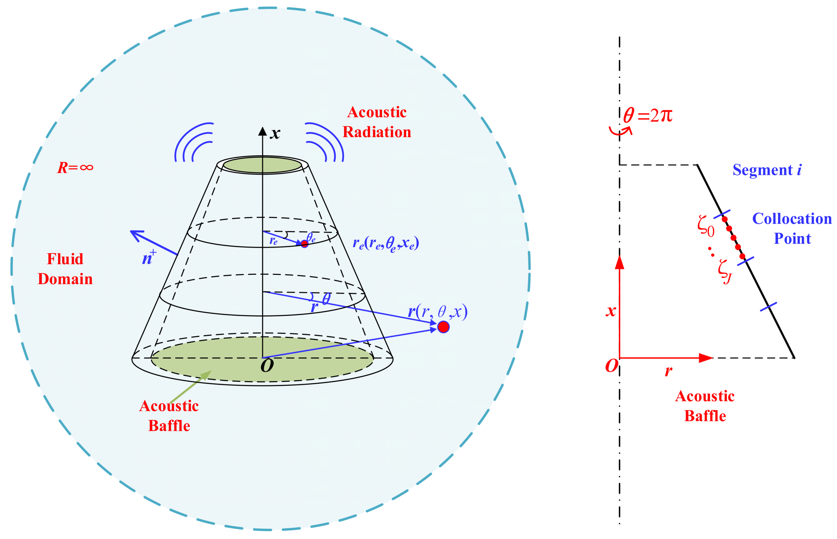
2.3. Acoustic Response Solution Based on the Boundary Element Method

The time domain BEM can automatically satisfy Sommerfeld’s far-field radiation conditions. Figure 2 shows the coordinate system of external acoustic radiation from a conical shell.

When applying the Kirchhoff boundary integral formulation in the time domain, the sound pressure p(r, t) at any field point r can be stated as

$$\Re (\mathit{r})p(\mathit{r},t)+{\displaystyle {\iint }_{\text{ϒ}}\left({\displaystyle {\int }_0^{t}G(\mathit{r},{\mathit{r}}_{\mathit{e}},t,\tau )}\frac{\partial p({\mathit{r}}_{\mathit{e}},\tau )}{\partial n^{+}}\right)}\mathrm{d}\text{ϒ}={\displaystyle {\iint }_{\text{ϒ}}\left({\displaystyle {\int }_0^{t}p({\mathit{r}}_{\mathit{e}},\tau )G^{*}(\mathit{r},{\mathit{r}}_{\mathit{e}},t,\tau )}\right)}\mathrm{d}\text{ϒ}$$

(15)

where the vector r_e represents the source point, while the normal derivatives and basic solutions of the sound field wave equation in the time domain are denoted by $G^{*}\left(r,r_e,t,\tau \right), G\left(r,r_e,t,\tau \right)$. The normal direction outside the boundary of the shell surface is represented by n⁺, and the sound source dϒ can be identified at the sound field boundary ϒ.

The $\Re (r)$ coefficients are defined as follows:

$$\Re (r)=\left(\begin{array}{l}1 r\in \Omega \\ \frac{1}{2} r\in \text{ϒ}\\ 0 r\notin \Omega \mathrm{and} r\notin \text{ϒ}\end{array}\right.$$

(16)

The time domain boundary integral equation is numerically discretized, in which the time axis is equally split into N_t parts $(t_n=n_t\Delta t,n_t=0, 1,\dots N_t)$. Time interpolation is conducted on the physical quantities of the sound field using the mth time step, and the following results are obtained:

$$p^m({\mathit{r}}_{\mathit{e}},\tau )={\displaystyle \sum _{i=1}^I{T}_i^m}(\tau )p_i^m({\mathit{r}}_{\mathit{e}}), q^m({\mathit{r}}_{\mathit{e}},\tau )=\frac{\partial p^m({\mathit{r}}_{\mathit{e}},\tau )}{\partial n^{+}}={\displaystyle \sum _{i=1}^I{\overline{T}}_i^m}(\tau )q_i^m({\mathit{r}}_{\mathit{e}})$$

(17)

where $q_i^m(r_e)$ and $p_i^m(r_e)$ are the normal derivative and the spatial distribution functions of the sound pressure, respectively. i is the order of the mth step of the time interpolation function, and $T_i^m(\tau )$ and ${\overline{T}}_i^m(\tau )$ represent the time interpolation functions. If $I=2$, then $T_i^m(\tau )$ and ${\overline{T}}_i^m(\tau )$ take the same time interpolation function, and we obtain

$$\begin{array}{l}{T}_1^m(\tau )={\overline{T}}_1^m(\tau )=1-\tau /\Delta t\\ T_2^m(\tau )={\overline{T}}_2^m(\tau )=\tau /\Delta t\end{array}$$

(18)

Given that the fundamental solution is time-translation invariant, the boundary integral equation of the discrete time domain sound field is as follows:

$$\Re (\mathit{r})p(\mathit{r},t_{n_t})+{\displaystyle \sum _{m=1}^{N_t}{\displaystyle \sum _{i=1}^I{\displaystyle {\iint }_{\text{ϒ}}\left({\tilde{G}}_{\left(n_t-m+1\right)\left(1\right)}^i(\mathit{r},{\mathit{r}}_{\mathit{e}})q_i^m({\mathit{r}}_{\mathit{e}})\right)}}}d\text{ϒ}={\displaystyle \sum _{m=1}^{N_t}{\displaystyle \sum _{i=1}^I{\displaystyle {\iint }_{\text{ϒ}}\left(H_{\left(n_t-m+1\right)\left(1\right)}^i(\mathit{r},{\mathit{r}}_{\mathit{e}})p_i^m({\mathit{r}}_{\mathit{e}})\right)}}}d\text{ϒ}$$

(19)

In the cylindrical coordinate system, Fourier series are used to transform the two-dimensional sound field boundary integral equation into a one-dimensional sound field boundary integral equation along the circular direction. The sound field boundary integral equation is given by

$$\left\{\begin{array}{l}{p}_i^m(\mathit{r})={\displaystyle \sum _{n=0}^N\left[p_{i,n}^s(r,n,x)\sin n\theta +p_{i,n}^c(r,n,x)\cos n\theta \right]}\\ p_i^m({\mathit{r}}_{\mathit{e}})={\displaystyle \sum _{n=0}^N\left[p_{i,n}^s(r_e,n,x_e)\sin n{\theta }_e+p_{i,n}^c(r_e,n,x_e)\cos n{\theta }_e\right]}\end{array}\right.$$

(20)

where the variables $p_{i,n}^c$ and $p_{i,n}^s$ indicate the Fourier series expansion coefficients for the boundary sound pressure normal derivative. Also, the normal derivatives of Green’s function and its expansion are as follows:

$$\left\{\begin{array}{l}{\tilde{G}}_{\left(n_t-m+1\right)\left(1\right)}^i(\mathit{r},{\mathit{r}}_{\mathit{e}})=\left\{\begin{array}{l}\frac{1}{\pi }{\displaystyle \sum _{n=0}^N{G}_{\left(n_t-m+1\right)\left(1\right)n}^i\left[\begin{array}{l}\sin n\theta \sin n{\theta }_e+\\ \cos n\theta \cos n{\theta }_e\end{array}\right]}, \frac{r_s}{c}\le t_{n_t}\le \frac{r_s}{c}+\Delta t\\ 0,\hspace{1em}\hspace{1em}\hspace{1em}\hspace{1em}\hspace{1em}\hspace{1em}\hspace{1em}\hspace{1em}\hspace{1em}\hspace{1em}\hspace{1em}\hspace{1em}\mathrm{other}\end{array}\right. \\ H_{\left(n_t-m+1\right)\left(1\right)}^i(\mathit{r},{\mathit{r}}_{\mathit{e}})=\left\{\begin{array}{l}\frac{1}{\pi }{\displaystyle \sum _{n=0}^N{H}_{\left(n_t-m+1\right)\left(1\right)n}^i\left[\begin{array}{l}\sin n\theta \sin n{\theta }_e+\\ \cos n\theta \cos n{\theta }_e\end{array}\right]}, \frac{r_s}{c}\le t_{n_t}\le \frac{r_s}{c}+\Delta t\\ 0,\hspace{1em}\hspace{1em}\hspace{1em}\hspace{1em}\hspace{1em}\hspace{1em}\hspace{1em}\hspace{1em}\hspace{1em}\hspace{1em}\hspace{1em}\hspace{1em}\mathrm{other}\end{array}\right. \end{array}\right.$$

(21)

The coefficients $G_{\left(n_t-m+1\right)\left(1\right)n}^i$ and $H_{\left(n_t-m+1\right)\left(1\right)n}^i$ are expressed as

$$\left\{\begin{array}{l}{G}_{\left(n_t-m+1\right)\left(1\right)n}^i={\displaystyle \underset{0}{\overset{2\pi }{\int }}\frac{1}{4\pi r_s}{\overline{T}}_i(t_{n_t}-\frac{r_s}{c})}\cos n\varphi \mathrm{d}\varphi \\ H_{\left(n_t-m+1\right)\left(1\right)n}^i={\displaystyle \underset{0}{\overset{2\pi }{\int }}-\frac{1}{4\pi r_s^2}\frac{\partial r}{\partial n}\left[T_i(t_{n_t}-\frac{r_s}{c})+\frac{r_s}{c}{\dot{T}}_i(t_{n_t}-\frac{r_s}{c})\right]}\cos n\varphi \mathrm{d}\varphi \end{array}\right.$$

(22)

where

$$\varphi ={\theta }_e-\theta ,{\theta }_e=\varphi +\theta ,\mathrm{d}{\theta }_e=\mathrm{d}\varphi$$

(23)

Based on the first kind of Chebyshev polynomial discrete sound field boundary, the configuration point is set on the boundary element to ensure that the sound field boundary and the structure boundary match, and then the Fourier sound pressure coefficient is expanded as follows:

$$\left\{\begin{array}{l}{p}_{i,n}^s={\displaystyle \sum _{j=0}^J{T}_j\left(\xi \right)p_{i,n,j}^s}=T_p\left(\xi \right)p_{i,n}^s\\ p_{i,n}^c={\displaystyle \sum _{j=0}^J{T}_j\left(\xi \right)p_{i,n,j}^c}=T_p\left(\xi \right)p_{i,n}^c\end{array}\right.$$

(24)

The jth Chebyshev polynomial of the first class is denoted by T_j (ξ). J denotes the maximum degree of j. The improved time domain boundary integral equation is calculated by inserting Equations (20)–(24) into Equation (19).

$$\left\{\begin{array}{l}\Re (\mathit{r})T_p\left(\mathit{r}\right)p_{i,n}^s+{\displaystyle \sum _{e=1}^N{\displaystyle \sum _{m=1}^{N_t}{\displaystyle \sum _{i=1}^I{\displaystyle {\int }_{l_e}\left[{\tilde{G}}_{\left(n_t-m+1\right)\left(1\right)}^i(\mathit{r},{\mathit{r}}_{\mathit{e}})T_p{r}_e\left(\xi \right)\left|J_{\xi }\right|\mathrm{d}\xi \right]}}}}{q}_{i,n}^s\\ ={\displaystyle \sum _{e=1}^N{\displaystyle \sum _{m=1}^{N_t}{\displaystyle \sum _{i=1}^I{\displaystyle {\int }_{l_e}\left[H_{\left(n_t-m+1\right)\left(1\right)}^i(\mathit{r},{\mathit{r}}_{\mathit{e}})T_p{r}_e\left(\xi \right)\left|J_{\xi }\right|\mathrm{d}\xi \right]}}}}{p}_{i,n}^s\\ \Re (\mathit{r})T_p\left(\mathit{r}\right)p_{i,n}^c+{\displaystyle \sum _{e=1}^N{\displaystyle \sum _{m=1}^{N_t}{\displaystyle \sum _{i=1}^I{\displaystyle {\int }_{l_e}\left[{\tilde{G}}_{\left(n_t-m+1\right)\left(1\right)}^i(\mathit{r},{\mathit{r}}_{\mathit{e}})T_p{r}_e\left(\xi \right)\left|J_{\xi }\right|\mathrm{d}\xi \right]}}}}{q}_{i,n}^c\\ ={\displaystyle \sum _{e=1}^N{\displaystyle \sum _{m=1}^{N_t}{\displaystyle \sum _{i=1}^I{\displaystyle {\int }_{l_e}\left[H_{\left(n_t-m+1\right)\left(1\right)}^i(\mathit{r},{\mathit{r}}_{\mathit{e}})T_p{r}_e\left(\xi \right)\left|J_{\xi }\right|\mathrm{d}\xi \right]}}}}{p}_{i,n}^c\end{array}\right.$$

(25)

where $\left|J_{\xi }\right|$ and T_p are the Jacobian matrix of coordinate transformation and a vector composed of orthogonal polynomials, respectively. Each boundary element has (J + 1) collocation points, which are precisely situated at the zero of the first Chebyshev polynomial.

$${\xi }_j=\cos \left(\frac{2j-1}{2(J+1)}\pi \right),j=1,2,\dots ,(J+1)$$

(26)

At the radiation surface of the shell,

$$\frac{\partial p({\mathit{r}}_{\mathit{e}},t)}{\partial n^{+}}=-{\rho }_0{\left[{\ddot{w}}_j({\mathit{r}}_{\mathit{e}},t)\right]}_{r=R}$$

(27)

where ρ₀ is the fluid density, and ${\ddot{w}}_j({\mathit{r}}_{\mathit{e}},t)$ denotes the normal acceleration of the conical shell, which is solved by the Newmark-β integral method and Equation (12). Equations (25) and (26) are jointly expressed in matrix form as:

$$\mathit{C}{p}^{n,l}={\displaystyle \sum _{m=1}^{N_t}{\displaystyle \sum _{i=1}^I{\tilde{\mathit{G}}}_{\left(n_t-m+1\right)\left(1\right)}^i}}{\ddot{\mathit{w}}}_i^n+{\displaystyle \sum _{m=1}^{N_t}{\displaystyle \sum _{i=1}^I{\mathit{H}}_{\left(n_t-m+1\right)\left(1\right)}^i{p}_i^n}}$$

(28)

where ${\ddot{\mathit{w}}}_i^n$ and $p_i^n$ stand for the acceleration and sound pressure, respectively, and ${\tilde{\mathit{G}}}_{\left(n_t-m+1\right)\left(1\right)}^i$ and ${\mathit{H}}_{\left(n_t-m+1\right)\left(1\right)}^i$ represent the coefficient matrix. The generalized sound pressure vector on the lth boundary element is represented by $p^{n,l}$.

3. Convergence Discussion and Validity Verification

3.1. Computational Model

In this section, through a discussion of the vibration results and the acoustic radiation of conical shells, the convergence and accuracy of the presented method are verified. The conical shell structure dimensions are as follows: ${\alpha }_0=\mathsf{\pi }/6$, R₁ = 0.5 m, L = 3 m, and h = 0.008 m. The material and convergence parameters are ρ = 7850 kg/m³, E = 210 Gpa, μ = 0.3, M = N = 8, α = β = 1, H = 4, and J = 4. In

Table 1. The virtual spring stiffness values of complex boundary conditions.

Type	Wire Spring Stiffness ku = kv = kw (N/m)	Rotating Spring Stiffness kx = kθ (N·m/rad)
Clamped—C	1015	1015
Simply Support—S	1015	0
Free—F	0	0
Elastic—E	108	10

, virtual spring stiffness values for both end boundaries of the conical shell structure are presented [36,37].

Figure 3 shows the selected triangular pulse excitation load. The excitation point is (0.25L, 0, R), the vibration examination point is (0.75L, 0, R), and the acoustic examination point is (0.5L, 0, 2).

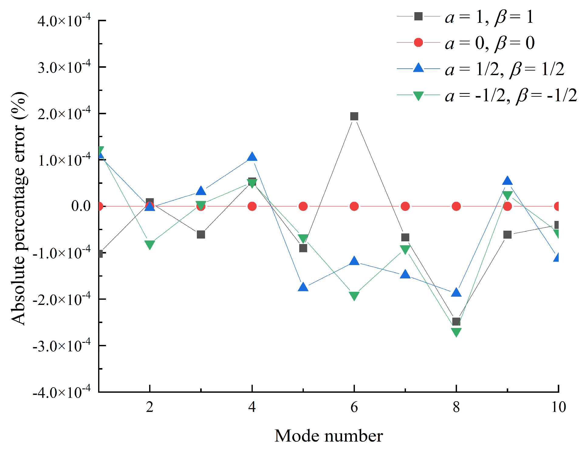
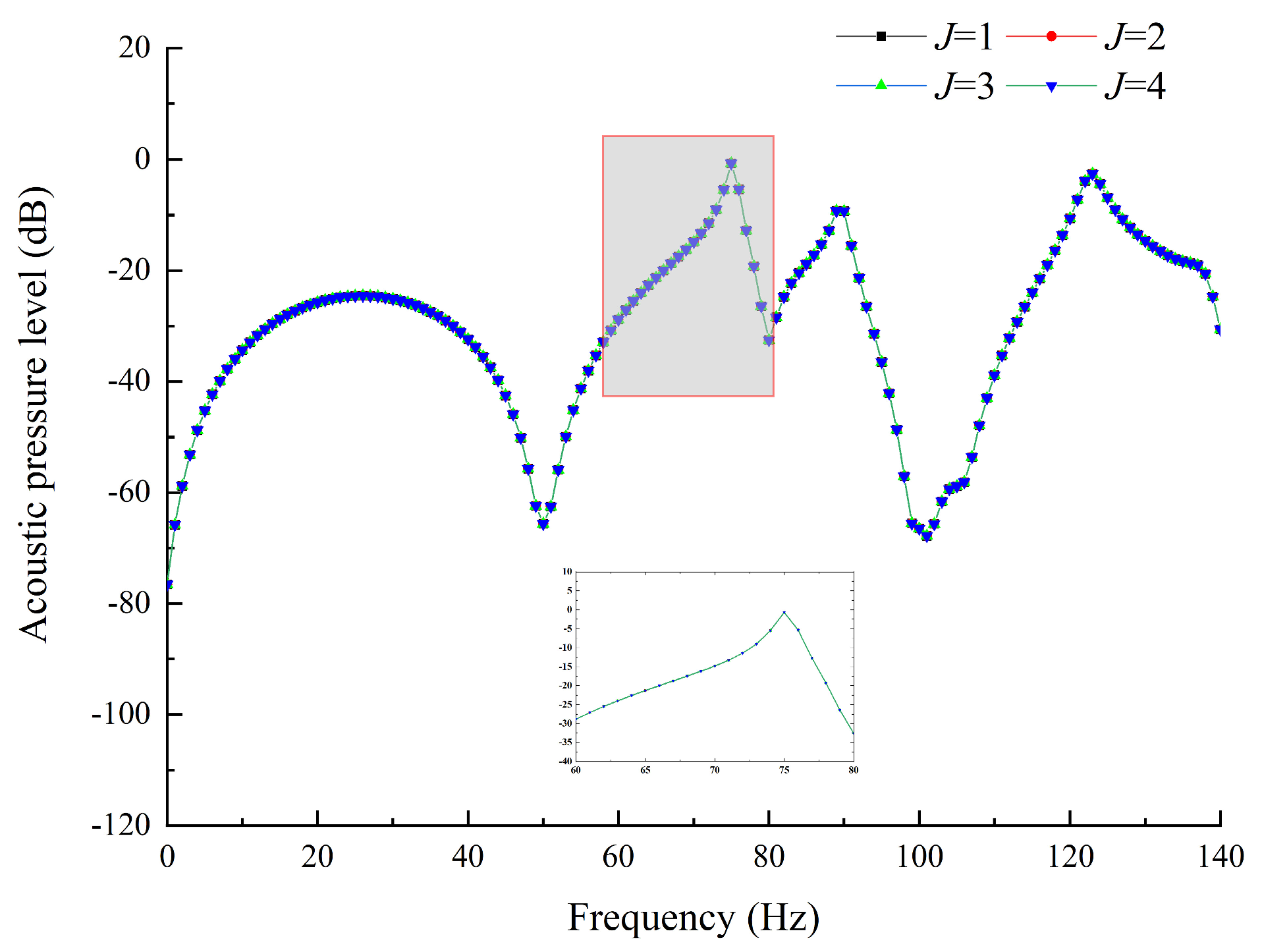
3.2. Convergence Discussion

Under the simply supported edges on both sides of a conical shell, the convergence of the method is discussed. Similarly, the conclusion of the discussion is consistent with the arbitrary boundary conditions of conical shells. According to the abovementioned theoretical derivation, the energy function of the structure is established based on the differential element method, and the arbitrary boundary is simulated using the artificial spring technique. Therefore, convergence depends on the displacement tolerance function, the number of segments, Jacobi parameters, and the sound pressure function.

Figure 4 shows the effects of different segment numbers H and displacement allowable function truncation numbers M and N on the calculation results of the natural frequency of the conical shell when the Jacobi parameters are as follows: α = 1 and β = 1. As can be observed, with the addition of the truncation number of the displacement tolerance function and the number of segments, the natural frequency of the conical shell structure tends to converge gradually. The free vibration results of the conical shell converge and agree with the FEM results when the truncation coefficients reach H ≥ 3, M ≥ 6, and N ≥ 6 However, the order of the matrix calculation will increase with an increase in convergence parameters. On the basis of ensuring calculation accuracy, the subsequent analysis of the number of segments and the truncation number of the displacement tolerance function is chosen as follows: H = 4, M = 8, and N = 8.

In terms of the values of the Jacobi parameters, the natural frequencies under α = 0 and β = 0 are taken as reference values. Figure 5 displays the absolute errors of structural natural frequencies under different Jacobi parameters.

Figure 5 shows that the maximum absolute percentage error of the different Jacobi parameters α and β under simply supported boundary conditions is less than 3 × 10⁻⁶, indicating that the selection of Jacobi parameters has little effect on the vibration responses of conical shell structures.

Figure 6 shows the acoustic radiation under different sound pressure truncation functions J. The analysis results show that the acoustic pressure level of the conical shell converges rapidly and stably with an increase in the truncation number of the sound pressure function J, when the calculation parameters of the structural vibration response are fixed. By the same token, the sound pressure truncation function is chosen as follows: J = 4.

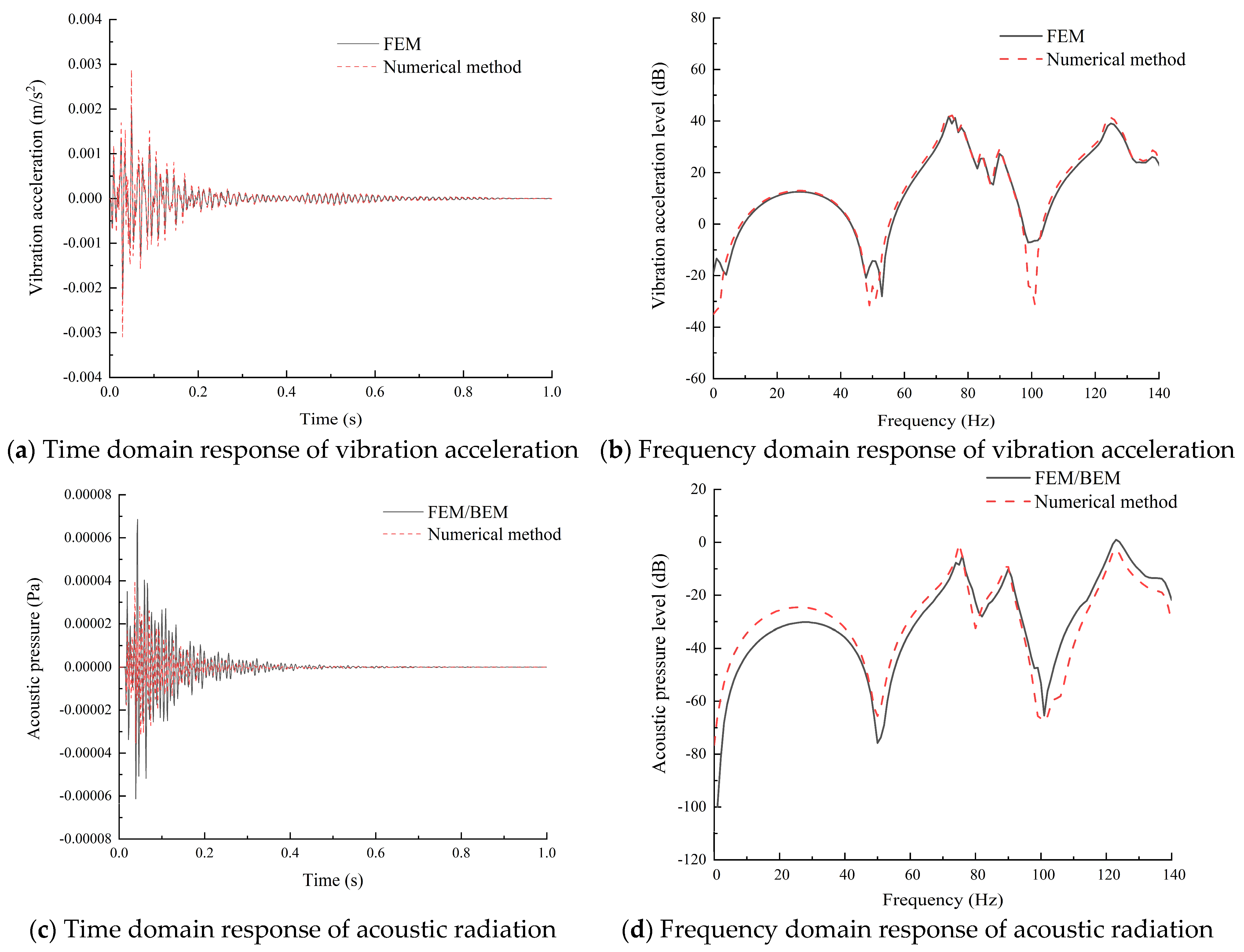
3.3. Validity Verification

In order to verify the effectiveness of the Jacobi–Ritz boundary element method, a single triangular pulse load is applied, as seen in Figure 3a. The number of segments, the displacement tolerance function, the Jacobi parameters, and the truncation number of the sound pressure function are chosen as follows: H = 4, M = 8, N = 8, α = 1, β = 1, and J = 4; the boundary conditions are simply supported. Figure 7 exhibits the comparison of the vibro-acoustic responses between the proposed method and the FEM/BEM in the time and frequency domains.

From the abovementioned comparison curves, the vibro-acoustic responses calculated using the proposed method in the time–frequency domain are in agreement with FEM/BEM. The difference may be due to the inconsistency of matching algorithms between sound field nodes and structural nodes at the fluid-solid interface. There is a small error between the proposed method and the FEM/BEM, which verifies the effectiveness of the Jacobi–Ritz boundary element method.

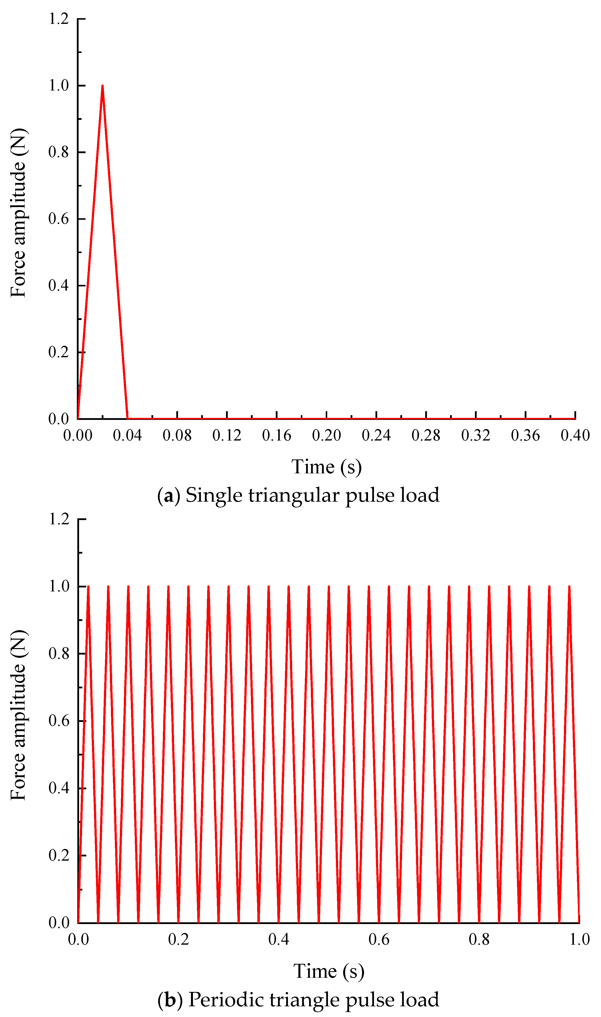
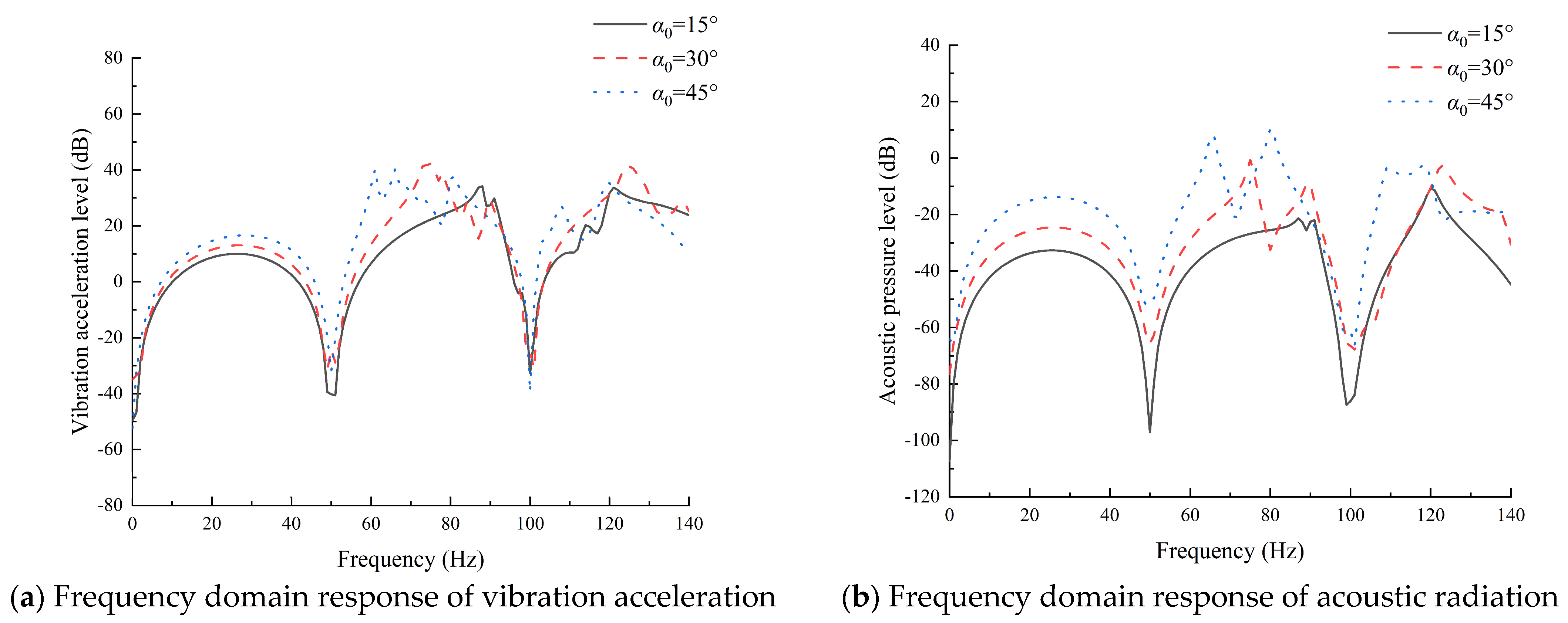
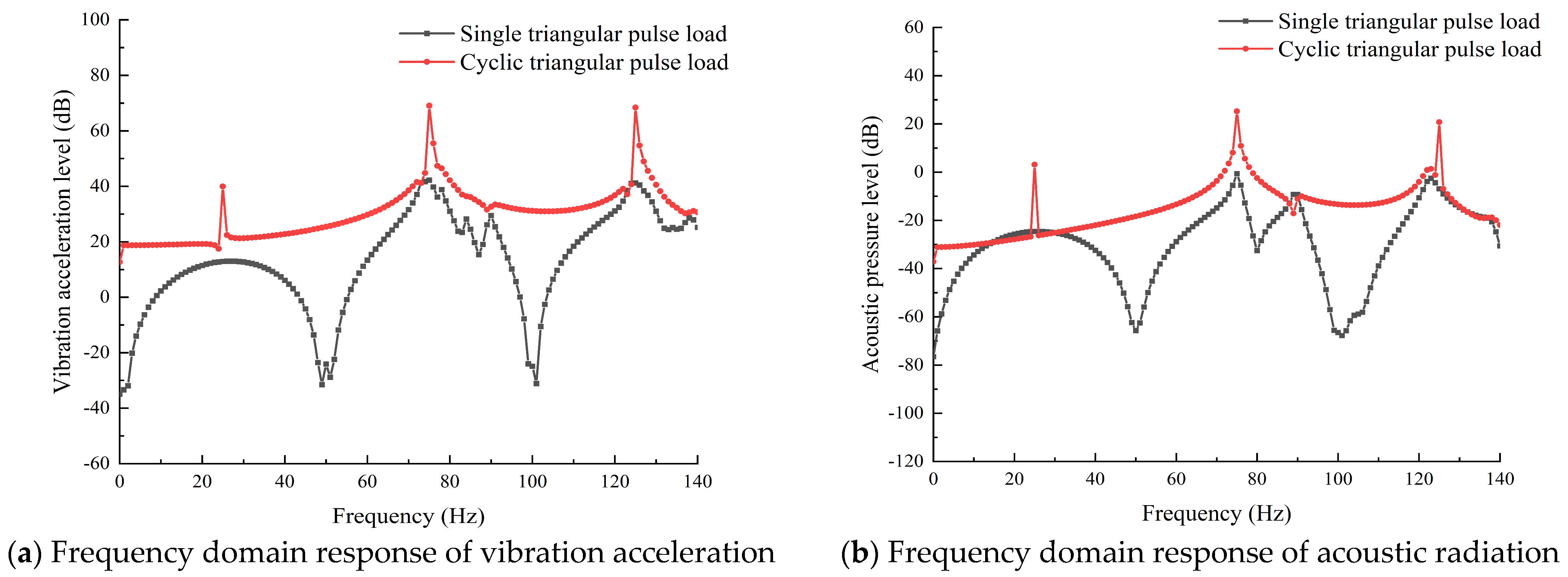
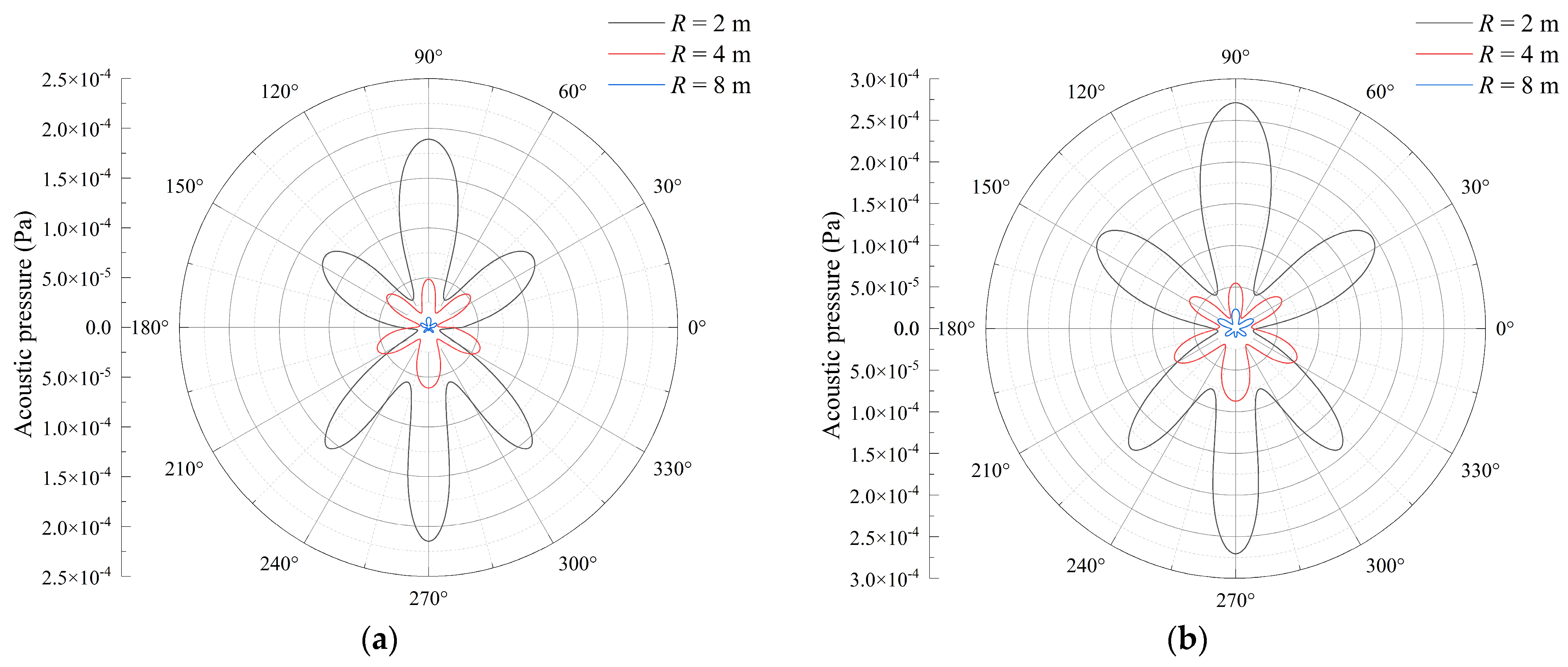
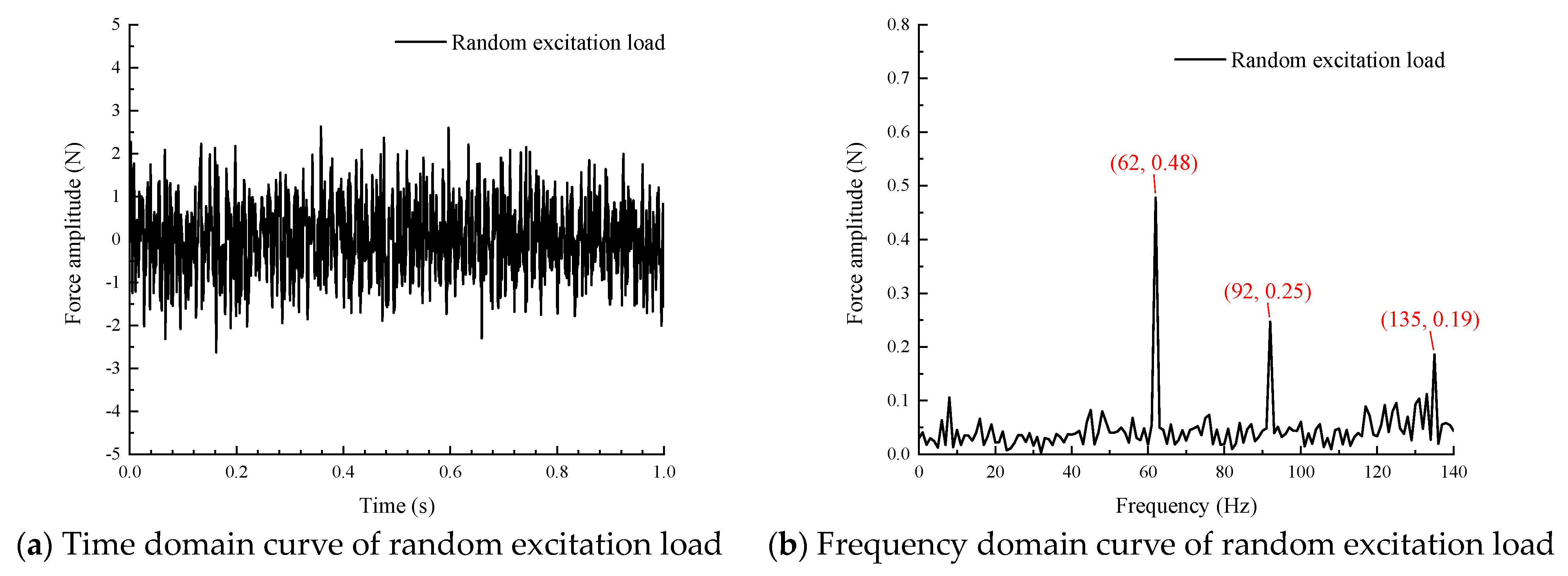
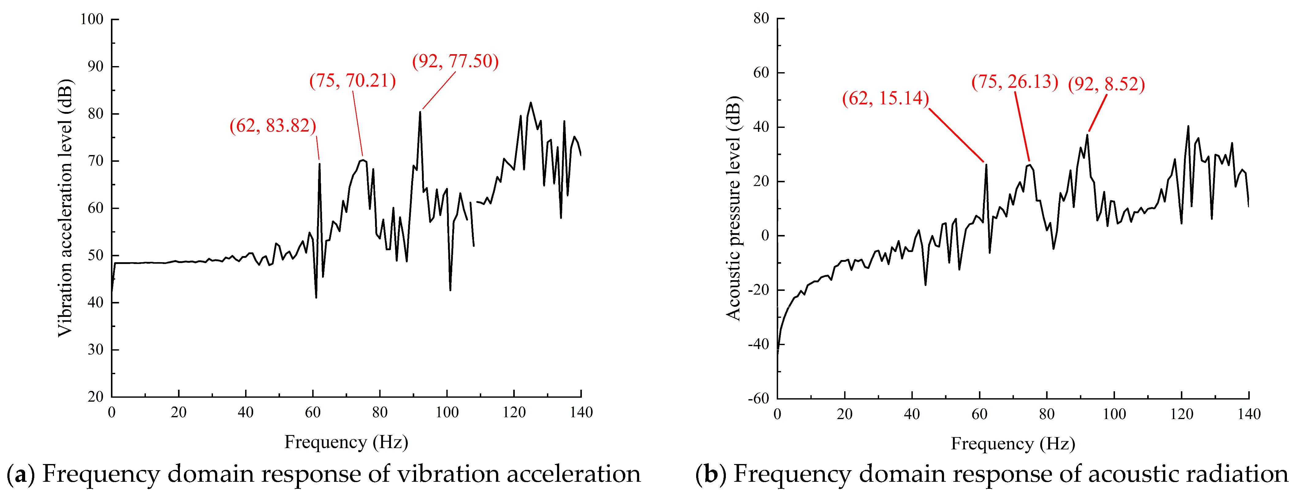
4. Results and Discussion

According to the spring stiffness values shown in Table 1, take the single triangular pulse load shown in Figure 3a as the excitation. Under various boundary conditions, Figure 8 shows the time–frequency response curve of vibration acceleration and acoustic radiation of the structure.

Figure 8 shows that the change in boundary conditions has a great effect on the acoustic radiation response of the forced vibration of the structure. The “SF” causes the value of the forced vibration response to peak at 13 Hz and 23 Hz compared with the other three boundary conditions “CC”, “SS”, and “SC”. Because the “SF” boundary condition is compared with other boundary conditions, there are inherent modes at 13.3 Hz and 22.5 Hz. In addition, the fixed boundary condition constrains the stiffness value of the rotating spring compared with the simply supported boundary condition, but it has a smaller influence on the natural frequency of the conical shell structure, so the difference in the resonance peak frequency of the acoustic result under the other three boundary conditions is small.

In order to discuss the vibration and sound radiation characteristics of conical shells at different semi-vertex angles, the structural parameters, such as the length and thickness of the structure, are fixed, and the semi-vertex angle of the structure is adjusted. Figure 9 exhibits the frequency domain response curve of the vibro-acoustic results of the conical shell at various semi-vertex angles.

Figure 9 demonstrates that altering the semi-vertex angles of the conical shell has a substantial impact on the acoustic radiation resulting from forced vibration. As the semi-vertex angle of the structure grows, the acoustic radiation response of the forced vibration increases gradually, and the peak frequency moves to the left mainly because the structural stiffness decreases with an increase in the semi-vertex angle, and its natural frequency moves to a low frequency.

In order to explore the influence of acoustic radiation characteristics on the forced vibration of the structure under various excitation loads, a single triangular pulse and a periodic triangular pulse with a pulse width of 0.02 s and an amplitude of 1 N are selected, as shown in Figure 3, and the duration of each pulse is 1 s. Figure 10 shows the vibro-acoustic characteristic curves under two forms of excitation.

Figure 10 shows that, in addition to the natural mode of the structure, the influence of the form of excitation load on the vibration response and acoustic radiation of the structure is also more significant. Compared with the single triangular pulse load, the periodic triangular pulse load causes the vibration response and radiation noise to peak at the frequency doubling of 25 Hz, 75 Hz, 125 Hz, and so on, mainly because the periodic triangular pulse load has the excitation peak value and its frequency doubling component at this frequency. In order to reflect the transmission of radiated noise and the sound pressure distribution of the conical shell under a characteristic frequency, the radiation directivity patterns of radiated sound at circumferential distances of 2 m, 4 m, and 8 m under a periodic triangular wave load at 0.5 s and 0.7 s and at frequencies of 75 Hz and 125 Hz are shown in Figure 11.

Figure 11 shows that the acoustic radiation is symmetrically distributed in the connection line between 90° (the excitation direction of the force) and 270° in the time and frequency domains. In addition, the circumferential sound pressure distribution at the peak of the vibration response of the conical shell is closely related to the vibration mode shape. In order to explore the influence of the randomness of the excitation load on the vibro-acoustic response of the conical shell, the random excitation load is applied at the excitation point (0.25 L, 0, R). Figure 12 shows the random excitation load curve. Figure 13 displays the structural vibration response and the acoustic radiation curve under the random excitation load.

Figure 13 shows that the vibration response of the conical shell structure under random excitation has peak values at 62 Hz, 92 Hz, and 75 Hz; 62 Hz and 92 Hz are caused by the excitation load at this frequency peak, while 75 Hz is caused by the strong characteristic line spectrum of the conical shell structure under a natural frequency of 75.4 Hz.

5. Conclusions

In light of the Jacobi–Ritz boundary element method, this paper describes the vibro-acoustic behaviors of conical shells under various boundary conditions. The analytical model was constructed by utilizing the differential element method and artificial spring technology. The proposed method ensured convergence and efficacy through the incorporation of the Fourier series and Jacobi polynomials. In addition, the vibration result was determined using the Newmark-β integration method, and the external acoustic field was calculated using the Kirchhoff boundary integral formulation in the time domain. Additionally, the acoustic model of forced vibration in the time domain was established for the conical shell and took into account the external excitation operating on its surface. The proposed method was demonstrated to possess high accuracy and reliability when compared to the coupled FEM/BEM. Notably, this method needs to be further extended to the transient vibro-acoustic radiation analysis of composite structures. The main conclusions are as follows:

• Under simply supported boundary conditions, the results of the Jacobi–Ritz boundary element method were in agreement with the coupled FEM/BEM, which has advantages such as fast calculation efficiency and high accuracy and can be used to calculate the acoustic radiation characteristics of the forced vibration of conical shells.
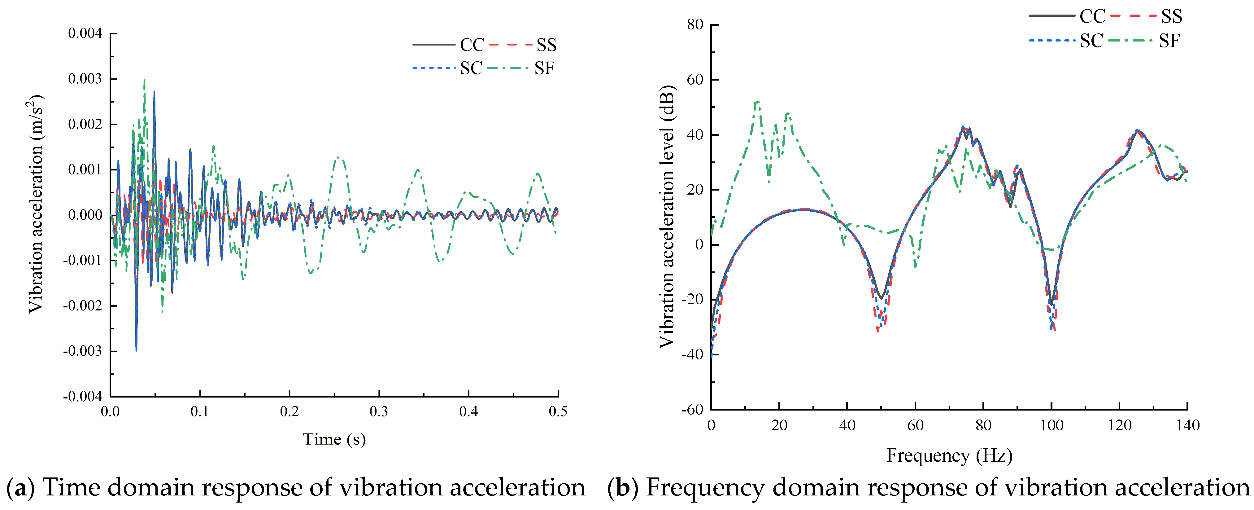
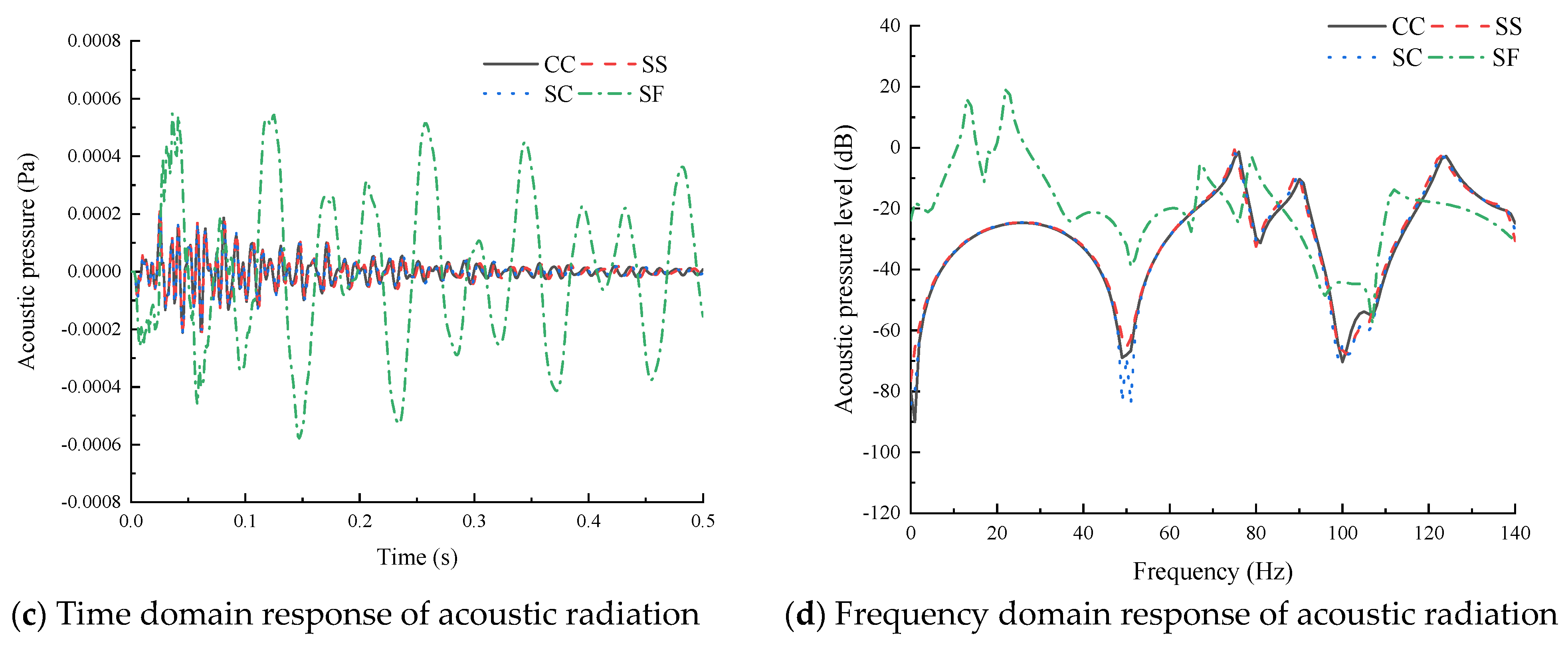
• Changes in structural parameters such as boundary conditions and semi-vertex angle had a great effect on the vibro-acoustic response. As the stiffness of the boundary conditions decreased, the natural frequency moved to the left. When the length and thickness were fixed, the natural frequency of the structure decreased with an increase in the semi-vertex angle; the amplitude of the vibro-acoustic response increased, and the peak frequency of the forced vibration response moved to the left.
• The characteristic line spectrum of the forced vibration response and acoustic radiation of the conical shell under an impulse load and random load excitation was caused by the natural frequency of the structure and the peak value of the excitation load. At the natural frequency of the structure, the small excitation load may also cause a strong characteristic line spectrum.

References

1. Caresta, M.; Kessissoglou, N.; Tso, Y. Low frequency structural and acoustic responses of a submarine hull. Acoust. Aust. 2008, 36, 47–52. [Google Scholar]
2. Caresta, M.; Kessissoglou, N.J. Acoustic signature of a submarine hull under harmonic excitation. Appl. Acoust. 2010, 71, 17–31. [Google Scholar] [CrossRef]
3. Lam, K.; Li, H.; Ng, T.; Chua, C. Generalized differential quadrature method for the free vibration of truncated conical panels. J. Sound Vib. 2002, 251, 329–348. [Google Scholar] [CrossRef]
4. Guo, C.; Liu, T.; Bin, Q.; Wang, Q.; Wang, A. Free vibration analysis of coupled structures of laminated composite conical, cylindrical and spherical shells based on the spectral-Tchebychev technique. Compos. Struct. 2022, 281, 114965. [Google Scholar] [CrossRef]
5. Chen, M.; Xie, K.; Jia, W.; Xu, K. Free and forced vibration of ring-stiffened conical–cylindrical shells with arbitrary boundary conditions. Ocean Eng. 2015, 108, 241–256. [Google Scholar] [CrossRef]
6. Xie, K.; Chen, M.; Dong, W.; Li, W. A unified semi-analytical method for vibration analysis of shells of revolution stiffened by rings with T cross-section. Thin-Walled Struct. 2019, 139, 412–431. [Google Scholar] [CrossRef]
7. Caresta, M.; Kessissoglou, N.J. Free vibrational characteristics of isotropic coupled cylindrical–conical shells. J. Sound Vib. 2010, 329, 733–751. [Google Scholar] [CrossRef]
8. Ye, T.; Jin, G.; Chen, Y.; Ma, X.; Su, Z. Free vibration analysis of laminated composite shallow shells with general elastic boundaries. Compos. Struct. 2013, 106, 470–490. [Google Scholar] [CrossRef]
9. Qu, Y.; Hua, H.; Meng, G. A domain decomposition approach for vibration analysis of isotropic and composite cylindrical shells with arbitrary boundaries. Compos. Struct. 2013, 95, 307–321. [Google Scholar] [CrossRef]
10. Su, Z.; Jin, G.; Shi, S.; Ye, T.; Jia, X. A unified solution for vibration analysis of functionally graded cylindrical, conical shells and annular plates with general boundary conditions. Int. J. Mech. Sci. 2014, 80, 62–80. [Google Scholar] [CrossRef]
11. Tong, B.; Li, Y.; Zhu, X.; Zhang, Y. Three-dimensional vibration analysis of arbitrary angle-ply laminated cylindrical shells using differential quadrature method. Appl. Acoust. 2019, 146, 390–397. [Google Scholar] [CrossRef]
12. Jafari, A.; Khalili, S.; Azarafza, R. Transient dynamic response of composite circular cylindrical shells under radial impulse load and axial compressive loads. Thin-Walled Struct. 2005, 43, 1763–1786. [Google Scholar] [CrossRef]
13. Forouzesh, F.; Jafari, A.A. Nonlinear Forced vibration of pseudoelastic shape memory alloy cylindrical shell subjected to the time and space dependant internal pressure. Modares Mech. Eng. 2015, 15, 1–12. [Google Scholar]
14. Li, H.; Pang, F.; Miao, X.; Du, Y.; Tian, H. A semi-analytical method for vibration analysis of stepped doubly-curved shells of revolution with arbitrary boundary conditions. Thin-Walled Struct. 2018, 129, 125–144. [Google Scholar] [CrossRef]
15. Li, H.; Pang, F.; Miao, X.; Li, Y. Jacobi–Ritz method for free vibration analysis of uniform and stepped circular cylindrical shells with arbitrary boundary conditions: A unified formulation. Comput. Math. Appl. 2019, 77, 427–440. [Google Scholar] [CrossRef]
16. Pang, F.; Li, H.; Wang, X.; Miao, X.; Li, S. A semi analytical method for the free vibration of doubly-curved shells of revolution. Comput. Math. Appl. 2018, 75, 3249–3268. [Google Scholar] [CrossRef]
17. Qu, Y.; Meng, G. Prediction of acoustic radiation from functionally graded shells of revolution in light and heavy fluids. J. Sound Vib. 2016, 376, 112–130. [Google Scholar] [CrossRef]
18. Qu, Y.; Meng, G. Vibro-acoustic analysis of multilayered shells of revolution based on a general higher-order shear deformable zig-zag theory. Compos. Struct. 2015, 134, 689–707. [Google Scholar] [CrossRef]
19. Zhong, R.; Hu, S.; Liu, X.; Qin, B.; Wang, Q.; Shuai, C. Vibro-acoustic analysis of a circumferentially coupled composite laminated annular plate backed by double cylindrical acoustic cavities. Ocean Eng. 2022, 257, 111584. [Google Scholar] [CrossRef]
20. Zhong, R.; Guan, X.; Wang, Q.; Qin, B.; Shuai, C. Prediction of acoustic radiation from elliptical caps of revolution by using a semi-analytic method. J. Braz. Soc. Mech. Sci. Eng. 2021, 43, 383. [Google Scholar] [CrossRef]
21. Sharma, N.; Mahapatra, T.R.; Panda, S.K. Numerical analysis of acoustic radiation properties of laminated composite flat panel in thermal environment: A higher-order finite-boundary element approach. Proc. Inst. Mech. Eng. Part C J. Mech. Eng. Sci. 2018, 232, 3235–3249. [Google Scholar] [CrossRef]
22. Kumar, B.R.; Ganesan, N.; Sethuraman, R. Vibro-acoustic analysis of functionally graded elliptic disc under thermal environ-ment. Mech. Adv. Mater. Struct. 2009, 16, 160–172. [Google Scholar] [CrossRef]
23. Gao, C.; Zhang, H.; Li, H.; Pang, F.; Wang, H. Numerical and experimental investigation of vibro-acoustic characteristics of a submerged stiffened cylindrical shell excited by a mechanical force. Ocean Eng. 2022, 249, 110913. [Google Scholar] [CrossRef]
24. Pang, F.; Tang, Y.; Qin, Y.; Zheng, J.; Hui, D.; Li, H. Analysis of acoustic radiation characteristic of laminated paraboloidal shell based on Jacobi-Ritz-spectral BEM. Ocean Eng. 2023, 280, 114686. [Google Scholar] [CrossRef]
25. Xie, K.; Chen, M. A semi-analytic model for vibro-acoustic analysis of functionally graded shells of revolution. Thin-Walled Struct. 2022, 173, 108949. [Google Scholar] [CrossRef]
26. Xie, K.; Chen, M.; Zhang, L.; Li, W.; Dong, W. A unified semi-analytic method for vibro-acoustic analysis of submerged shells of revolution. Ocean Eng. 2019, 189, 106345. [Google Scholar] [CrossRef]
27. Li, Z.; Wang, Q.; Zhong, R.; Qin, B.; Shao, W. Vibro-acoustic analysis of laminated composite cylindrical and conical shells using meshfree method. Eng. Anal. Bound. Elements 2023, 152, 789–807. [Google Scholar] [CrossRef]
28. Jin, G.; Ma, X.; Wang, W.; Liu, Z. An energy-based formulation for vibro-acoustic analysis of submerged submarine hull struc-tures. Ocean. Eng. 2018, 164, 402–413. [Google Scholar] [CrossRef]
29. Chen, M.; Zhang, C.; Tao, X.; Deng, N. Structural and acoustic responses of a submerged stiffened conical shell. Shock Vib. 2014, 2014, 954253. [Google Scholar] [CrossRef]
30. Wang, X.; Wu, W.; Yao, X. Structural and acoustic response of a finite stiffened conical shell. Acta Mech. Solida Sin. 2015, 28, 200–209. [Google Scholar] [CrossRef]
31. Wang, X.-Z.; Jiang, Q.-Z.; Xiong, Y.-P.; Gu, X. Experimental studies on the vibro-acoustic behavior of a stiffened submerged conical-cylindrical shell subjected to force and acoustic excitation. J. Low Freq. Noise, Vib. Act. Control 2020, 39, 280–296. [Google Scholar] [CrossRef]
32. Qu, Y.; Zhang, W.; Peng, Z.; Meng, G. Time-domain structural-acoustic analysis of composite plates subjected to moving dynamic loads. Compos. Struct. 2019, 208, 574–584. [Google Scholar] [CrossRef]
33. Zuo, Y.; Yang, D.; Zhuang, Y. Broadband transient vibro-acoustic prediction and control for the underwater vehicle power cabin with metamaterial components. Ocean Eng. 2024, 298, 117121. [Google Scholar] [CrossRef]
34. Gao, C.; Xu, J.; Pang, F.; Li, H.; Wang, K. Modeling and experiments on the vibro-acoustic analysis of ring stiffened cylindrical shells with internal bulkheads: A comparative study. Eng. Anal. Bound. Elements 2024, 162, 239–257. [Google Scholar] [CrossRef]
35. Gao, C.; Pang, F.; Li, H.; Huang, X.; Liang, R. Prediction of vibro-acoustic response of ring stiffened cylindrical shells by using a semi-analytical method. Thin-Walled Struct. 2024, 200, 111930. [Google Scholar] [CrossRef]
36. Wang, Q.; Shi, D.; Liang, Q.; Pang, F. Free vibrations of composite laminated doubly-curved shells and panels of revolution with general elastic restraints. Appl. Math. Model. 2017, 46, 227–262. [Google Scholar] [CrossRef]
37. Gao, C.; Pang, F.; Cui, J.; Li, H.; Zhang, M.; Du, Y. Free and forced vibration analysis of uniform and stepped combined coni-cal-cylindrical-spherical shells: A unified formulation. Ocean. Eng. 2022, 260, 111842. [Google Scholar] [CrossRef]
Figure 1. Calculation model of conical shell.
Acoustics 06 00028 g001
Figure 2. Coordinate system of external acoustic radiation from conical shell.
Acoustics 06 00028 g002
Figure 3. Forced vibration excitation load.
Acoustics 06 00028 g003
Figure 4. Natural frequency comparison of conical shell.
Acoustics 06 00028 g004
Figure 5. Absolute percentage errors of natural frequency under different Jacobi parameters.
Acoustics 06 00028 g005
Figure 6. Acoustic pressure level under different truncation numbers of sound pressure function.
Acoustics 06 00028 g006
Figure 7. The vibro-acoustic responses compared with FEM/BEM.
Acoustics 06 00028 g007
Figure 8. Response curve under different boundary conditions.
Acoustics 06 00028 g008aAcoustics 06 00028 g008b
Figure 9. Vibro-acoustic characteristic curves under different semi-vertex angles.
Acoustics 06 00028 g009
Figure 10. Vibro-acoustic characteristic curves under different excitation loads.
Acoustics 06 00028 g010
Figure 11. Acoustic radiation directivity patterns with different circumferential distances. (a) Acoustic radiation directivity patterns in time domain at 0.5 s. (b) Acoustic radiation directivity patterns in time domain at 0.7s. (c) Acoustic radiation directivity patterns in frequency domain at 75 Hz. (d) Acoustic radiation directivity patterns in frequency domain at 125 Hz.
Acoustics 06 00028 g011aAcoustics 06 00028 g011b
Figure 12. Amplitude curve of random excitation load.
Acoustics 06 00028 g012
Figure 13. Vibro-acoustic characteristic curves of random excitation load.
Acoustics 06 00028 g013