Article

Identification of the Aeroacoustic Emission Source Regions Within a Ceiling Swirl Diffuser

Institute for Energy Efficient Buildings and Indoor Climate, E.ON Energy Research Center, RWTH Aachen University, 52074 Aachen, Germany
*
Author to whom correspondence should be addressed.
Acoustics 2025, 7(1), 9; https://doi.org/10.3390/acoustics7010009
Submission received: 4 November 2024 / Revised: 16 January 2025 / Accepted: 18 February 2025 / Published: 24 February 2025

Abstract

:
The acoustic emissions of ventilation systems and their subcomponents contribute to the perceived overall comfort in indoor environments and are, therefore, the subject of research. In contrast to fans, there is little research on the aeroacoustic properties of air diffusers (often referred to as outlets). This study investigates a commercially available ceiling swirl diffuser. Using a hybrid approach, a detailed three-dimensional large-eddy simulation is coupled with a perturbed wave equation to capture the aeroacoustic processes within the diffuser. The flow model is validated for the investigated operating point of 470 m3/h using laser-optical and acoustic measurements. To identify the noise sources, the acoustic pressure is sampled with various receivers and on cut sections to evaluate the cross-power spectral density, and the sound-pressure level distribution on cut sections is evaluated. It is found that the plenum attenuates the noise near its acoustic eigenmodes and thus dominates other noise sources by several orders of magnitude. By implementing the plenum walls as sound-absorbing, the overall sound-pressure level is predicted to decrease by nearly 10 dB/Hz. Other relevant geometric features are the mounting beam and the guide elements, which are responsible for flow-borne noise emissions near 698 Hz and 2699 Hz, respectively.

Graphical Abstract

1. Introduction

When providing a productive indoor environment, acoustic comfort is one key factor in rating the indoor environmental quality. As an increasing number of buildings are equipped with mechanical ventilation systems, their acoustic emission is gaining importance. Ventilation systems consist of components such as fans, control devices, ducts, and air diffusers (also referred to as outlets). Air diffusers represent the last component of the ventilation system and are responsible for distributing the supplied air into the room. While the main goal is an even air distribution in the room without causing discomfort, they are also subject to visual design requirements. In addition to providing fresh, uncontaminated air into the room, ventilation systems provide heating and cooling using higher or lower temperatures for the supply air compared to the room temperature. To provide a certain thermal power, both the volume flow rate and the temperature difference need control. As the volume flow rate is strongly coupled to the acoustic emissions, which are subject to regulations, the volume flow rate is limited to a maximum value [1]. Reducing the acoustic emissions enables a higher volume flow rate, consequently allowing for lower temperature differences. The lower temperature differences benefit the operation of heat pumps or chillers. Typical ventilation systems feature multiple sound absorbers inside either the air handling units (AHU) themselves or throughout the duct network. These sound absorbers can effectively reduce the sound emission from both the AHU and the ducting at the cost of increased pressure losses. Therefore, the implementation of sound absorbers might not always be feasible. Air diffusers often are not yet subject to dedicated acoustic treatment.
Winkelmann et al. [2] conducted a subject study where they presented various sound samples of different air diffusers. They found that mainly the loudness and, consequently, the volume flow are responsible for the acoustic comfort. In two studies, Stürenburg et al. [3,4] presented experiments where they assessed the sound emissions of different air diffusers. They found that most of the significant characteristics of the emitted noise are contained within a frequency range of up to 5000 Hz. Due to the low overall emission levels, the proper resolution of the acoustic signals was challenging. The identification of the responsible emission sources within the investigated diffuser flows was not attempted.
In the case of air diffusers, where most of the noise source regions are difficult to investigate with experimental methods, simulation models make it possible to investigate the aeroacoustic behavior properly. Due to the relatively low flow velocity present in the field of indoor ventilation, the flow can be assumed to be incompressible. To resolve acoustic pressure fluctuations, hybrid approaches have been developed and proven to accurately predict the emerging acoustic emission of incompressible flows. Prominent approaches are based on the Ffowcs–Williams Hawkings (FW-H) approach [5], the Acoustic Perturbed Equations (APE) [6] and different perturbed wave equations [7,8,9,10].
Although this article does not investigate the aeroacoustics of fans, some selected studies (see [11,12,13,14,15,16,17,18,19,20,21]) are summarized here, as considerably more research is conducted in that field compared to air diffusers. Significant improvements to their emissions were achieved in the past by treating the leading and/or trailing edges of the blades. Several studies found that the periodic interaction between the individual blades and their wake flow structures is one main contributor to the emitted noise. The periodic interactions produce tonal components at harmonics of the so-called “blade passing frequency” (BPF). Suitable modifications of either the flow field or the leading edges can reduce the acoustic emissions significantly, although this might come at the cost of reduced aerodynamic efficiency [11,12,13]. These studies were either conducted experimentally [11,12,13,14,15,16] or numerically, where different methods of Computational Aeroacoustics (CAA) were applied. They either conducted so-called Direct Noise Computations (DNC) [17,18] or applied hybrid approaches such as the FW-H analogy [20] or perturbed wave equations [19]. Success was also achieved by conducting steady-state flow simulations [20,21]. However, the steady-state flow results did not allow a frequency-resolved evaluation of the sources.. In the case of fans, a reduction of noise emissions is mainly achieved by reducing the sound-pressure level of the tonal components at the BPF harmonics.
Within the field of automotive applications, control devices such as flaps and complex duct networks were investigated. Therefore, the studies in this field are more relevant to the topic of this paper. To some extent, the same numerical methods as for fans are applicable. Perot et al. [22] conducted a DNC of an automotive ventilation duct system and found certain duct modes that were acoustically excited. By applying broadband source models (see [23,24]) based on steady-state simulations, Khondge et al. [25] and Mohamud and Johnson [26] were able to locate the main sound emission regions within different duct components and improve the corresponding designs. In two studies, Ravichandran et al. [27,28] investigated a generic air diffuser by applying the hybrid approach based on the Acoustic Perturbed Equations (APE) derived by Ewert and Kreuzinger [29]. They found a certain eigenmode of the investigated duct geometry to be mainly responsible for the noise emission. Fenini [30] conducted an extensive study of an orifice and its aeroacoustic emissions by coupling another hybrid APE formulation derived by Bechara et al. [31] with steady-state simulations. Although they can adequately predict the acoustic pressure at a certain distance from the investigated device, his work lacks near-field accuracy. A whole automotive ventilation system was investigated by Tautz [19] using a perturbed wave equation approach. He identified the fan and the diffusers as the main noise sources. When investigating air diffusers, the FW-H approach is not applicable as it relies on the definition of suitable control surfaces that must not be penetrated by the flow itself. Typical air diffusers in the scope of building-related ventilation systems differ strongly from their automotive counterparts, yet the flow velocity is in roughly the same range. They usually feature large plenums that attenuate and alter the sound characteristics.
Saarinen and Koskela [32] and Saarinen and Mustakallio [33] investigated two exhaust valves often used in the scope of smaller ventilation systems such as residential buildings. Two studies investigated a slot diffuser [34,35]. By conducting steady-state simulations coupled to broadband noise source levels and transient simulations, they were able to locate several edges that are responsible for noise emission. However, geometric modifications based on steady-state results were not sufficient to reduce the aeroacoustic emissions. In an earlier study, the authors already investigated the emissions of a ceiling swirl diffuser [36] and identified the acoustic eigenmodes of the plenum as strong contributors to the emissions. Although it was possible to predict the mean flow-field properly, the agreement of the predicted aeroacoustic emissions to the measurements was poor. The experimental setup did not allow for a proper resolution of the acoustic signals due to the high background noise of the air supply. Furthermore, their flow model was not able to achieve turbulence levels that were close to the measurements.
This study aims to present a methodology utilizing numerical flow simulations coupled with a hybrid aeroacoustic approach to aid in the early-stage design of air diffusers. The conducted experiments include aerodynamic, laser-optical and acoustic measurements. These are used to validate the numerical flow model, which features an improved turbulence generation compared to the previous study [36]. The evaluation of the acoustic emissions is made by implementing several receivers where the acoustic pressure is sampled. The precise identification and localization of relevant noise source regions are made possible by spatially resolving the acoustic pressure on cut sections in addition to the receiver locations. By further filtering the spatially resolved acoustic pressure to certain frequency bands, the contribution of certain geometric features to the overall emitted spectrum is derived.

2. Methods

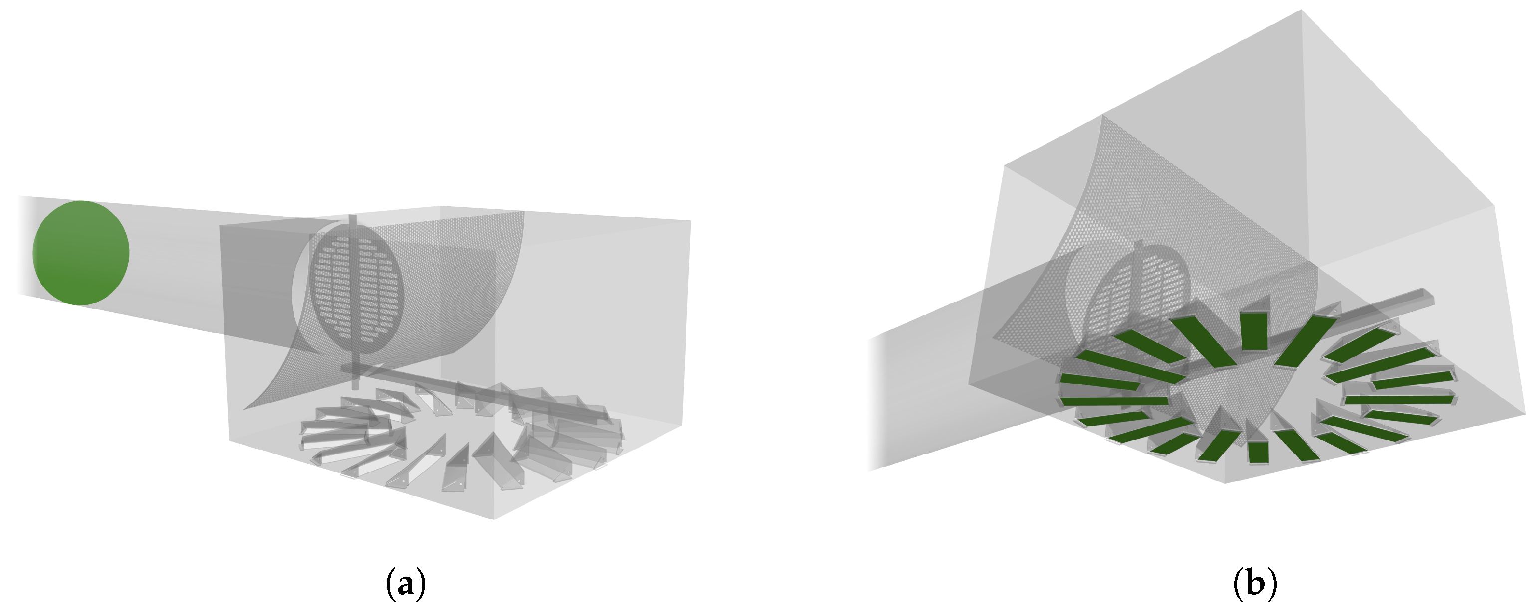
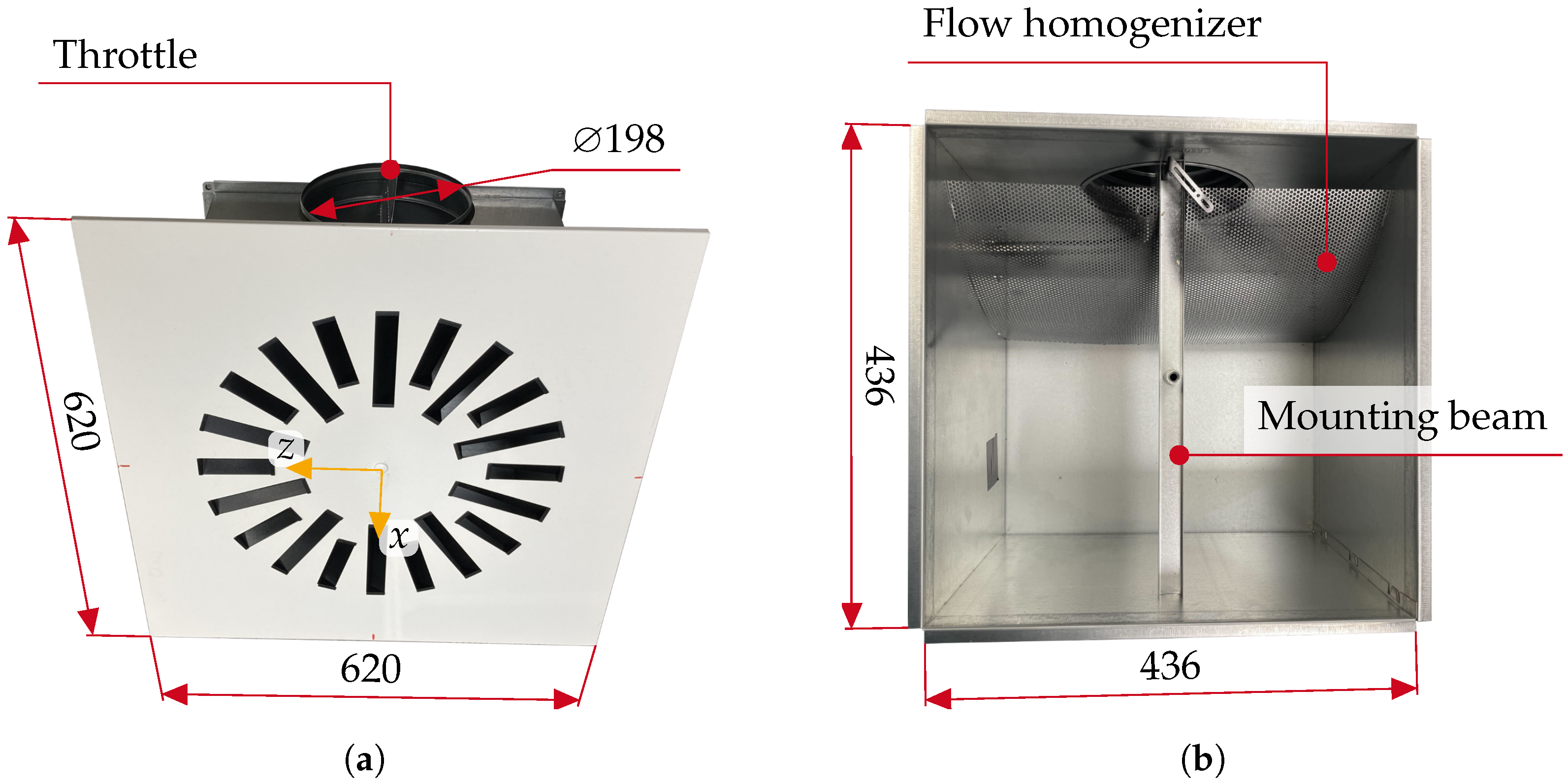
2.1. Investigated Swirl Diffuser

This study investigates a commercial swirl diffuser, as shown in Figure 1. The picture of the total assembly Figure 1a features the coordinate system used in this study. It consists of a cuboid plenum featuring inner dimensions of 0.436 × 0.436 × 0.2848 m and a diffuser plate. A flow homogenizer and a mounting beam are located inside the plenum, as shown in Figure 1b. The mounting beam is used to attach the diffuser plate to the plenum. The air is fed into the plenum through a circular duct (DDuct = 198 mm) located on one side of the plenum. An additional throttle is installed inside the connecting duct to adapt the volume flow rate in a multi-diffuser ventilation system. In the scope of this study, the throttle is fully opened and, therefore, parallel to the flow direction. Downstream of the duct, a perforated hole plate serves as a flow homogenizer. The diffuser plate features 20 guide elements, alternating between a long and a short version.

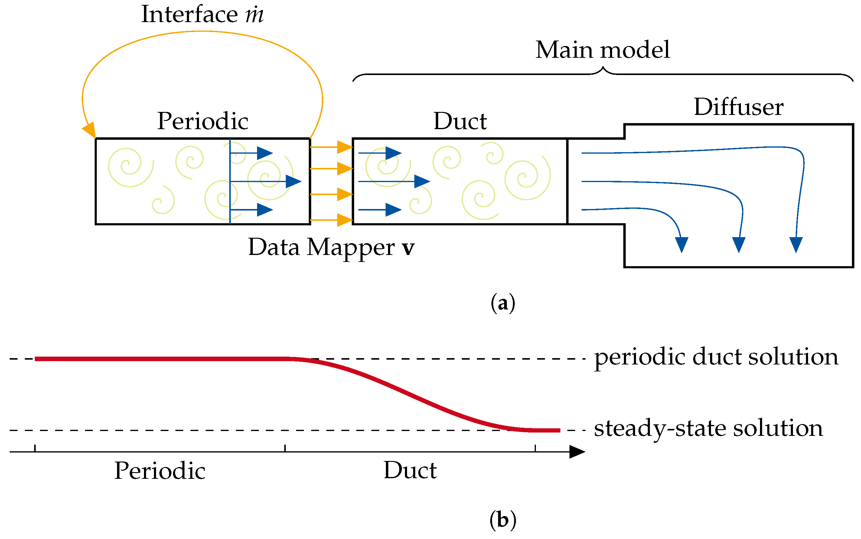
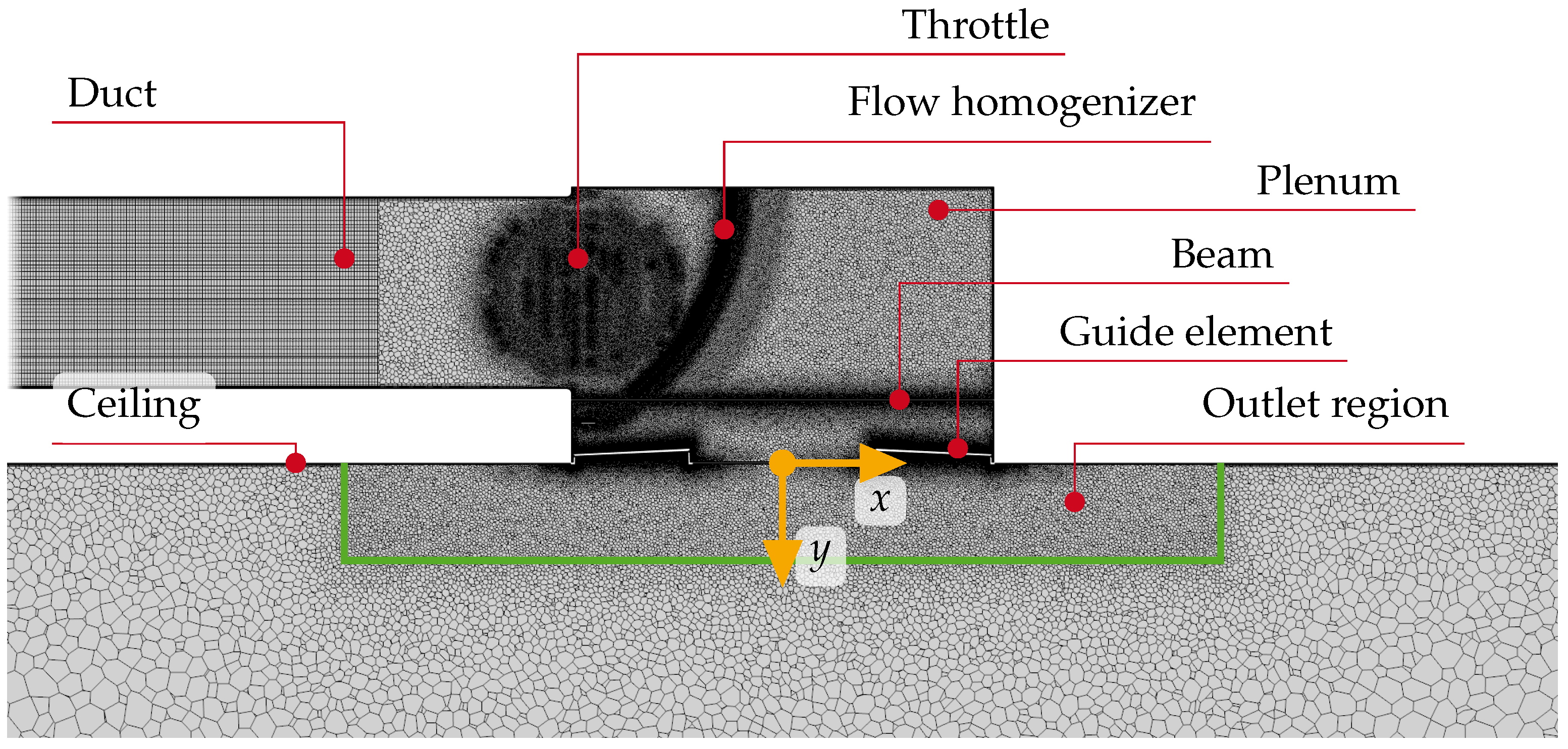
2.2. Numerical Model

The transient, numerical 3D flow simulations presented in this study are performed using the commercial software STAR-CCM+ 18.04.008 distributed by Siemens [37]. The diffuser’s geometry is modified slightly to enable the successful generation of a suitable computational mesh. The main modifications include the closing of small gaps between the guide elements and the diffuser plate and neglecting all connecting elements like nuts or screws. The diffuser is connected to a simplified room with the dimensions of 4 × 4 × 1.5 m. Based on the experimentally observed flow pattern, these dimensions are sufficient to allow the flow to develop properly.
The airflow is modeled as an incompressible fluid and computed by solving the conservation equations for mass Equation (1) and momentum Equation (2) using the SIMPLE algorithm.
ρ t + · ρ v = 0
ρ v t + · ρ vv = · T + ρ b
The choice of the turbulence models and the description of the hybrid CAA approach is described later in this section. The corresponding properties of the air are summarized in Table 1.
As the inflow turbulence is of great importance to the aeroacoustic behavior of the diffuser (see [36]), a periodic boundary condition is implemented. The periodic boundary condition enables the specification of a fully developed, spatially and time-resolved flow field as the boundary condition for the main flow model. Based on manufacturer data, the operating point at 470 m3/h is chosen, as it is in the middle of the design range of this particular diffuser. This volume flow rate corresponds to a mass flow rate m ˙ of 0.1572 kg/s, which is set as the target value for the periodic interface of the duct segment upstream of the actual flow model. The periodic interface employs an internal control strategy that maintains the flow rate by adapting the pressure on the downstream interface boundary. This approach makes it possible to pass on a detailed calibration of synthetic turbulence generation models (see [38,39,40,41]) to the presented flow problem.
The periodic duct segment is initialized and then coupled to the main simulation model. The computed velocity distribution v on the downstream outlet surface of the periodic duct segment is mapped onto an inlet velocity boundary condition on the upstream inlet surface of the duct segment. The mapping process is carried out every time step, effectively one-way coupling the periodic duct to the main model. The periodic duct segment is initialized by pre-computing it in an isolated setup for 5 s with a time step of 1 × 10⁻⁴ s. This setup is referred to as the “periodic duct model” hereafter and represents a separate flow model that is solved prior to the main transient flow model. Considering the average flow velocity within the periodic duct and its length, this time frame corresponds to a virtual duct length of 14.9 m that is covered by the flow inside the periodic duct. This is long enough to allow the turbulent kinetic energy k to converge to a sufficiently stable level. The required computational resources of the periodic model are negligible compared to the overall cost and enable a proper initialization and definition of the flow problem.
The transient flow model is initialized by interpolating the steady-state solution of the combined model (periodic and main model) with the pre-computed periodic duct solution. The steady-state calculation utilizes the same framework shown in Figure 2a, where the mapping occurs at every iteration. After both the steady-state solution and the periodic duct solution are computed, the transient periodic duct solution is duplicated into the main model’s duct segment. This leads to both the periodic duct solution and the respective steady-state solution being present in the main model’s duct segment. Inside the main model’s duct segment, an interpolated solution is then calculated using a sine function, as shown in Figure 2b. Therefore, the initial solution for the main transient calculation consists of the periodic duct, the interpolated duct, and the main model’s diffuser solution. The same mesh is applied in the duct and periodic parts of the model to reduce interpolation errors, when the periodic duct solution is copied into the duct segment.
To properly resolve the relevant aeroacoustic phenomena, the technically relevant frequency range of 100–5000 Hz is defined, which the coupled acoustic-flow model should capture with sufficient resolution. The lower and upper limit is called the cut-on frequency fcut-on and cut-off frequency fcut-off, respectively. Experimental results show that most of the aeroacoustic characteristics can be obtained by investigating this frequency range [3,4]. Limiting the resolved frequency to this range saves on computational costs. Furthermore, the selected frequency range matches well with the A-rating of sound, where the sensitivity of the human ear is approximated [42]. Based on the “Nyquist-Shannon”-criterion, the necessary sampling rate fs to capture such a signal is defined according to Equation (3) [43,44,45,46].
f s > 2 · f signal
Furthermore, an oversampling factor of k oversampling = 10 is imposed to compensate for noise in the resulting signals [47]. The oversampling ensures a valid evaluation of frequencies up to 5000 Hz. Towards higher frequencies, the influence of signal noise increases, yet the oversampling reduces these effects to some extent. The necessary timestep Δ t of the simulation is calculated by extending the definition from Equation (3) to Equation (4). With a similar approach, the necessary sampling time T s to capture the low-frequency components is estimated according to Equation (5).
Δ t 1 f s = 1 k oversampling · 2 · f cut - off = 1 × 10 5   s
T s 2 f cut - on · k oversampling = 0.2   s
This time step size of 1 × 10⁻⁵ s is used throughout the entire transient simulation and is one magnitude smaller than the time step size used for the periodic duct model. In total, a time frame of 0.4 s is computed in the simulation, of which only the last 0.2 s are evaluated. The total simulation time is based on the turbulent behavior of the flow, which is presented in the Section 3.
The wavelength λ of a sound wave moving with the speed of sound c is directly coupled to its frequency f according to Equation (6). The necessary mesh resolution Δ is approximated based on the expected wavelength λ of a wave oscillating at the cut-off frequency. This leads to the expression according to Equation (7).
λ = c f
λ Δ < c f cut - off
As shown by Zingg et al. [48], a certain number of points per wavelength (short: PPW) is necessary to capture acoustic waves and their propagation through space properly. Following the recommendations of Zingg et al. [48], a value of PPW = 20 is chosen, from which an approximation of the upper limit for the mesh resolution in the region of interest is derived according to Equation (8) [48].
Δ < c PPW · f cut - off = 3.4 × 10 3   m
A maximum mesh resolution of Δ = 3 mm is consequently imposed within the whole region of interest.
All wall boundaries employ prism layer cells to resolve the boundary layer. The boundary layer is resolved by five prism layers, with a constant stretching factor of 1.5. Except for the flow homogenizer, the total thickness of all prism layers is within the range of 0.9–1.5 mm. The finer resolution is employed on the guide elements and the diffuser plate. On the flow homogenizer, the total thickness of the prism layer is further reduced to 0.45–1.2 mm, where the holes feature the finest resolution. These settings yield a dimensionless wall distance of up to y + < 6 near sharp edges. All major flat surfaces and the duct walls feature values of y + < 1 .
Figure 3 shows a section of the computational mesh on the x-y-section at z = 0 mm. The region of interest comprises the inflow duct, the diffuser itself, and the outlet region marked by the green line. As can be seen, the mesh is locally refined down to 0.125 mm to capture geometric features like small radii or the holes of the flow homogenizer. Due to the available memory during the meshing process, the mesh can only be refined locally. In total, the mesh based on these design criteria consists of roughly 126,453,800 cells.
Usually, the computational mesh is designed with the aid of a mesh independence study as proposed by Celik et al. [49] and Roache [50]. However, due to multiple local refinements to capture the areas of high flow activity, the application of their approach is not fully possible in the presented case. To investigate the mesh dependency of the results, the mesh resolution of only the local refinements is changed instead of scaling the overall mesh resolution. Regarding the limited computational resources available for this study, mesh dependency is investigated using steady-state RANS simulation by analyzing the pressure loss and the TKE on the diffuser outlet section. The TKE is important as the turbulence behavior is expected to be essential for the acoustic processes that are investigated in this study.
In total, four additional meshes are generated that feature gradually coarser mesh resolutions of the local refinements. In addition to the mesh resolution, the volumetric and surface growth rates are increased from 1.05 to 1.1 as the mesh becomes coarser. As shown in Figure 4, the pressure loss across the diffuser is not dependent on the mesh size in the investigated range. However, the TKE on the diffuser outlet section features a clear asymptotic trend towards the larger mesh and, thus, smaller mesh resolutions. Although the mesh independence study is performed using steady-state RANS calculations, the requirements for the mesh resolution imposed by LES calculations are expected to be even stricter. Therefore, the finest mesh featuring the largest number of cells is selected for this study. Any further computational mesh refinement would increase the computing costs to an unreasonable level.
By estimating the maximum flow velocity and assuming the minimal mesh resolution, the CFL-number is evaluated according to Equation (9) [51].
CFL = | v cell | Δ t Δ x cell = 10   m / s · 1   ×   10 5   s 0.125   ×   10 3   m = 0.8 1
Other authors achieved accurate results by using less restrictive values for the PPW-criterion or the simulation timestep [10,19,22,29,30].
The resulting mesh cut-off frequency is shown on a x-y-section and along the y-axis in Figure 5. Here, the mesh resolution in Equation (8) is approximated using the cubic root of the cell volume ( Δ = V cell 3 ). Within the plenum and the outlet region, the cut-off frequency satisfies the required value of 5000 Hz. Upon increasing distance from the diffuser, the cut-off frequency rapidly declines towards smaller values. At y = 0.3 m it features a value near 1000 Hz whereas in the far field (y > 0.7 m) the value drops below 500 Hz. This showcases the disparity of scales often associated with aeroacoustic problems. The flow requires a fine mesh to resolve the flow structures that generate noise. Additionally, the sound waves require a certain mesh resolution for proper propagation. Due to the large geometry of the investigated diffuser, a large number of cells is already required to properly resolve the diffuser flow. An extension of the region with proper mesh resolution to larger distances to also propagate the sound waves far away from the diffuser would improve the respective mesh cut-off frequency but significantly increase the computational cost.
For the steady-state precursor simulation and mesh independence study, the turbulence is modeled utilizing the “k- ε Realizable Two-Layer”-model following the “Reynolds-Averaged Navier–Stokes” (RANS) approach [37,52,53]. One key feature of the diffuser flow is the attachment of the flow to the ceiling. This feature was not captured when using the k-ω-SST model [54]. Since the steady-state model is not evaluated in detail, a detailed analysis of possible reasons is not conducted. In the case of the transient simulation, also including the periodic initialization submodel, a large-eddy simulation (LES) with the WALE subgrid-scale model [55] is performed.
The generation and propagation of the aeroacoustic emissions are modeled with the wLPCE (“wave Linearized Perturbed Compressible Equation”) approach proposed by Piepiorka and von Estorff [10], which solves for the acoustic potential Φ. They derived their wave equation from the works of Seo and Moon [7,8] and Hüppe [9]. It is a hybrid approach, where the sound generation is derived from the incompressible, hydrodynamic pressure fluctuations. This effectively decouples hydrodynamic pressure fluctuations from the acoustic pressure, allowing for a sampling of the acoustic pressure in regions with strong flow activity. Within STAR-CCM+ the formulation is extended by an additional damping term τ and a source-term S Φ according to Equation (10) [37]. The user-defined source-term S Φ is not used in this study and therefore set to zero.
D 2 Φ D t 2 c 2 Δ Φ + τ Φ t 1 ρ ¯ Φ · p ic = 1 ρ ¯ D p ic D t + S Φ
The damping term τ is defined according to Equation (11) using the speed of sound and the respective cell volume V cell where the damping is evaluated.
τ = b d V cell 3 π c
Damping is used in this study to prevent the generation of aeroacoustic sources in regions with a coarse computational grid by defining the damping coefficient b d , as shown in Figure 6. The walls of the simplified room are defined as pressure outlets with sound-absorbing behavior. The room ceiling the diffuser is attached to is modeled as a wall with sound-reflecting behavior. The plenum walls are assumed to be perfectly stiff walls and, therefore, sound-reflecting as well.
The simulation is divided into four phases. During the first phase, the steady-state solution and the periodic duct solution are computed. They are combined and interpolated into the transient initial solution. During the second phase, the transient solution is computed for 0.05 s employing a 2nd-order accurate bounded central scheme. The second phase allows the flow to further develop from the interpolated initial solution generated in the first phase. At the start of the third phase, which covers the time frame between 0.05 s < t ≤ 0.1 s, the convection scheme is switched to a more accurate 3rd-order MUSCL/CD scheme and the aeroacoustic computation is enabled. During the third phase, the aeroacoustic propagation and the flow further develop. The final, fourth phase covers the acoustic sampling time frame of 0.3 s between 0.1 s < t ≤ 0.4 s, of which only the interval of the last 0.2 s is used for evaluation. To cut computational cost without decreasing the accuracy, individual convergence criteria for the non-normalized residuals are implemented. They are set up to trigger between five and ten inner iterations if the momentum residuals decrease below 2 × 10⁻⁸ and the continuity residual decreases below 2 × 10⁻¹⁰. These criteria ensure that convergence is achieved in each time step.

2.3. Evaluation of the Flow Model

The velocity field is sampled on the exit cross-section from the periodic duct segment (“Periodic”) and in the outlet section of the diffuser plate (“Diffuser”). From these data, the average flow velocity |v| and turbulent kinetic energy (TKE) k are computed on both sections to evaluate the development of the flow. The evaluation of the TKE is described in more detail in Appendix A.
The surface averaged TKE is evaluated at increments of 0.01 s with a sample window of 0.05 s or N = 5000 timesteps on both evaluation sections. This aids in the decision on when the flow field has sufficiently developed to quasi-stationary behavior in order to begin the acoustic sampling.
As the main goal of the flow simulation is the prediction of the acoustic emissions, several receiver positions are implemented at which the acoustic pressure p is sampled. The sampled signals consist of only the acoustic fluctuations since the hybrid approach decouples the hydrodynamic pressure fluctuations from the acoustic phenomena. There are receivers in each of the plenum’s corners with an additional receiver on the center of each plenum side wall. The receivers centered on the plenum walls are denoted by x , x + , y , y + , z and z + , respectively. The receivers near the plenum walls are offset by 5 mm from their corresponding surface. Within each guide element, an additional receiver is located centered in each respective outlet section. Depending on the position of the guide element, the respective receivers are denoted by their angle relative to the x-axis (e.g., 0°, 18°, …, 342°). Four receivers are located below the diffuser in an increasing distance of the plenum to up to 0.3 m while being centered in x- and z-direction, denoted by their respective distance in y-direction. The receiver in a distance of 0.1 m is located on the edge of the region of interest and, therefore, still within the region where a resolution of 5000 Hz is achieved (see Figure 5b). Using these receiver positions it is not possible to directly compare the results to the measurement setup, as the microphone is located at a significantly larger distance than the receivers. Therefore, the aim is to capture the characteristics of the acoustic emission spectrum concerning the relative decrease of the SPL and the strength of occurring peaks.
The acoustic pressure signals are used to compute the individual power spectral density (PSD) and the cross-power spectral density (CPSD) for all 741 possible receiver pairs according to Welch’s method [56]. The frequency resolution of both the PSD and the CPSD is 10 Hz and a reference value of p ref = 2 × 10 5 Pa is used for the representation in dB. Across all CPSD, an automated peak-finding is performed to extract the signal frequencies that are most dominant across all receivers. Figure 7 illustrates the application of the peak-finding to an arbitrary cross-power spectral density. The pale red line represents the actual CPSD, which, in the first step, is arithmetically averaged over a moving 1 3 -octave band yielding the dark red line. An offset of 5 dB, represented by the blue line, is defined that the CPSD must exceed in order to qualify a peak to be detected at the respective frequency. In this particular example, among others, the peaks near 800, 1300 and 2000 Hz are detected, in addition to some peaks that only marginally exceed the threshold. The number of peak occurrences is aggregated within a 1 24 -octave band as defined by DIN EN 61260 [42] across all CPSD into a histogram which is used for further analysis.
As will be discussed later, the plenum walls act as a dominant noise source without actually interacting with significant flow structures. To gain insight into the actual sources, all plenum walls are implemented as sound-absorbing in an additional flow model, resulting in an additional “absorbing” variant of the “base” model. As only the acoustic boundary conditions are changed, the flow solutions of the “base” and “absorbing” models are the same since no strong interactions between the respective acoustic and flow solutions are expected.
In addition to the receivers, as shown in Figure 8a, the three-dimensional flow domain is cut into two sections, as shown in Figure 8b. On these cut sections, the acoustic pressure is sampled, and the spatially resolved power spectral density is computed near the dominant frequencies detected by the peak-finding based on the CPSD evaluation. Limiting the evaluation to specific frequency ranges or bands enables precise localization of the respective source regions [17,19]. As the export and evaluation of the acoustic pressure on the cut sections require substantial storage capacity, this evaluation is limited to the time frame between 0.2–0.4 s of the transient calculation. Analyzing a narrow frequency band, the areas with the strongest signal within that specific frequency band are located. This information then indicates geometric features responsible for that portion of the noise emission.
When treating the plenum walls as sound-absorbing, mainly signal components that can be traced back to aerodynamically driven sources, such as turbulent vortices or fluctuating flow structures, are detected. This allows us to identify characteristic frequency bands that are worth investigating in more detail.

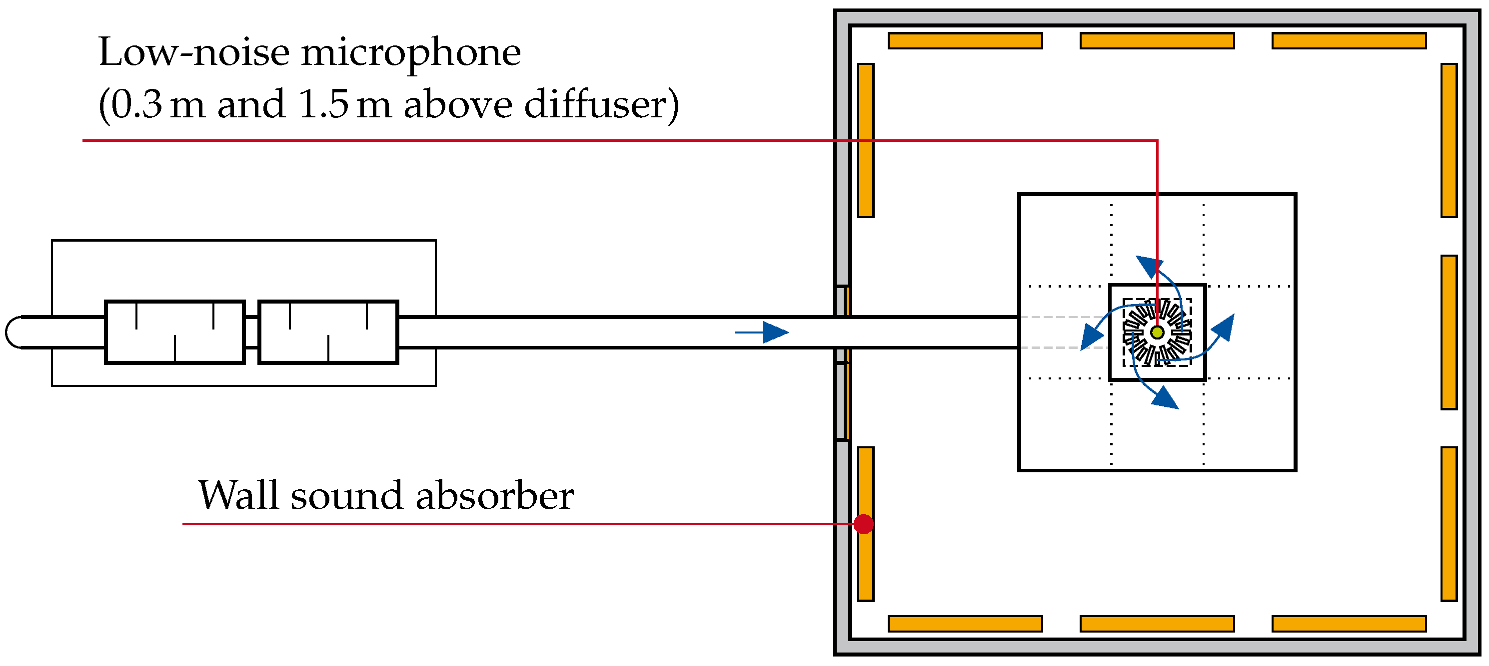
2.4. Experimental Setup

A ventilation supply unit that delivers the required flow rate with minimal acoustic emissions is utilized. The volume flow rate is calculated by measuring the pressure drop across an orifice. A schematic overview of the supply unit is shown in Figure 9. The air density of the humid air is calculated by assuming an ideal gas and utilizing the “Magnus Formula” [57]. The absolute pressure upstream of the orifice is corrected by the reference pressure differential measurement Δ p abs , ref .
The experimental setup is shown in Figure 10. A measurement chamber equipped with additional wall sound absorbers is utilized for the experimental investigations. The wall sound absorbers are placed with an offset of 0.05 m to the chamber walls to enhance the acoustic properties of the measurement chamber towards a hemi-anechoic room. The diffuser is embedded in a table-like structure that replaces a suspended ceiling equipped with sound-absorbing tiles. This requires a rotation of the diffuser about its x-axis by 180°. The total-static pressure drop across the diffuser Δ p ts is captured by measuring the static pressure difference Δ p Diffuser from 0.5 m upstream of the diffuser to the measurement chamber and calculating the free-stream velocity in the duct. Several sound absorbers in the ducts Figure 9 and Figure 10 reduce the sound emissions reaching the air diffuser. All sensors used to capture the physical quantities are summarized in Table 2. Both the volume flow rate V ˙ and the diffuser pressure drop Δ p Diffuser are evaluated according to the “Guide to the expression of uncertainty in measurement” (GUM) proposed by JCGM [58] using the GTC-library published by Hall and Borbely [59].
The acoustic pressure p is recorded using a 1/2” low-noise microphone (47HC from G.R.A.S). Furthermore, the vibrations of the plenum walls are measured with five uni-axial accelerometers (378B02 from PCB Piezotronics). The microphone is positioned at two distances 0.3 and 1.5 m centered above the diffuser (see Figure 10). The closer position is still outside of regions with high flow activity. Therefore, the influence of hydrodynamic fluctuations is negligible. It is used to validate the simulation results, while the position further away is used to capture the sound emission as perceived in a more realistic application. The accelerometers are mounted on each side of the plenum, except the side with the duct entering the plenum, and centered on the diffuser plate. The accelerometers are identified by using the same naming scheme as the plenum wall receivers in the simulation model. All (vibro-)acoustic signals are sampled at 50 kHz for a duration of 10 s.
To validate the flow-field full-coincident measurements with a three-dimensional Laser-Doppler-Anemometry (3D-LDA) system are performed. The outlet section of the diffuser is discretized by using rectangular mesh for each individual slot as shown in Figure 11a. Since the travel of the traverse system is limited due to the weight of the probes, only the range γ = 180 306 ° is captured by the LDA measurements. The grid is defined with a step size of 5 mm in each direction, where close to the edges, it is reduced to 2.5 mm. The measurement points of each individual slot are used to define a surface grid (see Figure 11b) to enable an evaluation of the volume flow of each slot. The volume flow is calculated by integrating the v y component of the measured velocity across the surface grid. Since the surface grid does not cover the whole outlet section, a certain discretization error occurs. Each measurement is recorded for a maximum of 60 s or 50.000 samples, with residence time weighting applied during evaluation [60]. To qualify for evaluation, each measurement point is required to achieve an average datarate of at least 700 Hz.
The LDA system consists of a 1D and 2D probe, shown in Figure 12a, that is tilted against the outlet plane by 30° to allow a proper measurement of the individual slots. The accuracy of the LDA measurement is mainly driven by the underlying algorithms that evaluate and detect the burst spectra as well as the alignment of the probes. By assuming an uncertainty of the probe alignment of ±2° and the variance of the recorded individual samples, the presented system achieves an average uncertainty of 7.5%. Combined with the required alignment of both probes to each other, the measurement is heavily influenced by reflections of the diffuser itself, as shown in (see Figure 12b). If the measurement point nears the edge, the alignment of the probe leads to reflections of the guide element wall. This leads to a significant reduction of the data rate, which then leads to unphysically high TKE values.

2.5. Evaluation of Acoustic Signals

The power spectral densities (PSD) of all acoustic signals are computed according to P. Welch’s method [56] with a frequency resolution of 10 Hz. The sound-pressure level (SPL) L p is calculated with a reference value of p ref = 2 × 10 5 Pa and the vibration acceleration level (VAL) L Va is related to a reference value of x ¨ ref = 1 × 10 6 m 2 / s 2 , respectively. The low-noise microphone is calibrated to 94 dB at 1000 Hz. Each measurement is repeated three times, and the resulting SPL spectra are averaged. The standard deviation across the three measurements is computed to give an indication of the measurement uncertainty. The computed repeatability uncertainty is below 1.5 dB/Hz in the relevant frequency range. To improve the readability of the resulting spectra, they are presented as 1 24 -octave band levels if not stated otherwise. The band center frequencies f m are computed as defined in DIN EN 61260 [42].
The overall sound-pressure level (OASPL) is computed by applying a 6th-order Type-1 Chebyshev bandpass filter between 100–4000 Hz to the spectrum. If not stated otherwise, the open-source library SciPy [61] is implemented for the evaluation of acoustic signals.

3. Results

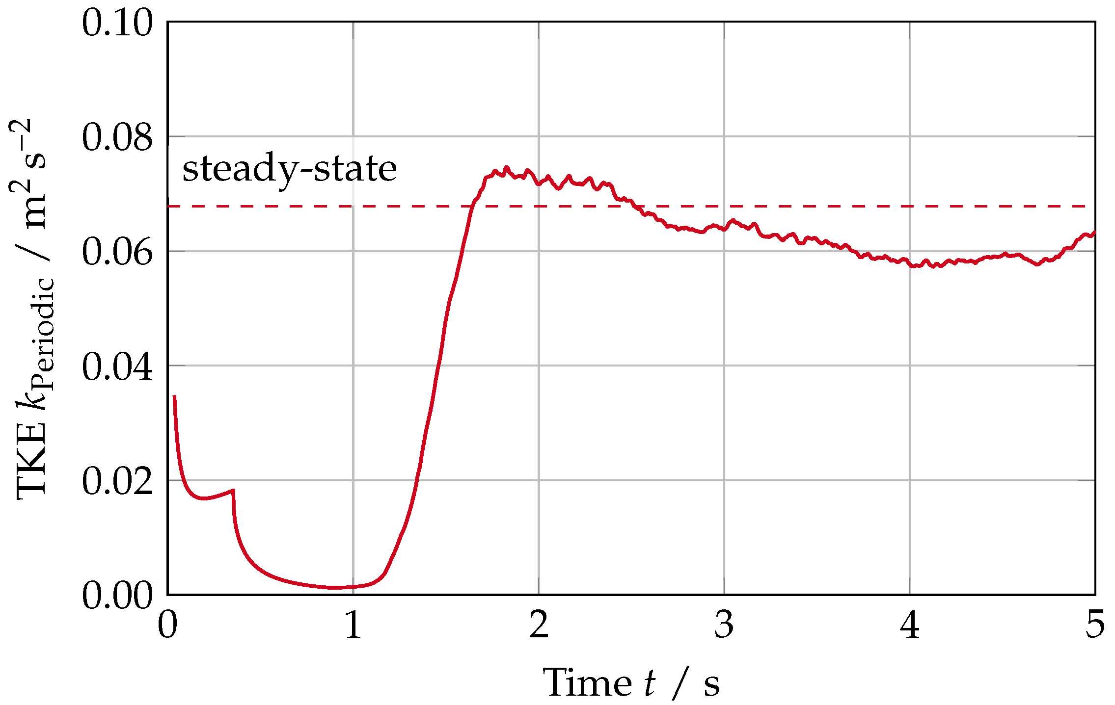
3.1. Computed Initial Solution for the Transient Calculation

Figure 13 shows the flow field used for the initialization of the main transient flow simulation at t = 0 s. In the duct segment, both the periodic and steady-state solutions are interpolated according to Figure 2b. The shown transient solution inside the periodic duct segment is obtained from the periodic duct model, which uses a bigger time step of 1 × 10⁻⁴ s.
As the main purpose of the periodic duct simulation is the generation of a meaningful turbulent inflow boundary condition, the respective development of the TKE on the downstream side of the periodic duct segment is shown in Figure 14. In addition to the transient calculation indicated by the solid line, the TKE on the downstream surface of the periodic duct segment predicted by the steady-state simulation is shown by the dashed line.
The computation of the TKE is based on a sample window of 3838 timesteps or 0.3838 s, which corresponds to roughly three flow cycles through the periodic duct segment. During the first second, no significant turbulent behavior develops, as the flow starts with a homogeneous velocity initial condition. At roughly 1.25 s, the boundary layer develops, and the first stable turbulent scales evolve. After a small overshoot, the TKE then stabilizes at around 5.97 × 10⁻²m2/s2 after about 3.5 s. The computed flow field within the periodic segment after the full initialization period of 5 s is shown in Figure 13. The steady-state solution predicts a TKE level of 6.78 × 10⁻²m2/s2, which is 13.5% higher than the LES solution.
Since the TKE reaches a stable level at the end of the periodic duct simulation, the generated solution is suitable to be used for initialization and the subsequent interpolation with the steady-state solution. The required total time of at least 3.5 s emphasizes the need for the pre-computation of the periodic duct, considering the substantial difference in computational demand for the periodic duct and the full model.

3.2. Validation of the Computed Flow Model Results

To assess if the chosen simulation duration is sufficient for a reliable prediction of the turbulence, the development of the TKE is shown in Figure 15. The ratio of resolved TKE is above 0.85 on both investigated sections (see Figure 15b) across the whole investigated time frame, which indicates sufficient resolution of the turbulent scales. The TKE level on the periodic section for the full transient model is of roughly the same order of magnitude as the periodic duct model (see Figure 14). Since the sampling window for the TKE evaluation during the full transient computation is reduced to 0.05 s, as opposed to 0.3838 s for the “periodic duct” calculation, a deviation from the periodic duct results is to be expected. The TKE level on the diffuser outlet reaches a stationary level from 0.2 s onward. This indicates a proper development of the turbulent flow throughout the whole diffuser, allowing for the start of the acoustic signal sampling.

3.2.1. Aerodynamic Pressure Losses

As the first validation metric, the total-static pressure drop Δ p ts across the diffuser is evaluated for the three-volume flow rates. The corresponding values are summarized in Table 3. To save on computational effort, the pressure drop is evaluated based on steady-state RANS results. A detailed description is given for the operating point of 470 m3/h, where the pressure drop is also evaluated based on the LES results. The measured pressure drop of (33.2 ± 1.2) Pa is close to the value provided by the manufacturer of 32 Pa. The computed pressure drop is evaluated to (33.5 ± 0.3) Pa using the arithmetic mean of the last 0.05 s and reporting the variance in this time frame as uncertainty. The transient LES and steady-state RANS results differ by less than 0.4%, indicating a good estimation of the pressure drop by the RANS calculation. The flow model overpredicts the pressure drop by 3.6–9.0% compared to the experimental results. Since the maximum deviation is below 10%, the aerodynamic losses predicted by the flow model are deemed sufficiently accurate for the investigated volume flow rate.

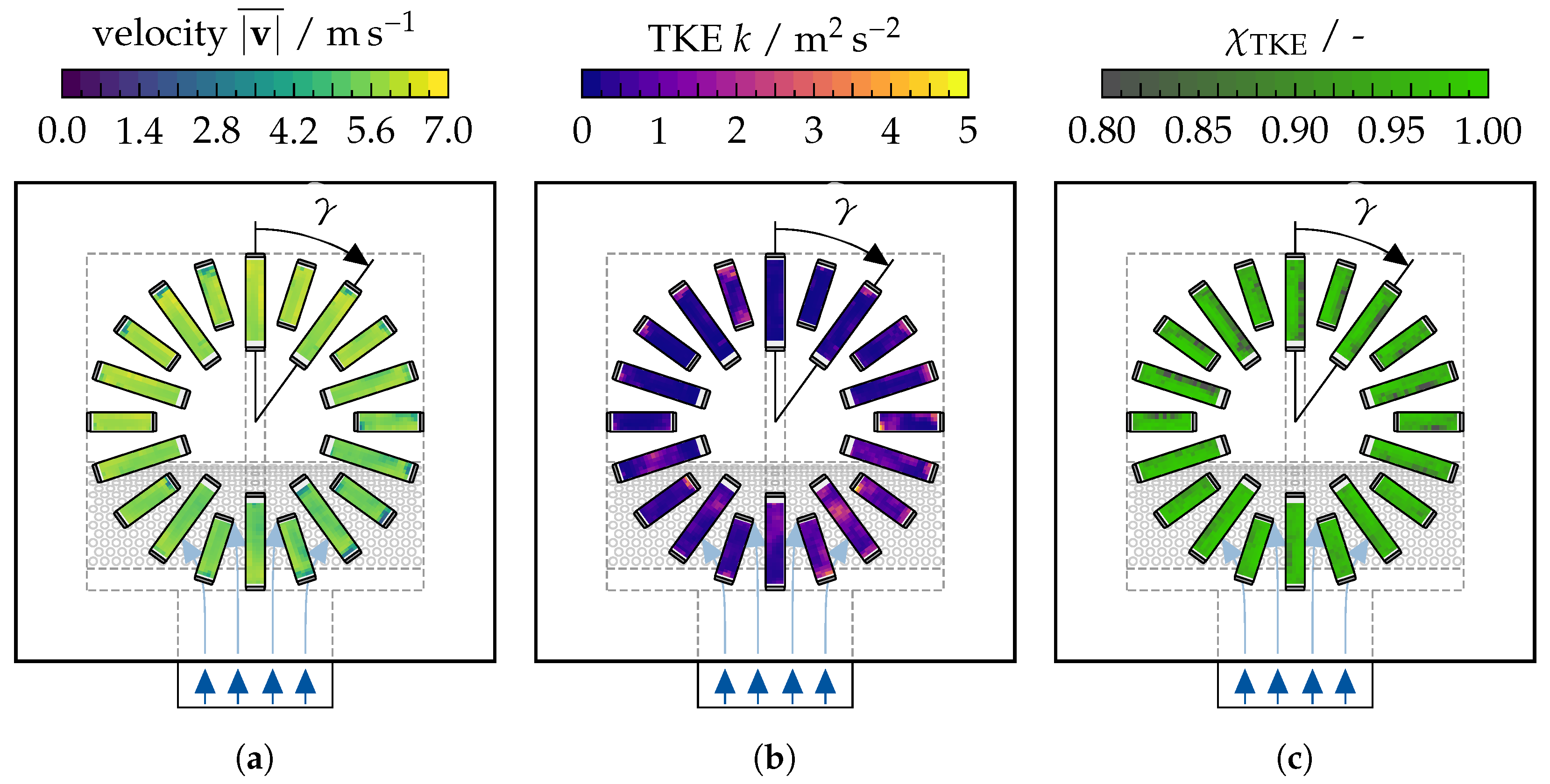
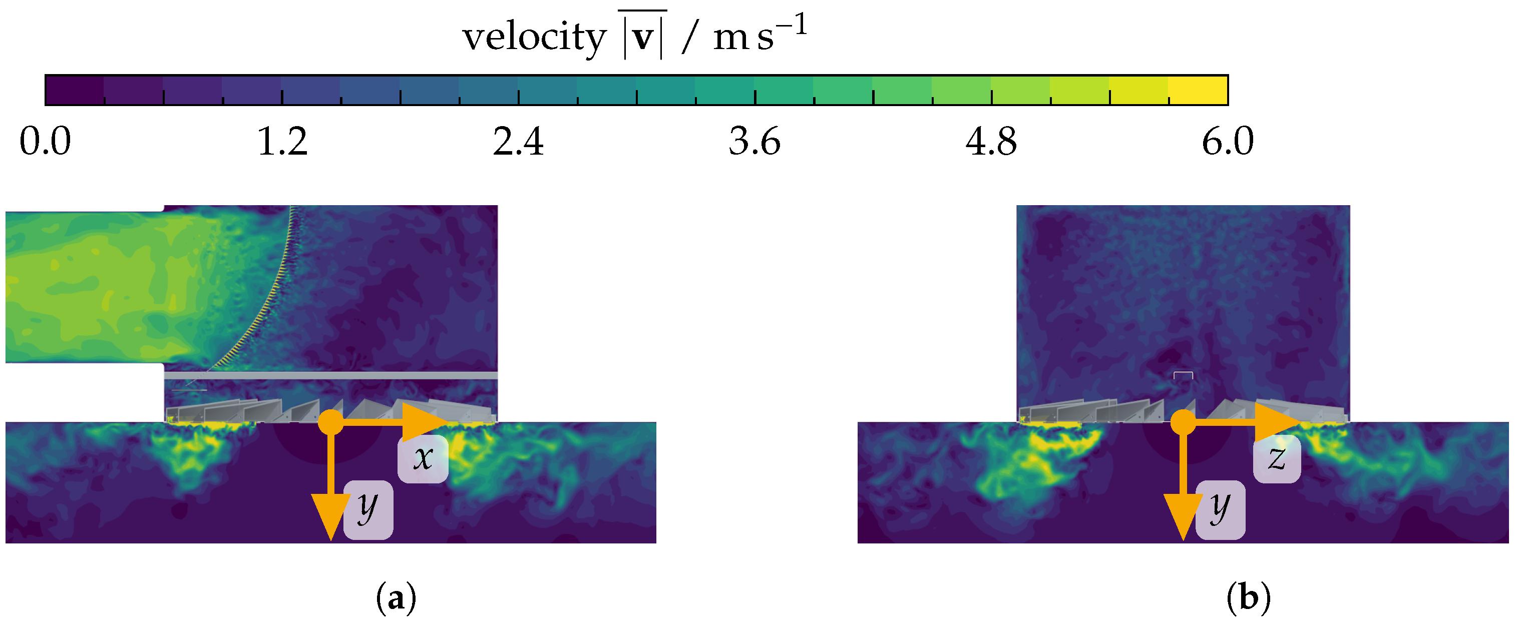
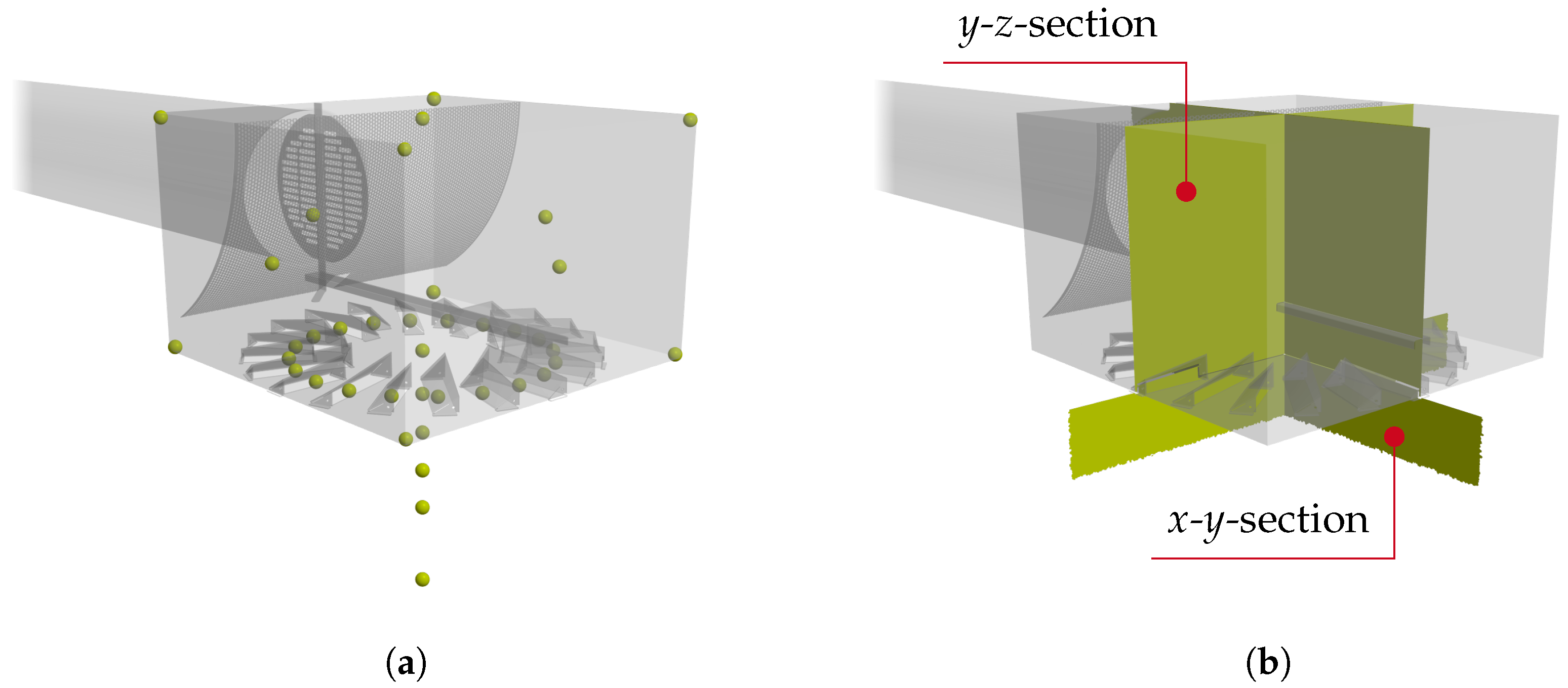
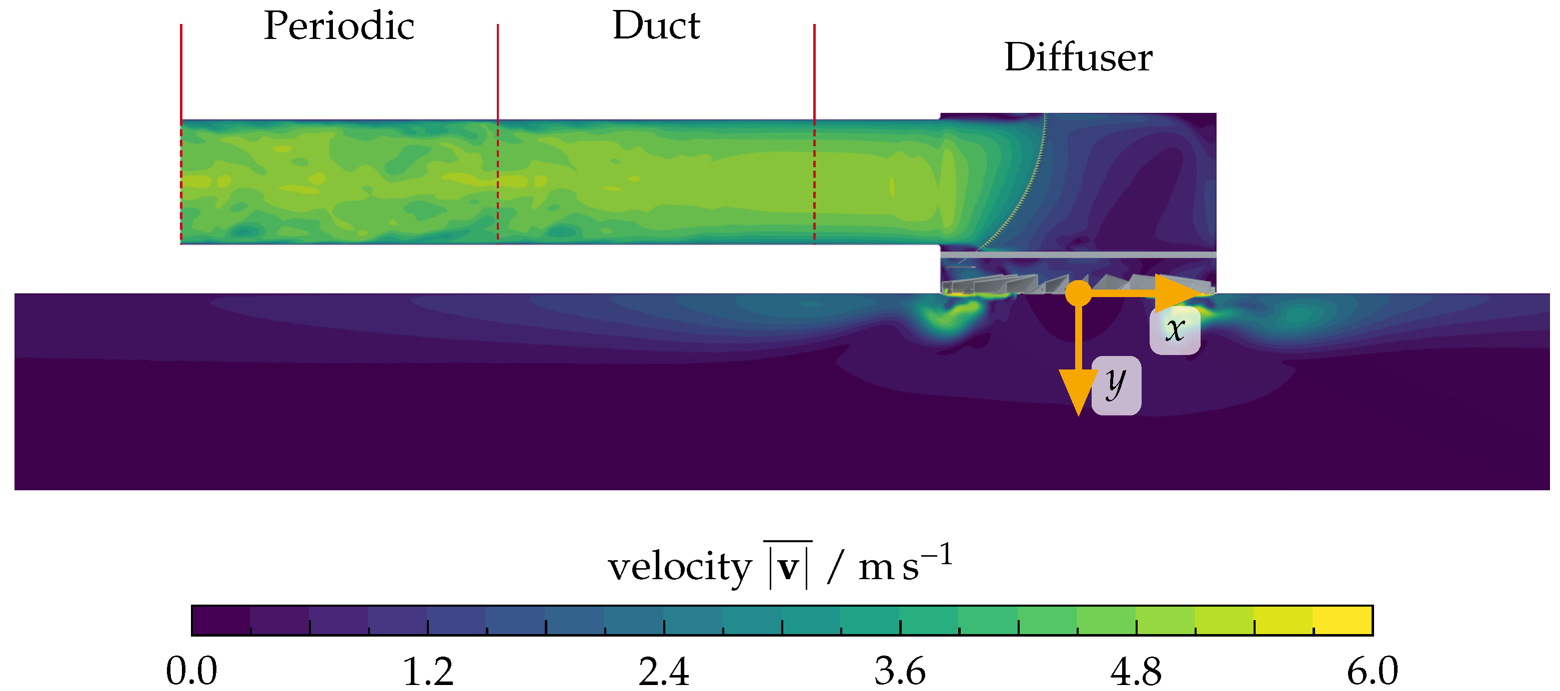
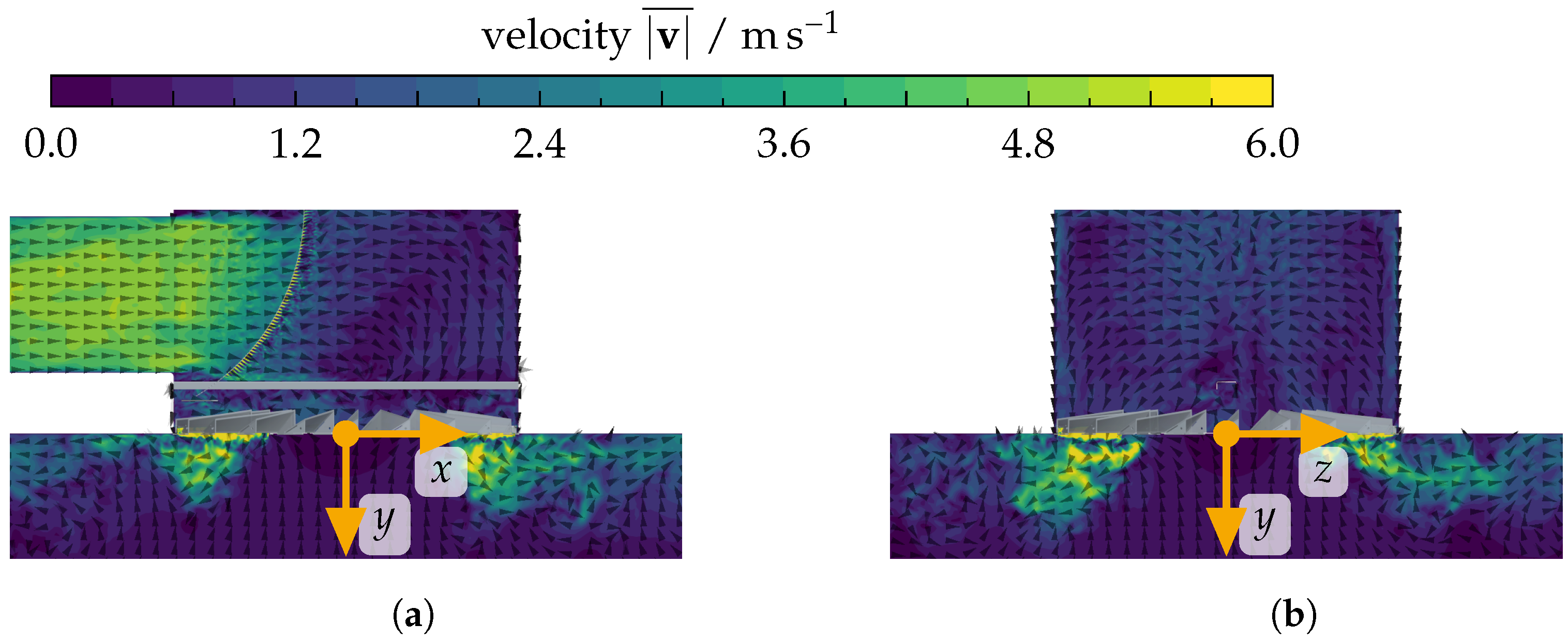
3.2.2. Flow-Field Evaluation

The measured flow field is shown in Figure 16. As can be seen in Figure 16c, the available data rate is low for some measured points. Due to the unpreventable reflections during the LDA measurement that were discussed earlier, a reliable and valid evaluation is not possible here. Only the slots in the range γ = 234–288° (near the 9 o’clock position) achieve a data rate above 700 Hz for at least 80% of the respective points. The other slots are, therefore, neglected for the following validation. In addition to the neglect of the whole slots, the TKE values are computed by further filtering out the individual measurement points that do not satisfy the 700 Hz data rate-criterion.
The remaining four slots are evaluated regarding their average flow velocity, average TKE and volume flow. The same discretization is applied to the LES results, using the time frame from 0.2–0.4 s for calculation of the flow statistics (see Figure A2). As Figure 15 shows, this time frame represents the quasi-stationary flow state. The respective values are summarized in Table 4, with the difference indicating the deviation of the LDA to the LES results.
Both the overall average flow velocity and the volume flow agree well within a tolerance of 10%. Regarding the TKE, only the slot at γ = 252° achieves an error of about 31%. The other slots deviate by a factor of more than two. Since the slot at 252° achieves the highest data rate-validation (only 3.4% of the measurement points are below 700 Hz), the influence of the reflections prevents a successful measurement of the other slots regarding the TKE. Overall, the TKE is underpredicted by about 89.2% in the LES. Due to the uncertainties related to the light reflections caused by the diffuser’s geometry and their impact on the LDA measurement, this big deviation is suspected to emerge from the experimental setup rather than insufficient turbulent development within the simulation.

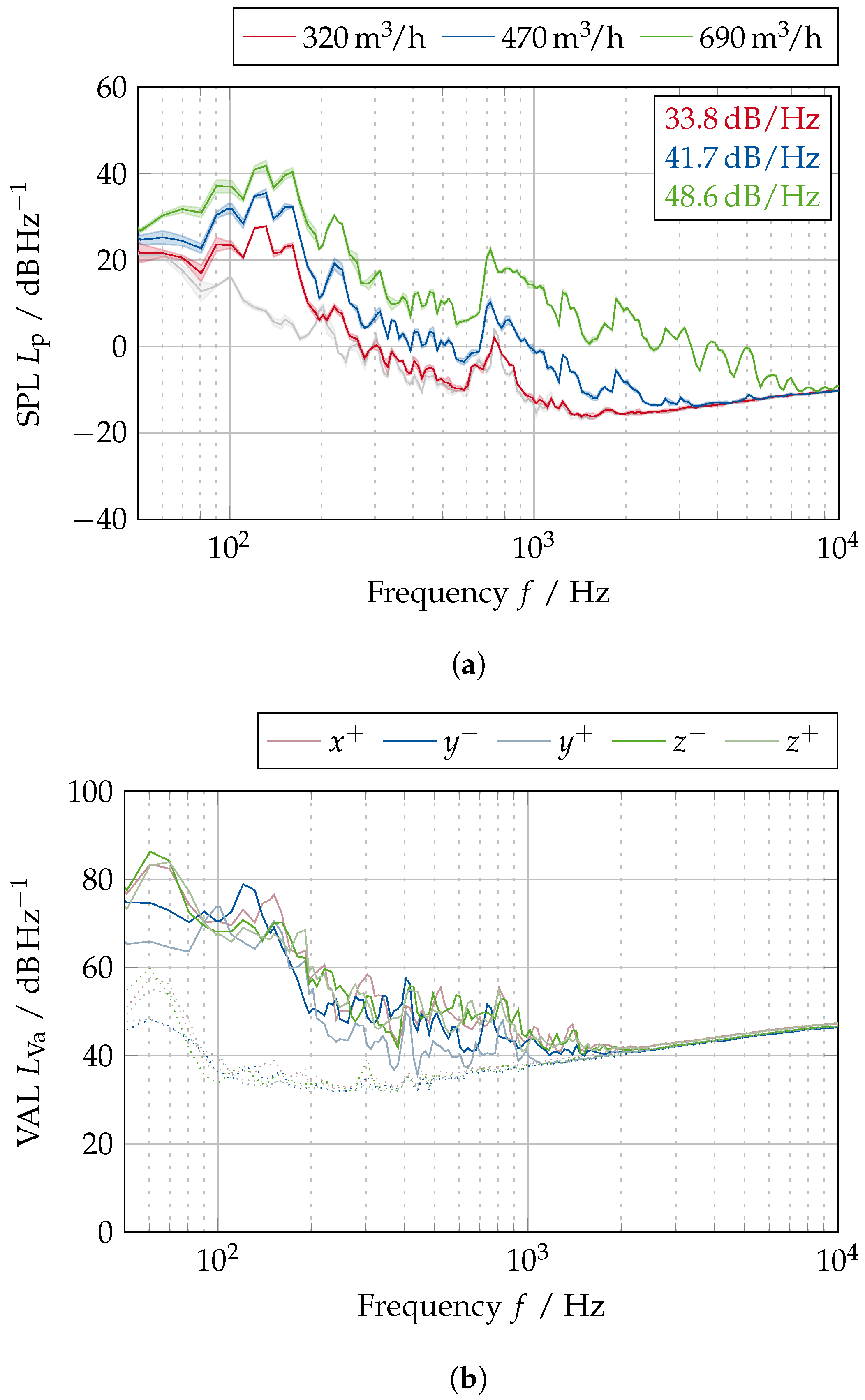
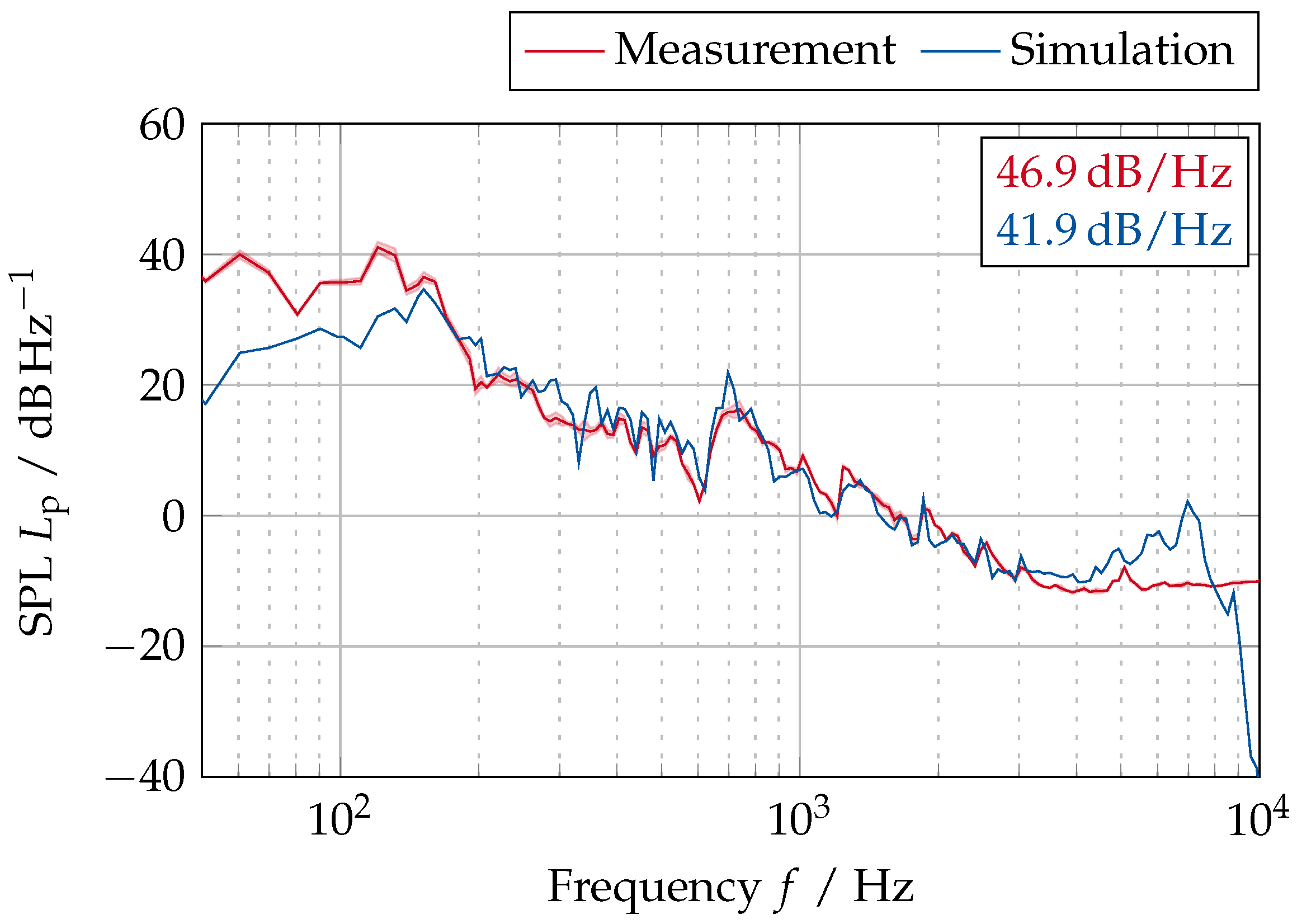
3.2.3. Acoustic Emissions

Figure 17 shows the measured and computed SPL of the acoustic signal as power spectral density in 1 24 -octave bands in a distance of 0.3 m to the diffuser. The OASPLs are summarized inside the plots. The corresponding narrowband spectra are shown in Figure A3. The uncertainty associated with the repeatability of the measurement, indicated by the error band, is below 1.3 dB/Hz in the relevant frequency range.
Regarding the accuracy of the flow model at this position (see Figure 5b) and the characteristics of the measurement chamber, only the frequency range 200–2400 Hz is available for validation. Towards lower frequencies, the computed signal loses accuracy due to the short time frame available for the evaluation of the PSD. Furthermore, the limited space of the measurement chamber and its acoustic properties lead to an attenuation of low-frequency noise. The microphone sensitivity limits the quality of the measured signal towards higher frequencies due to the low signal strength. Since the results are presented as 1 24 -octave bands, this leads to an increase of the SPL towards higher frequencies. Additional results from the measurements, including the evaluation of the acceleration signals, can be found in Figure A6.
Regarding this frequency range (more precisely: 208–2406 Hz) the measured SPL drops by (28.5 ± 0.9) dB/Hz while the computed SPL drops by 26.6 dB/Hz, representing a deviation of 1.8 dB/Hz. Up to 604 Hz the measured and computed SPL features a decline by (17.6 ± 0.9) dB/Hz and 13.2 dB/Hz, respectively.
Near 697 Hz, both the experiment and simulation feature a distinguishable peak. The peak features an increase of (10 ± 90) dB/Hz in the measurement, while the simulation yields a stronger increase of 16.9 dB/Hz.
Within the selected frequency range the computed results are in good agreement with the experimental results. This includes the frequency where the main features occur and their corresponding SPL. The only major exception is the peak near 697, where the simulation overpredicts the peak by 4.1 dB/Hz.

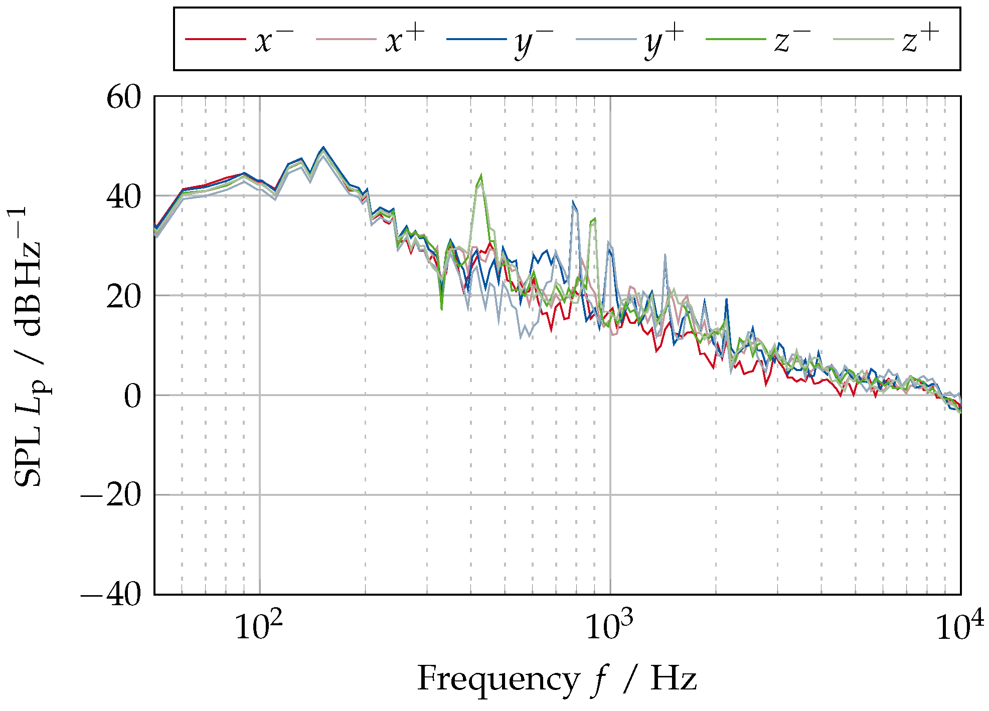
3.3. Simulation Results of the “Base” Model

Figure 18 shows the flow field inside the diffuser at the end of the evaluation time frame at 0.4 s on two cut sections. Both sections are colored according to the flow magnitude. The flow direction is indicated by the cones overlaying the colored sections. Only the flow magnitude is shown in Figure A4. The inbound turbulent flow into the plenum is shown in Figure 18a. The developed pipe flow transitions into a free jet until it reaches the flow homogenizer. Downstream of the flow homogenizer, the flow velocity does not exceed 2 m/s until the flow reaches the guiding elements. The flow homogenizer effectively reduces the overall flow velocity inside the plenum and distributes the airflow evenly on guide elements. When passing the guiding elements, the flow is accelerated to nearly 6 m/s and attaches to the ceiling upon leaving the diffuser. Cutting through the flow field on the y-z-section (see Figure 18b) significant flow structures are visible within the discharge flow only.
Figure 19 shows the PSD of the acoustic pressure sampled at three different receiver locations ( x ; y ; z ) . The first location “0.1 m” at ( 0 ; 0.1 ; 0 ) is already used as a reference location for the acoustic validation presented in Figure 17. Inside the plenum centered above the diffuser plate, the second location “ y ” at ( 0 ; 0.2798 ; 0 ) is in a distance of 5 mm to the respective plenum wall. The third location, “0°” at ( 0.16 ; 0 ; 0 ) , is located inside the outlet section of the guide element opposite the inlet duct. Although the OASPL at the three positions is different, their overall spectral distributions are similar up to a frequency of 300 Hz. Towards higher frequencies, in particular, the signal at location “ y ” features multiple distinguishable peaks. Although a few of those are also visible in the signals of the other two locations, they are not as dominant concerning the respective overall signal. As the power spectral densities of the signals inside the guide element outlet sections and near the plenum walls do not contribute more insight, a detailed description is not given here. However, the corresponding spectra are presented in the appendix (see Appendix C.2).
Figure 20 shows the result of the peak-finding based on the CPSD. As the underlying narrowband signals (see Figure 7) become increasingly noisy at higher frequencies, peak-finding is limited to the range below 4000 Hz. At several frequencies, peaks are present in a large number of CPSD combinations, indicating dominant signal components. The most peaks occur in the 1 24 -octave bands near 428, 587, 698, 1752 and 2699 Hz. Especially the band near 587 Hz features nearly 550 occurrences which is a contribution of 545 741 73.5 % out of all combinations.
Figure 21 and Figure 22 show the evaluation of the SPL on both cut sections for the frequency band near 428 Hz and 587 Hz, respectively. At 428 Hz, the main noise source appears in the upper corners of the z-direction plenum walls, with an imbalance towards the negative z-direction. This indicates that the plenum walls act as a major contributor to the noise emission in this frequency range (see Figure 21b). No large flow structures that potentially act as aeroacoustic sources can be found in either of the identified regions (see Figure A4). This peak is also visible in the measured vibration spectra (see Figure A6b). Furthermore, it is also detected by most of the receivers located in the guide elements (see Figure A7). The large source region in positive z-direction is also slightly visible in the frequency band near 587 Hz (see Figure 22b). Here, a second, stronger source region occurs near the guiding element. As indicated by the respective SPL limits in the corresponding legends, the sources near 428 Hz dominate the sources near 587 Hz by more than 15 dB/Hz, although the peak near 587 Hz occurs in nearly all signals sampled in the guide elements (see Figure A7) as well.
Considering the SPL of the computed signal (see Figure 19), the frequency band near 698 Hz is also worth investigating in more detail. At this frequency, the SPL at the “ y ”-receiver is higher compared to the neighboring frequencies. The corresponding evaluation of the PSD on both cut sections is shown in Figure 23. Here, the region below the mounting beam and the upper corners of the plenum can be identified as the main source regions. Again, the receiver signals in the guide elements (see Figure A7) do feature a range of higher SPL near this frequency band.
All distinguishable peaks occur in the guide elements, although the SPL near the detected frequencies is higher at other positions, such as the plenum walls. The guide elements do contribute to the emission of sound, as an evaluation of the acoustic source terms (see Figure A5) showcases. The generated noise is amplified by the large plenum volume, as no additional sources are visible in the source-term distribution, especially on the y-z-section (see Figure A5b). This amplification is especially strong near the 1st-order eigenmodes (393 and 602 Hz) and the 2nd-order eigenmode in x-/z-direction (786 Hz) of the plenum, which were analytically estimated in a previous study [34].

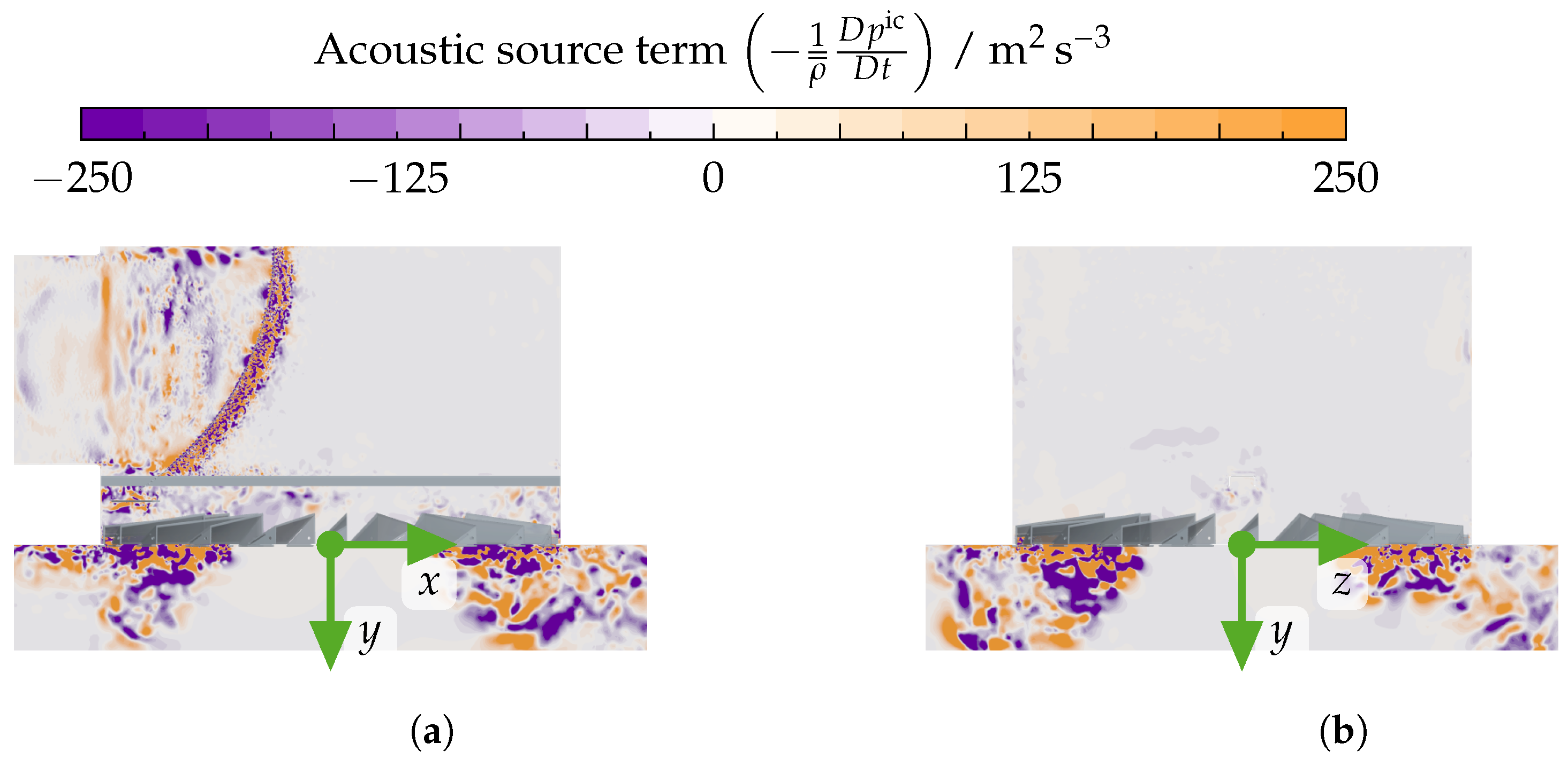
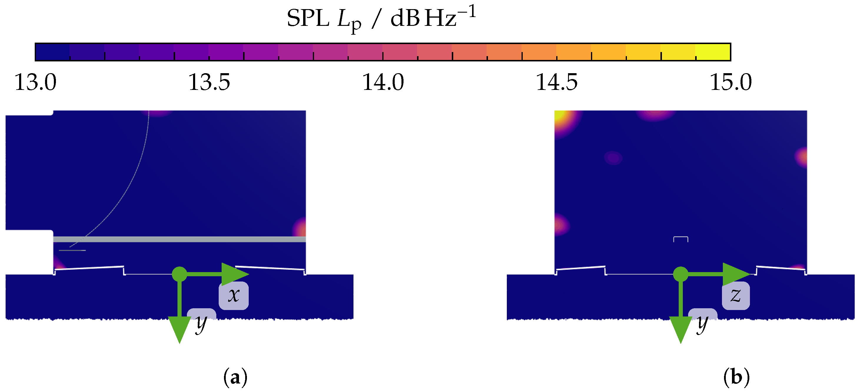
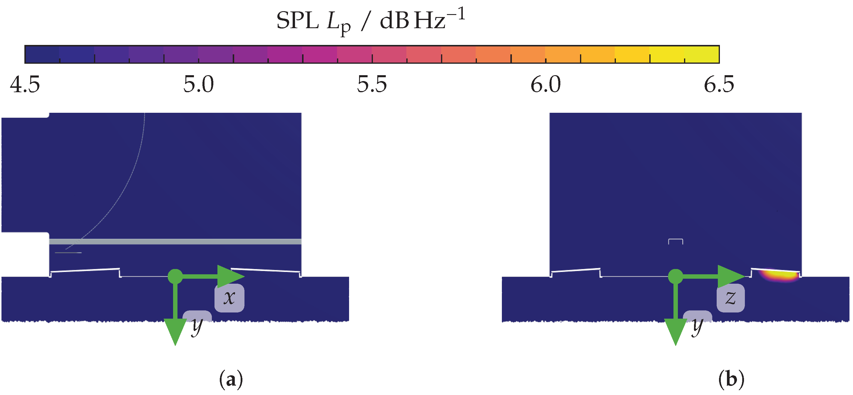
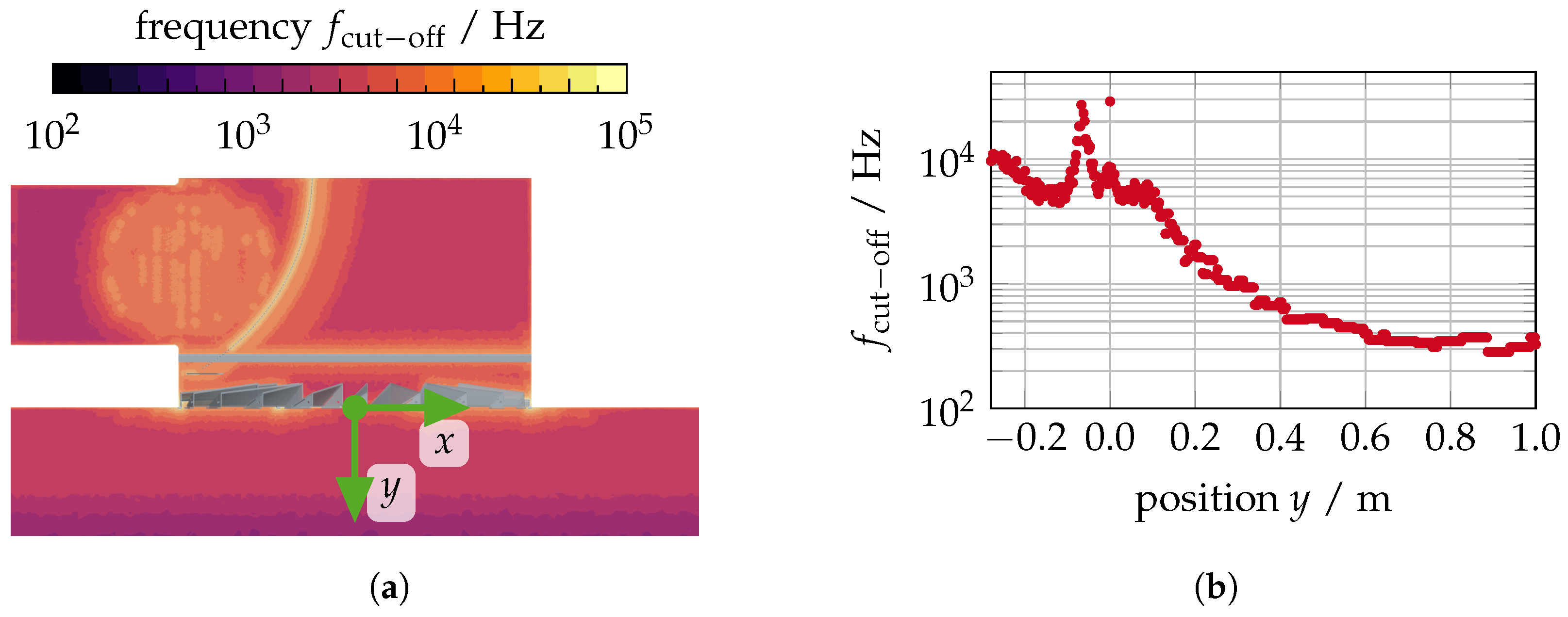
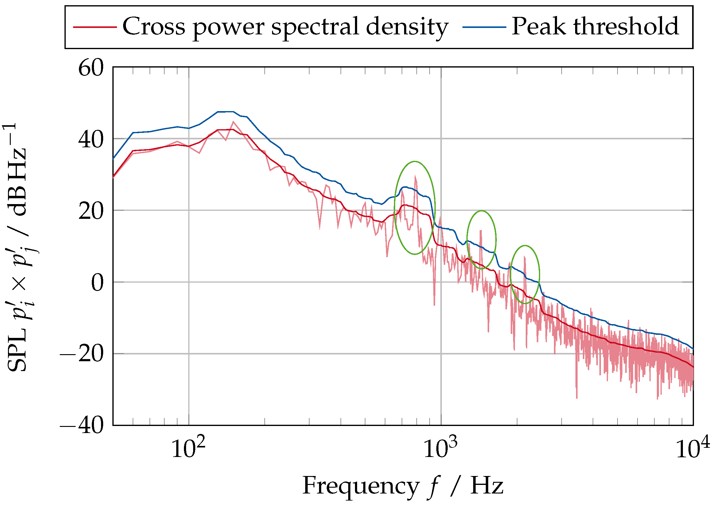
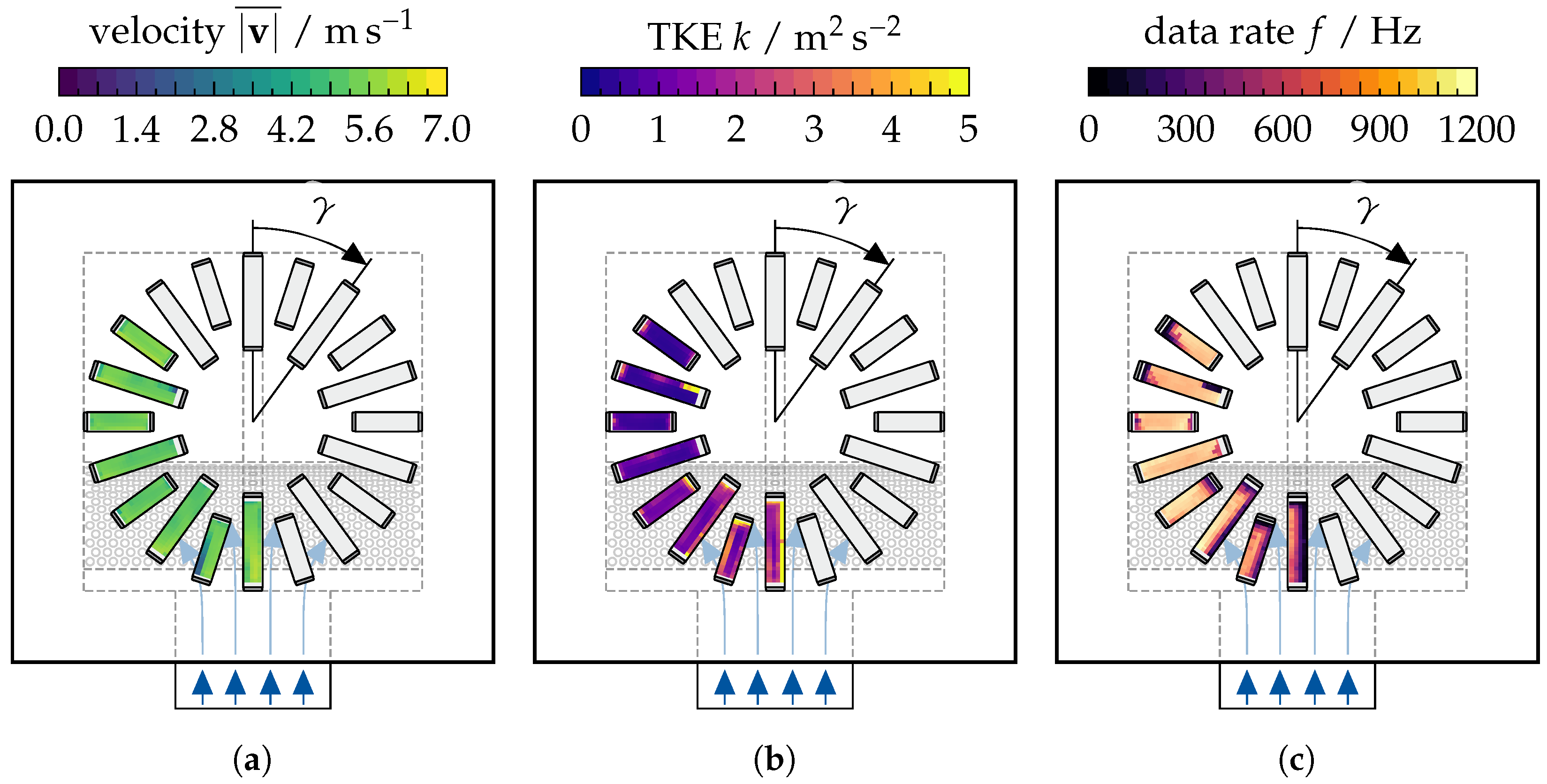
3.4. Identification of Emission Sources

The comparison of the SPL spectra of the acoustic pressure signal 0.1 m below the diffuser of both the “base” and “absorbing” model is shown in Figure 24. The impact of the absorbing plenum walls is strongest in the lower frequency range up to 500 Hz, where the SPL is up to 20 dB Hz−1 lower than the “base” model. Furthermore, the plenum wall receivers feature significantly lower SPL as shown in Figure A8 and Figure A12. The OASPL of the “absorbing” model is reduced by 10 dB/Hz compared to the “base” variant, which is mainly driven by lower SPL at lower frequencies. Up to 600 Hz, the SPL of the “absorbing” model is increasing slightly, as opposed to the decreasing SPL of the “base” model. The peak at 697 Hz does not occur in the case of the “absorbing” model. From 800 Hz onwards, the SPL spectra remain similar to each other.
The additional receiver locations that were already investigated for the “base” model (see Figure 19) are shown in Figure 25 for the “absorbing” model. The y receiver experiences a reduction of the OASPL by nearly 20 dB/Hz compared to the “base” model, yet the y + receiver still features a considerably higher SPL, as shown in Figure A12. Compared to the “base” model, less dominant peaks are visible. Only the range with higher SPL around 800 Hz remains. The SPL spectra of the signals at the 0° and 0.1 m locations are similar to each other, although they switch order regarding their respective SPL from the medium frequency range (below 1000 Hz) towards higher frequencies (above 2000 Hz). The spectra obtained from the receivers inside the guide elements (see Figure A11) are very similar to each other. Especially near 303 Hz they all share a peak with a SPL near 18 dB Hz−1. From 500 Hz, their SPL continuously declines towards higher frequencies.
Figure 26 shows the histogram of peak occurrences for the “absorbing” model in the respective frequency bands. In contrast to the “base” model, practically no peaks occur at 428, 587 and 698 Hz, as the spectra are smoother. The evaluations of the surface SPL at these frequencies are given in the appendix (see Appendix D.2) for the sake of completeness. The most dominant frequency band is shifted to 303 Hz with a contribution of 327 741 44.1 % out of all combinations, which is mainly driven by the receivers inside the guide elements.
The SPL for the frequency band near 303 Hz on both investigated cut sections is shown in Figure 27. Two source regions are in the discharge flow in negative x- and positive z-direction below the diffuser. The same regions feature large turbulent flow structures (see Figure A4b), indicating a coupling between aerodynamic and acoustic phenomena.
Although not identifiable from the CPSD peak-finding, the frequency band near 698 Hz is also evaluated for the “absorbing” model as well, since this was a dominant frequency of the “base” model. The corresponding SPL on both investigated cut sections is shown in Figure 28. In contrast to the “base” model, the sound emission can be attributed to the area near the mounting beam more clearly. This indicates that the source in this frequency band is located there. The absorbing plenum walls reduce the overall SPL near this frequency by 10 dB.
The second most peak occurrences are identified for the frequency band near 2859 Hz, for which the respective surface SPL is shown on both investigated cut sections in Figure 29. In both sections, the guide elements are identified as possible acoustic sources. For the frequency band near 2699 Hz (see Figure A16), the same regions are indicated although less pronounced. The guide element at negative x-direction (location at 180°) features the highest SPL, while the opposite guide element does not feature a visible SPL, given the chosen SPL limits. The “base” model also indicates the guide elements as sources near this frequency band (see Figure A10).
Additional frequency bands of the “reflecting” and “absorbing” variantes are evaluated but only shown in the appendix for the sake of completeness (see Figure A9, Figure A13, Figure A14 and Figure A15).

4. Discussion

The acoustic measurement results are inherent to background noise caused by the limited space of the measurement chamber and the sensitivity of the utilized low-noise microphone. This leads to a limited frequency range between 300–2000 Hz in which the measured results are trustworthy. Many spectral features identified from the (vibro-)acoustic measurements are also found in the simulation results. These include the overall decline of the SPL by 26.6 dB/Hz towards higher frequencies and the various peaks occurring in the spectra. Furthermore, the (vibro-)acoustic results align with their respective counterparts in the simulation, where the plenum wall receivers are considered. Therefore, the numerical model is deemed to be sufficiently accurate to predict the aerodynamic and aeroacoustic behavior of the investigated diffuser. Due to the limited computational resources that were available for this study, a more thorough optimization of the mesh based on transient calculations was not possible. It is expected that a careful definition of the required local refinement regions and the associated analysis of the stepping scheme can reduce the model size further. As the most significant spectral features were found below 5000 Hz, the cut-off frequency could be reduced, thus further reducing the required computational effort.
By computing the model in a “base” and an “absorbing” variant, more detailed insight is obtained into the acoustic source regions that can attenuate certain feedback excitations within the large plenum volume. Since the computational resources are limited, only a short time interval of 0.2 s can be considered for the evaluation of the computed acoustic pressure signals. Although the model is properly initialized before the acoustic sampling begins, the short time frame increases the uncertainty regarding the relative strength of the identified source regions. In particular, the 1st and 2nd-order acoustic eigenmodes of the plenum are found to attenuate the emission near their respective frequency ranges. Since strong sources dominate weaker ones concerning their respective detectable SPL, implementing the plenum walls as absorbing is essential in effectively eliminating the impact of the plenum eigenmodes when identifying the relevant aerodynamically driven source regions. As the flow models do not incorporate structural excitations, only aerodynamic flow structures are left as potential sources for aeroacoustic emission. This renders all identified source regions, which reside in areas of low flow activity, as invalid candidates for potential noise-emitting regions. As such, the regions close to the plenum walls do not originate from aerodynamic processes but are rather linked to acoustic eigenmodes.
The impact of the plenum eigenmodes is primarily assessed by implementing the plenum walls as sound-absorbing and by considering the evaluation of the acoustic source term of the wLPCE approach. As such, especially the strong attenuation near 428 Hz is eliminated in the “absorbing” model and therefore identified as plenum eigenmode. Additionally, no strong acoustic sources are visible from the acoustic source-term evaluation, which further confirms the presence of the eigenmode. In general, the acoustic processes inside the plenum are dominated by the plenum walls and, consequently, the eigenmode attenuation up to a frequency of 500 Hz.
Evaluating the cross-power spectral density for all receivers makes it possible to effectively identify frequency ranges that are dominant across the whole investigated domain. Applying more complex filtering methods or grouping several signals into subgroups according to their locations might lead to an improved extraction of key features of the generated signals. The plenum eigenmodes are detectable from the evaluated histograms of the occurring peaks in the CPSDs.
The imbalances of the SPL on the investigated cut sections are suspected to partly be an artifact of the limited available sampling interval of 0.2 s. The computation of the presented results required about 420.000 core−h on an Intel Xeon Platinum 8160 “SkyLake”-System. An extension of the sampling interval by 0.1 s would increase the computational cost by roughly 80.000 core−h. At the current stage, the additional required computational cost is estimated to outweigh the potential gain in knowledge. However, the presented results are not obtainable by experimental methods. Thus, the application of numerical simulations is crucial in the investigation of the aeroacoustic behavior of air diffusers. It is expected that computational resources, especially in the form of processing units capable of GPGPU, become more widely available in the near future, enabling faster and cheaper computation.
The main limitation of the current state of the presented model is the uncertainty associated with the different locations of both the receiver below the diffuser and the microphone in the experiment. Reducing the distance in the experiment would potentially increase the influence of hydrodynamic pressure fluctuations on the measured acoustic signal. An increase in the distance of the receiver demands a finer mesh and, therefore, would increase the already substantial computational cost. The presented approach is therefore a tradeoff between cost and ability of the model to capture the main characteristics of the investigated diffuser.

5. Conclusions

In its “base” variant, the flow model predicts the aeroacoustic spectrum with key features like dominant frequency ranges in good agreement to (vibro-)acoustic measurements. The plenum is identified as a main source of aeroacoustic emissions, although the plenum is implemented with perfectly stiff walls without the required degree of freedom of vibrations that would satisfy this conclusion. By applying a sound-absorbing boundary condition to the plenum walls, the discharge flow (near 303 Hz), the mounting beam (near 698 Hz), and the guide elements (near 2859 Hz) are identified as major, aerodynamically driven sound emission sources. All sources feature a broadband characteristic that excites certain eigenmodes of the plenum, leading to an attenuation of the signal near 428 Hz. Combining an evaluation of the CPSD to identify dominant frequency ranges with a subsequent investigation of the SPL at certain frequency bands on cut sections is a suitable tool to identify aeroacoustic sources emerging from geometric features. Based on the identified geometric features that contribute the most to the noise emission, geometric modifications can be derived to alter the emission characteristic of the diffuser.
The size of the presented model requires a substantial amount of memory during calculation. Suitable processing units capable of GPGPU that can handle this model size with a manageable number of units have been available for a few years. Therefore, the presented methodology is expected to become more viable in the next few years, especially if future studies focus on optimizing the mesh size distribution further.

Author Contributions

Conceptualization, P.O.; Data curation, P.O.; Formal analysis, P.O.; Funding acquisition, D.M.; Investigation, P.O.; Methodology, P.O.; Project administration, M.K. and D.M.; Resources, P.O.; Software, P.O.; Supervision, M.K. and D.M.; Validation, P.O. and M.K.; Visualization, P.O.; Writing—original draft, P.O.; Writing—review and editing, P.O., M.K., and D.M. All authors have read and agreed to the published version of the manuscript.

Funding

Grateful acknowledgment is made for financial support by the German Federal Ministry for Economic Affairs and Climate Action (BMWK), the DLR-Projektträger, and the “Forschungsvereinigung für Luft und Trocknungstechnik (FLT) e. V.”, promotional reference 21611 N.

Institutional Review Board Statement

Not applicable.

Informed Consent Statement

Not applicable.

Data Availability Statement

The data presented in this study are available on request from the corresponding author due to the large size of the simulation and result files.

Acknowledgments

The authors gratefully acknowledge the computing time provided to them at the NHR Center NHR4CES at RWTH Aachen University (project number p0020083). This is funded by the Federal Ministry of Education and Research, and the state governments participating on the basis of the resolutions of the GWK for national high-performance computing at universities (www.nhr-verein.de/unsere-partner).

Conflicts of Interest

The authors declare no conflicts of interest.

Abbreviations

The following abbreviations are used in this manuscript:
AHUAir handling unit
APEAcoustic Perturbed Equation
BPFBlade passing frequency
CAAComputational Aeroacoustics
CFDComputational Fluid Dynamics
CPSDCross-Power spectral density
FW-HFfowcs–Williams Hawkings
GUMGuide to the expression of uncertainty in measurement
LDALaser-Doppler-Anemometry
LESLarge-Eddy Simulation
OASPLOverall sound-pressure level
PPWpoints per wavelength
PSDPower spectral density
RANSReynolds-Averaged Navier–Stokes
SPLSound-pressure level
TKETurbulent Kinetic Energy
WALEWall-Adapting Local-Eddy Viscosity
wLPCEwave Linearized Perturbed Compressible Equation

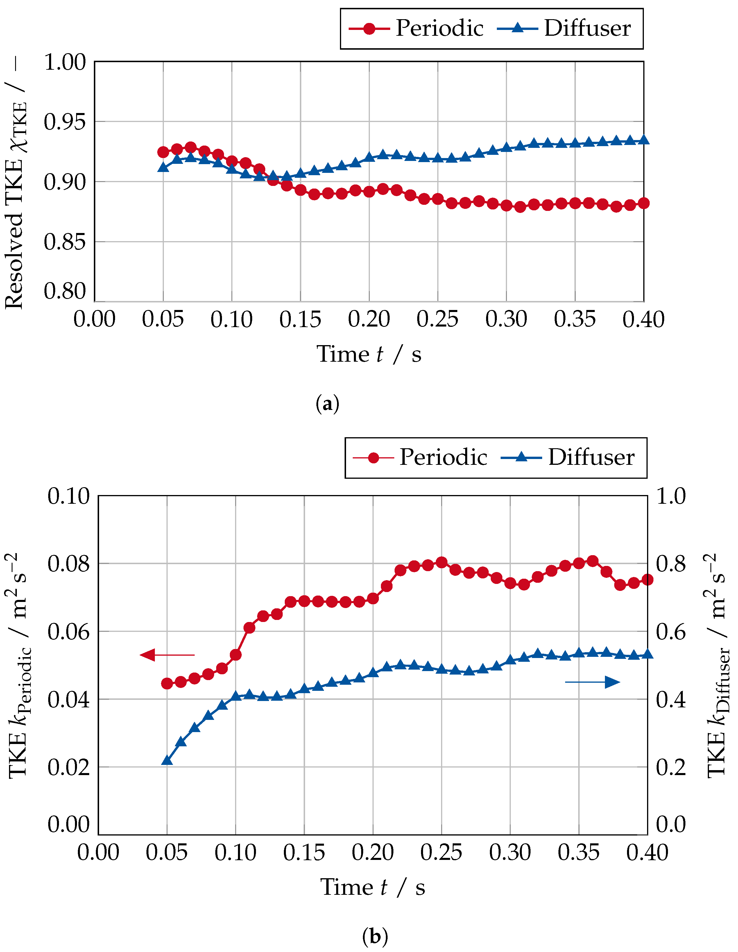
Appendix A. Evaluation of the Turbulent Kinetic Energy

The velocity field is sampled on two evaluation sections (“Periodic” and “Diffuser”), shown in Figure A1. By design, the LES only captures flow scales that are resolved by the computational mesh. Turbulent structures smaller than the mesh resolution are modeled by the subgrid-scale model. The overall TKE k is the combination of resolved turbulence k Var based on the velocity variance v 2 ¯ and the modeled portion of the subgrid-scale model k SGS according to Equation (A1). Here, v is not to be mistaken with the acoustic velocity.
k = k Var + k SGS ¯ = 1 2 v x 2 ¯ + v y 2 ¯ + v z 2 ¯ + k SGS ¯
The average flow velocity v ¯ Equation (A2) and the velocity variance v 2 ¯ Equation (A3) are computed using the same sampling window and resolution. The subgrid-scale TKE is averaged in the same fashion as the average flow velocity.
v i ¯ = 1 N j = 1 N v i
v i 2 ¯ = 1 N j = 1 N v i v i ¯ 2
The ratio of resolved turbulence r TKE indicates how much of the TKE is resolved directly by the LES related to the total TKE as shown in Equation (A4). The ratio should generally be above 0.8 to indicate sufficient resolution of the flow model [62].
χ TKE = k Var k Var + k SGS ¯ = k Var k CFD
Figure A1. Overview of the sections used for evaluation of the flow-field statistics. (a) Downstream side of the periodic duct segment. (b) Diffuser outlet into the room.
Acoustics 07 00009 g0a1

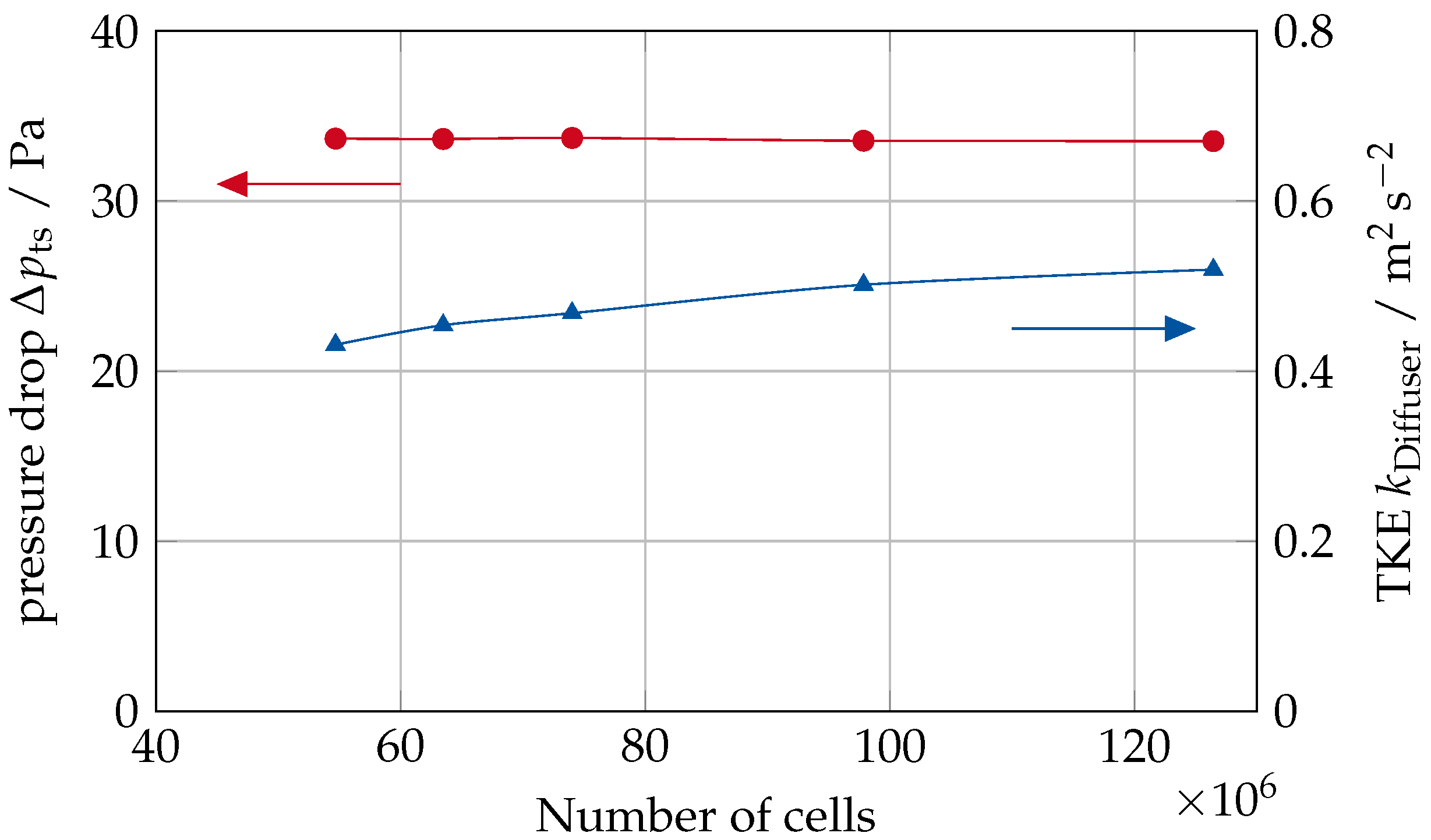
Appendix B. Results of the Mesh Independence Study

The computational mesh consists of multiple surface and volumetric refinement zones. In order to rate the mesh independence, the refinement of the flow homogenizer and the guide elements was incrementally changed to generate several meshes. The smallest mesh further featured a coarser resolution of the plenum and outflow region. Figure 4 shows the dependency of the pressure loss and the turbulent kinetic energy on the outlet section of the diffuser. While no clear dependency on the mesh is observable for the pressure loss, the turbulent kinetic energy requires a fine resolution in the vicinity of the flow homogenizer and the guide elements. As the mesh independence study was performed on the basis of steady-state RANS simulations, it is to be expected that the transient LES calculations require at least the finest resolution that was investigated to achieve good results.

Appendix C. Additional Evaluation of the “Base” Model

Figure A2. Overview of the flow-field results based on the LES results. (a) Velocity; (b) Turbulence; (c) resolved Turbulence.
Acoustics 07 00009 g0a2
Figure A3. Comparison of the narrowband power spectral density of the measured and computed acoustic pressure for 470 m3/h. Towards higher frequencies the sensitivity limit of the microphone leads to an increase of sound-pressure level for the measurement.
Acoustics 07 00009 g0a3
Figure A4. Velocity field for the “base” model on the x-y- and y-z-section at t = 0.4 s. The flow enters the plenum from the negative x-direction and exits through the diffuser plate in the positive y-direction. (a) x-y-section at z = 0 m. (b) y-z-section at x = 0 m.
Acoustics 07 00009 g0a4
Figure A5. Instantaneous distribution of the acoustic source-term Equation (10) on both cut sections for the “base” model at t = 0.4 s. (a) x-y-section at z = 0 m. (b) y-z-section at x = 0 m.
Acoustics 07 00009 g0a5

Appendix C.1. Measurement Results

Figure A6. Measured sound-pressure level and vibration acceleration level in 1 24 -octave bands. (a) Sound-pressure level of the measured acoustic pressure in a distance of 1.5m. The reference calm measurement is colored in gray. (b) Vibration acceleration level of the measured accelerations on the plenum walls for 470 m3/h. The reference calm measurement is indicated by the dotted lines.
Acoustics 07 00009 g0a6

Appendix C.2. Sound-Pressure Level at Additional Receiver Locations for the “Base” Model

Figure A7. Comparison of the sound-pressure level in 1 24 -octave bands at all guide element receiver locations. The data are colored in ascending order from red (at 0°) to gray (at 342°).
Acoustics 07 00009 g0a7
Figure A8. Comparison of the sound-pressure level in 1 24 -octave bands at all plenum wall receiver locations.
Acoustics 07 00009 g0a8

Appendix C.3. Evaluation of the Surface Sound-Pressure Level at Additional Frequency Bands for the “Base” Model

Figure A9. Sound-pressure level on both cut sections for the 1 24 -octave band at 1753 Hz. (a) x-y-section at z = 0 m. (b) y-z-section at x = 0 m.
Acoustics 07 00009 g0a9
Figure A10. Sound-pressure level on both cut sections for the 1 24 -octave band at 2699 Hz. (a) x-y-section at z = 0 m. (b) y-z-section at x = 0 m.
Acoustics 07 00009 g0a10

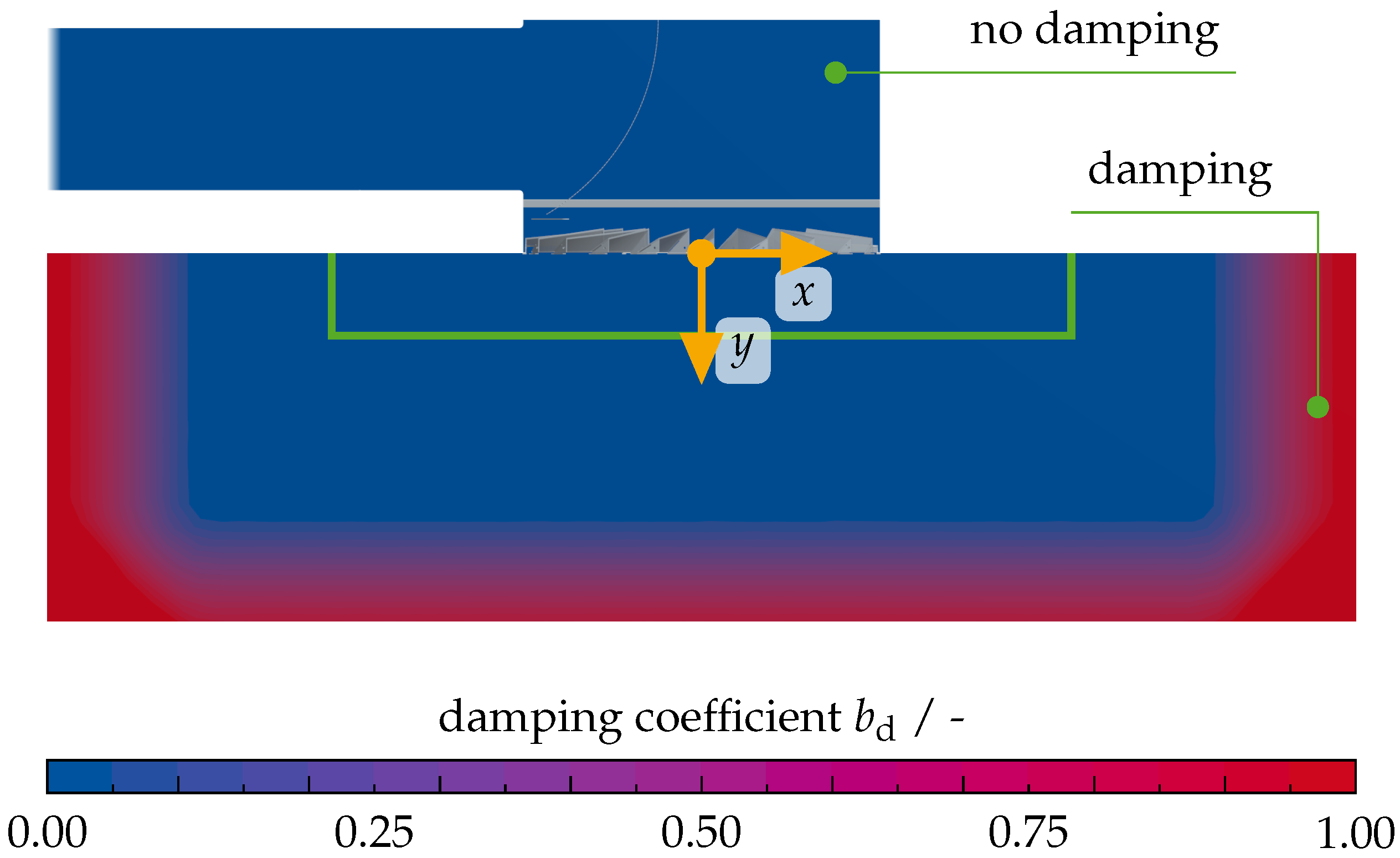
Appendix D. Additional Evaluation of the “Absorbing” Model

Appendix D.1. Sound-Pressure Level at Additional Receiver Locations for the “Absorbing” Model

Figure A11. Comparison of the sound-pressure level in 1 24 -octave bands at all guide element receiver locations. The data are colored in ascending order from red (at 0°) to gray (at 342°).
Acoustics 07 00009 g0a11
Figure A12. Comparison of the sound-pressure level in 1 24 -octave bands at all plenum wall receiver locations.
Acoustics 07 00009 g0a12

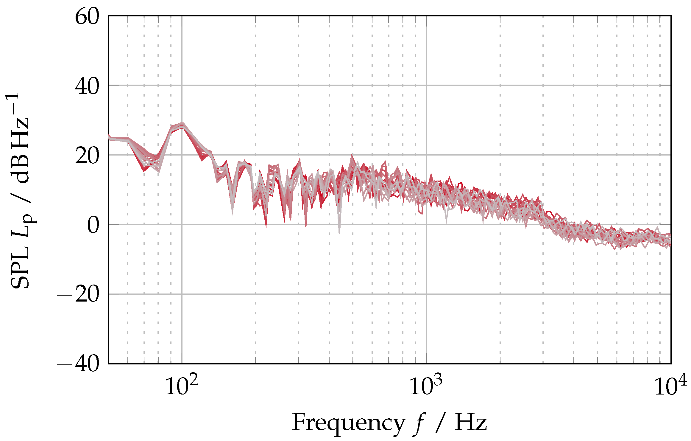
Appendix D.2. Evaluation of the Surface Power Spectral Density at Additional Frequency Bands for the “Absorbing” Model

Figure A13. Sound-pressure level on both cut sections for the 1 24 -octave band at 428 Hz for the “absorbing” model. (a) x-y-section at z = 0 m. (b) y-z-section at x = 0 m.
Acoustics 07 00009 g0a13
Figure A14. Sound-pressure level on both cut sections for the 1 24 -octave band at 587 Hz for the “absorbing” model. (a) x-y-section at z = 0 m. (b) y-z-section at x = 0 m.
Acoustics 07 00009 g0a14
Figure A15. Sound-pressure level on both cut sections for the 1 24 -octave band at 1753 Hz. (a) x-y-section at z = 0 m. (b) y-z-section at x = 0 m.
Acoustics 07 00009 g0a15
Figure A16. Sound-pressure level on both cut sections for the 1 24 -octave band at 2699 Hz. (a) x-y-section at z = 0 m. (b) y-z-section at x = 0 m.
Acoustics 07 00009 g0a16

References

  1. Bundesanstalt für Arbeitsschutz und Arbeitsmedizin. Technische Regeln Für Arbeitsstätten. Lärm. 2021.
  2. Winkelmann, S.; Stürenburg, L.; Schiller, I.; Fels, J.; Schlittmeier, S. Subjektiver Akustischer Komfort von Luftdurchlässen Für Gebäudebelüftungen. In Proceedings of the Fortschritte Der Akustik—DAGA 2023, Hamburg, Germany, 6–9 May 2023. [Google Scholar]
  3. Stürenburg, L.; Ostmann, P.; Aspöck, L.; Fels, J.; Müller, D. Acoustic measurements and psychoacoustic analyses of ventilation diffusers. In Proceedings of the INTER-NOISE and NOISE-CON Congress and Conference Proceedings, Glasgow, UK, 21–24 August 2022. [Google Scholar] [CrossRef]
  4. Stürenburg, L.; Ostmann, P.; Aspock, L.; Müller, D.; Fels, J. Herausforderungen bei Messungen von Lüftungsgeräuschen in einem reflexionsfreien Halbraum. In Proceedings of the Fortschritte der Akustik—DAGA 2024, Hannover, Germany, 18–21 May 2024. [Google Scholar]
  5. Ffowcs Williams, J.E.; Hawkings, D.L. Sound Generation by Turbulence and Surfaces in Arbitrary Motion. Math. Phys. Sci. 1969, 264, 321–342. [Google Scholar]
  6. Ewert, R.; Schröder, W. Acoustic Perturbation Equations Based on Flow Decomposition via Source Filtering. J. Comput. Phys. 2003, 188, 365–398. [Google Scholar] [CrossRef]
  7. Seo, J.H.; Moon, Y.J. Perturbed Compressible Equations for Aeroacoustic Noise Prediction at Low Mach Numbers. AIAA J. 2005, 43, 1716–1724. [Google Scholar] [CrossRef]
  8. Seo, J.H.; Moon, Y.J. Linearized Perturbed Compressible Equations for Low Mach Number Aeroacoustics. J. Comput. Phys. 2006, 218, 702–719. [Google Scholar] [CrossRef]
  9. Hüppe, A. Spectral Finite Elements for Acoustic Field Computation; Measurement-, Actuator-, and Simulation-Technology, Shaker: Aachen, Germany, 2013. [Google Scholar] [CrossRef]
  10. Piepiorka, J.; von Estorff, O. Numerical Investigation of Hydrodynamic/Acoustic Splitting Methods in Finite Volumes Including Rotating Domains. In Proceedings of the 23rd International Congress on Acoustics, Aachen, Germany, 9–13 September 2019; pp. 1827–1834. [Google Scholar]
  11. Ocker, C.; Geyer, T.F.; Czwielong, F.; Krömer, F.; Becker, S.; Merkel, M.; Pannert, W. Experimental Investigation of the Impact of 3D-Metal-Printed Perforated Leading Edges on Airfoil and Axial Fan Noise. In Proceedings of the AIAA Aviation 2020 Forum, Virtual Event, 15–19 June 2020. [Google Scholar] [CrossRef]
  12. Ocker, C.; Czwielong, F.; Chaitanya, P.; Pannert, W.; Becker, S. Aerodynamic and Aeroacoustic Properties of Axial Fan Blades with Slitted Leading Edges. Acta Acust. 2022, 6, 48. [Google Scholar] [CrossRef]
  13. Czwielong, F.; Berchtenbreiter, B.; Ocker, C.; Geyer, T.; Stockmeier, G.; Merkel, M.; Becker, S. On the Application and Limitations of Sound-Absorbing Materials for Axial Fan Blades. In Proceedings of the Fan 2022–International Conference on Fan Noise, Aerodynamics, Applications and Systems, Senlis, France, 27–29 June 2022. [Google Scholar] [CrossRef]
  14. Clark, I.A.; Alexander, W.N.; Devenport, W.; Glegg, S.; Jaworski, J.W.; Daly, C.; Peake, N. Bioinspired Trailing-Edge Noise Control. AIAA J. 2017, 55, 740–754. [Google Scholar] [CrossRef]
  15. Lendvai, B.; Benedek, T. Experimental and Numerical Investigation of the Blade Tip-Related Aeroacoustic Sound Source Mechanisms of a Ducted Low-Speed Axial Flow Fan. Appl. Acoust. 2024, 215, 109705. [Google Scholar] [CrossRef]
  16. Sun, Z.; Tian, J.; Zheng, Y.; Zhu, X.; Du, Z.; Ouyang, H. Design of Sinusoidal-Shaped Inlet Duct for Acoustic Mode Modulation Noise Reduction of Cooling Fan. Appl. Acoust. 2024, 216, 109741. [Google Scholar] [CrossRef]
  17. Lörcher, F.; Hub, S. Effizientes Und Schallarmes Axialventilatorsystem Mit Neuartigem Zonal Optimiertem Nachleitrad. In Proceedings of the Fortschritte Der Akustik—DAGA 2023, Hamburg, Germany, 6–9 May 2023; pp. 1564–1567. [Google Scholar]
  18. Schäfer, R.; Böhle, M. Validation of the Lattice Boltzmann Method for Simulation of Aerodynamics and Aeroacoustics in a Centrifugal Fan. Acoustics 2020, 2, 735–752. [Google Scholar] [CrossRef]
  19. Tautz, M. Aeroacoustic Noise Prediction of Automotive HVAC Systems. Ph.D. Thesis, FAU University Press, Erlangen, Germany, 2019. [Google Scholar] [CrossRef]
  20. Yadegari, M.; Ommi, F.; Karimian Aliabadi, S.; Saboohi, Z. Reducing the Aerodynamic Noise of the Axial Flow Fan with Perforated Surface. Appl. Acoust. 2024, 215, 109720. [Google Scholar] [CrossRef]
  21. Zurbano-Fernández, I.; Guedel, A.; Robitu, M.; Roger, M. Noise Reduction of a Centrifugal Plenum Fan with Leading Edge or Trailing Edge Serrations. In Proceedings of the Fan 2022—International Conference on Fan Noise, Aerodynamics, Applications and Systems, Senlis, France, 27–29 June 2022. [Google Scholar] [CrossRef]
  22. Perot, F.; Kim, M.S.; Freed, D.; Lee, D.; Ih, K.D.; Ih, K.D.; Kim, M.S. Direct Aeroacoustics Prediction of Ducts and Vents Noise. In Proceedings of the 16th AIAA/CEAS Aeroacoustics Conference, Reston, Virigina, Stockholm, Sweden, 7–9 June 2010. [Google Scholar] [CrossRef]
  23. Curle, N. The Influence of Solid Boundaries upon Aerodynamic Sound. Proc. R. Soc. Lond. Ser. Math. Phys. Sci. 1955, 231, 505–514. [Google Scholar] [CrossRef]
  24. Proudman, I. The Generation of Noise by Isotropic Turbulence. Proc. R. Soc. Lond. Ser. Math. Phys. Sci. 1952, 214, 119–132. [Google Scholar] [CrossRef]
  25. Khondge, A.D.; Sovani, S.D.; Kim, S.E.; Guzy, S.C.; Farag, A.A. On Predicting Aeroacoustic Performance of Ducts with Broadband Noise Source Models. In SAE Technical Paper Series; SAE International: Warrendale, PA, USA, 2005. [Google Scholar] [CrossRef]
  26. Mohamud, O.M.; Johnson, P. Broadband Noise Source Models as Aeroacoustic Tools in Designing Low NVH HVAC Ducts. In SAE Technical Paper Series; SAE International: Warrendale, PA, USA, 2006. [Google Scholar] [CrossRef]
  27. Ravichandran, A.; Logdesser, A.; Peller, N.; Manhart, M. Experimentelle Und Numerische Untersuchung Des Effekts Der Zuströmbedingungen Auf Die Schallabstrahlung Eines Generischen Ausströmers. In Proceedings of the Fortschritte Der Akustik—DAGA 2022, Stuttgart und Online, 21–24 May 2022; pp. 1250–1253. [Google Scholar]
  28. Ravichandran, A.; Manhart, M.; Schwertfirm, F.; Peller, N. Wake Flow-Acoustic Resonance in a Generic Air Outlet. In Proceedings of the TSFP12, Osaka, Japan, 19–22 July 2022. [Google Scholar]
  29. Ewert, R.; Kreuzinger, J. Hydrodynamic/Acoustic Splitting Approach with Flow-Acoustic Feedback for Universal Subsonic Noise Computation. J. Comput. Phys. 2021, 444, 110548. [Google Scholar] [CrossRef]
  30. Fenini, L. Numerical Modelling Of Flow-Induced Noise Emitted by Control Devices. Ph.D. Thesis, Politecnico Di Milano, Mailand, Italy, 2019. [Google Scholar]
  31. Bechara, W.; Bailly, C.; Lafon, P.; Candel, S.M. Stochastic Approach to Noise Modeling for Free Turbulent Flows. AIAA J. 1994, 32, 455–463. [Google Scholar] [CrossRef]
  32. Saarinen, P.; Koskela, H. Flow Noise from an Exhaust Valve - Prediction by Simulations as Compared with Measurements. In Proceedings of the 12th International Conference on Air Distribution in Rooms, Austin, TX, USA, 5–10 June 2011. [Google Scholar]
  33. Saarinen, P.; Mustakallio, P. Simulation of Flow Noise Generation in a Circular Ceiling Diffuser: A Comparison Between a Silent and a Noisy Design by Using CFD and Lighthill’s Acoustic Analogy. In Proceedings of the ISHVAC 2011, Shanghai, China, 6–9 November 2011. [Google Scholar]
  34. Ostmann, P.; Krüger, L.; Kremer, M.; Müller, D. Contribution of Geometric Features on the Aeroacoustic Behaviour of a Slot Diffuser. In Proceedings of the 36th International Conference on Efficiency, Cost, Optimization, Simulation and Environmental Impact of Energy Systems (ECOS 2023), Las Palmas De Gran Canaria, Spain, 25–30 June 2023; pp. 500–511. [Google Scholar] [CrossRef]
  35. Krüger, L.; Ostmann, P.; Kremer, M.; Müller, D. Numerical Investigation of the Aeroacoustic Properties of a Slot Diffuser. In Proceedings of the RoomVent Conference, Stockholm, Sweden, 22–25 April 2024. [Google Scholar]
  36. Ostmann, P.; Kremer, M.; Müller, D. Evaluation of the Aeroacoustic Sources of a Swirl Diffusor. In Proceedings of the INTER-NOISE and NOISE-CON Congress and Conference Proceedings, Shiba, Japan, 20–23 August 2023; pp. 127–138. [Google Scholar] [CrossRef]
  37. Siemens. STAR-CCM+ UserGuide v.18.04.008; Siemens: München, Germany, 2023. [Google Scholar]
  38. Jarrin, N.; Benhamadouche, S.; Laurence, D.; Prosser, R. A Synthetic-Eddy-Method for Generating Inflow Conditions for Large-Eddy Simulations. Int. J. Heat Fluid Flow 2006, 27, 585–593. [Google Scholar] [CrossRef]
  39. de Laage Meux, B.; Audebert, B.; Manceau, R.; Perrin, R. Anisotropic Linear Forcing for Synthetic Turbulence Generation in Large Eddy Simulation and Hybrid RANS/LES Modeling. Phys. Fluids 2015, 27. [Google Scholar] [CrossRef]
  40. Skillen, A.; Revell, A.; Craft, T. Accuracy and Efficiency Improvements in Synthetic Eddy Methods. Int. J. Heat Fluid Flow 2016, 62, 386–394. [Google Scholar] [CrossRef]
  41. Xie, Z.T.; Castro, I.P. Efficient Generation of Inflow Conditions for Large Eddy Simulation of Street-Scale Flows. Flow Turbul. Combust. 2008, 81, 449–470. [Google Scholar] [CrossRef]
  42. DIN EN 61672-1; Elektroakustik-Schallpegelmesser-Teil 1: Anforderungen. Deutsches Institut für Normung: Berlin, Germany, 2014.
  43. Nyquist, H. Certain Topics in Telegraph Transmission Theory. Trans. Am. Inst. Electr. Eng. 1928, 47, 617–644. [Google Scholar] [CrossRef]
  44. Shannon, C.E. Communication in the Presence of Noise. Proc. IRE 1949, 37, 10–21. [Google Scholar] [CrossRef]
  45. Whittaker, J.M. The “Fourier” Theory of the Cardinal Function. Proc. Edinb. Math. Soc. 1928, 1, 169–176. [Google Scholar] [CrossRef]
  46. Kotelnikov, V.A. On the Transmission Capacity of the “Ether” and Wire in Electrocommunications. In Proceedings of the Material for the First All-Union Conference on Questions of Communication, 1933.
  47. Stotz, D. Computergestützte Audio- Und Videotechnik: Multimediatechnik in Der Anwendung, 3rd ed.; Springer Vieweg: Berlin/Heidelberg, Germany, 2019. [Google Scholar]
  48. Zingg, D.W.; Lomax, H.; Jurgens, H. High-Accuracy Finite-Difference Schemes for Linear Wave Propagation. SIAM J. Sci. Comput. 1996, 17, 328–346. [Google Scholar] [CrossRef]
  49. Celik, I.B.; Ghia, U.; Roache, P.J.; Freitas, C.J.; Coleman, H.W.; Raad, P.E. Procedure for Estimation and Reporting of Uncertainty Due to Discretization in CFD Applications. J. Fluids Eng. 2008, 130, 078001. [Google Scholar] [CrossRef]
  50. Roache, P.J. Quantification of Uncertainty in Computational Fluid Dynamics. Annu. Rev. Fluid Mech. 1997, 29, 123–160. [Google Scholar] [CrossRef]
  51. Courant, R.; Friedrichs, K.; Lewy, H. Über Die Partiellen Differenzengleichungen Der Mathematischen Physik. Math. Ann. 1928, 100, 32–74. [Google Scholar] [CrossRef]
  52. Jongen, T. Simulation and Modeling of Turbulent Incompressible Fluid Flows. Ph.D. Thesis, EPFL, Lausanne, Switzerland, 1998. [Google Scholar] [CrossRef]
  53. Wolfshtein, M. The Velocity and Temperature Distribution in One-Dimensional Flow with Turbulence Augmentation and Pressure Gradient. Int. J. Heat Mass Transf. 1969, 12, 301–318. [Google Scholar] [CrossRef]
  54. Menter, F.R. Two-Equation Eddy-Viscosity Turbulence Models for Engineering Applications. AIAA J. 1994, 32, 1598–1605. [Google Scholar] [CrossRef]
  55. Nicoud, F.; Ducros, F. Subgrid-Scale Stress Modelling Based on the Square of the Velocity Gradient Tensor. Flow Turbul. Combust. 1999, 62, 183–200. [Google Scholar] [CrossRef]
  56. Welch, P. The Use of Fast Fourier Transform for the Estimation of Power Spectra: A Method Based on Time Averaging over Short, Modified Periodograms. IEEE Trans. Audio Electroacoust. 1967, 15, 70–73. [Google Scholar] [CrossRef]
  57. Magnus, G. Versuche Über Die Spannkräfte Des Wasserdampfs. Ann. Phys. 1844, 137, 225–247. [Google Scholar] [CrossRef]
  58. JCGM. Evaluation of Measurement Data—Guide to the Expression of Uncertainty in Measurement; BIPM: Sèvres, France, 2008. [Google Scholar]
  59. Hall, B.D.; Borbely, J.S. MSLNZ/GTC: V1.4.0; Zenodo: Geneva, Switzerland, 2022. [Google Scholar] [CrossRef]
  60. Buchhave, P.; George, W.K.; Lumley, J.L. The Measurement of Turbulence with the Laser-Doppler Anemometer. Annu. Rev. Fluid Mech. 1979, 11, 443–503. [Google Scholar] [CrossRef]
  61. Virtanen, P.; Gommers, R.; Oliphant, T.E.; Haberland, M.; Reddy, T.; Cournapeau, D.; Burovski, E.; Peterson, P.; Weckesser, W.; Bright, J.; et al. SciPy 1.0: Fundamental Algorithms for Scientific Computing in Python. Nat. Methods 2020, 17, 261–272. [Google Scholar] [CrossRef]
  62. Pope, S.B. Ten Questions Concerning the Large-Eddy Simulation of Turbulent Flows. New J. Phys. 2004, 6, 35. [Google Scholar] [CrossRef]
Figure 1. Overview of the investigated diffuser. Dimensions are given in mm. (a) Overview of the diffuser and its coordinate system. (b) View inside the diffuser plenum.
Acoustics 07 00009 g001
Figure 2. Sketch of the periodic inflow boundary condition. (a) Information transfer during the simulation. (b) Initialization of the transient simulation.
Acoustics 07 00009 g002
Figure 3. Section through the computational mesh on the x-y-section at z = 0 mm.
Acoustics 07 00009 g003
Figure 4. Results of the mesh independence study for the pressure loss and the turbulent kinetic energy.
Acoustics 07 00009 g004
Figure 5. Evaluation of the mesh cut-off frequency on the generated computational mesh with PPW = 20. (a) x-y-section at z = 0 mm. (b) Line along the vertical y-axis from inside the plenum into the room below the diffuser.
Acoustics 07 00009 g005
Figure 6. Implementation of the damping coefficient b d ranging from no damping ( b d = 0 ) to damping ( b d = 1 ) on the x-y-section at z = 0 mm.
Acoustics 07 00009 g006
Figure 7. Principle of the automated peak-finding in a cross-power spectral density between two receiver locations. Detected peaks are highlighted by green circles.
Acoustics 07 00009 g007
Figure 8. Overview of the sections used for evaluation of the flow-field statistics. (a) Positions of all receivers used to sample the computed acoustic pressure. (b) Cut sections on which the spatially resolved power spectral density is evaluated.
Acoustics 07 00009 g008
Figure 9. Sketch of the ventilation supply providing the airflow.
Acoustics 07 00009 g009
Figure 10. Sketch of the experimental setup used to validate the simulation results. The microphone is located centered above the diffuser at a distance of 0.3 m or 1.5 m.
Acoustics 07 00009 g010
Figure 11. Overview of the discretized outlet section of the diffuser. The positions of the LDA measurement are colored green. Additional positions available only from the flow simulation results are colored red. (a) Measurement grid. (b) Surface grid generated from the measurement points at γ = 180 ° .
Acoustics 07 00009 g011
Figure 12. Measurement setup of the 3D-LDA system. (a) Image of the LDA setup facing against the x- and z-direction. (b) Reflections on the inner edges of the guide element at γ = 270 ° .
Acoustics 07 00009 g012
Figure 13. Velocity field used as initialization for the transient calculation, interpolated from the transient periodic-only and steady-state simulation.
Acoustics 07 00009 g013
Figure 14. Development of the turbulent kinetic energy on the downstream side of the periodic duct segment of the transient periodic duct simulation used for initialization. The dashed line represents the steady-state solution.
Acoustics 07 00009 g014
Figure 15. Development of the turbulent kinetic energy and the resolved TKE ratio on both evaluation sections during the full transient simulation. (a) Resolved TKE ratio on both evaluation sections. (b) TKE on both evaluation sections.
Acoustics 07 00009 g015
Figure 16. Overview of the results of the 3D-LDA measurement. (a) Velocity. (b) Turbulence. (c) Data rate.
Acoustics 07 00009 g016
Figure 17. Comparison of the power spectral density in 1 24 -octave bands of the measured and computed acoustic pressure for 470 m3/h in a distance of 0.3 m. Towards higher frequencies, the sensitivity limit of the microphone leads to an increase of the 1 24 -octave band levels for the measurement.
Acoustics 07 00009 g017
Figure 18. Flow velocity magnitude overlaid with direction vectors for the “base” model on the x-y- and y-z-section at t = 0.4 s. The flow enters the plenum from the negative x-direction and exits through the diffuser plate in the positive y-direction. (a) x-y-section at z = 0 m. (b) y-z-section at x = 0 m.
Acoustics 07 00009 g018
Figure 19. Power spectral density of the computed acoustic signal in 1 24 -octave bands sampled at three different receiver locations for the “base” model.
Acoustics 07 00009 g019
Figure 20. Number of peaks detected in all CPSD within 1 24 -octave bands for the “base” model. Only peaks below 5000 Hz are considered, as indicated by the dashed line.
Acoustics 07 00009 g020
Figure 21. Sound-pressure level on both cut sections for the 1 24 -octave band at 428 Hz for the “base” model. (a) x-y-section at z = 0 m. (b) y-z-section at x = 0 m.
Acoustics 07 00009 g021
Figure 22. Sound-pressure level on both cut sections for the 1 24 -octave band at 587 Hz for the “base” model. (a) x-y-section at z = 0 m. (b) y-z-section at x = 0 m.
Acoustics 07 00009 g022
Figure 23. Sound-pressure level on both cut sections for the 1 24 -octave band at 698 Hz for the “base” model. (a) x-y-section at z = 0 m. (b) y-z-section at x = 0 m.
Acoustics 07 00009 g023
Figure 24. Comparison of the power spectral density in 1 24 -octave bands of the acoustic pressure at the 0.1 m location of the “base” and “absorbing” models.
Acoustics 07 00009 g024
Figure 25. Power spectral density of the computed acoustic signal in 1 24 -octave bands sampled at three different receiver locations for the “absorbing” model.
Acoustics 07 00009 g025
Figure 26. Number of peaks detected in all CPSD within 1 24 -octave bands for the “absorbing” model.
Acoustics 07 00009 g026
Figure 27. Sound-pressure level on both cut sections for the 1 24 -octave band at 303 Hz for the “absorbing” model. (a) x-y-section at z = 0 m. (b) y-z-section at x = 0 m.
Acoustics 07 00009 g027
Figure 28. Sound-pressure level on both cut sections for the 1 24 -octave band at 698 Hz for the “absorbing” model. (a) x-y-section at z = 0 m. (b) y-z-section at x = 0 m.
Acoustics 07 00009 g028
Figure 29. Sound-pressure level on both cut sections for the 1 24 -octave band at 2859 Hz for the “absorbing” model. (a) x-y-section at z = 0 m. (b) y-z-section at x = 0 m.
Acoustics 07 00009 g029
Table 1. Properties of the modeled air.
PropertyValue
TemperatureΘ293.15 K
absolute Pressure p abs 101.325 Pa
Heat Capacity Ratio κ 1.402
Density ρ 1.204 kg/m3
Speed of Soundc343.48 m/s
Table 2. Overview of the installed sensors in the supply unit.
VariableRangeTypeManufacturer
p abs 0.7–1.2 barAMS 4710-1200-BAMSYS
ϑ −40–80°CDKRF400Driesen & Kern
φ 0–100%
Δ p Orifice 0–3500 PaSDP2000-LSensirion
Δ p abs , ref 0–3500 PaSDP2000-LSensirion
Δ p Diffuser 0–500 PaSDP1000-LSensirion
Table 3. Validation of the total-static pressure drop.
VolumeflowTotal-Static Pressure Drop Δpts/Pa
V ˙ /m3/h−1Data SheetMeasurementRANSLES
320.001515.1 ± 1.215.7-
470.003233.2 ± 1.233.533.5 ± 0.3
690.007073 ± 1271.9-
Table 4. Comparison of the calculated flow statistics between LDA and LES results.
VelocityTKEVolumeflow
| v | ¯ / m   s −1k/ m 2   s −2 V ˙ / m 3   h −1
Position γLDALESΔLDALESΔLDALESΔ
234°5.225.59−6.7%1.2570.548+129.5%14.715.9−7.3%
252°5.245.79−9.5%0.7880.602+31.0%21.423.5−8.6%
270°5.436.06−10.4%0.5520.268+106.1% 16.417.5−6.3%
288°5.326.02−11.6% 0.5390.199+170.8%22.724.4−7.0%
Total5.305.87−9.7% 0.7640.404+89.2% 75.381.3−7.4%
Disclaimer/Publisher’s Note: The statements, opinions and data contained in all publications are solely those of the individual author(s) and contributor(s) and not of MDPI and/or the editor(s). MDPI and/or the editor(s) disclaim responsibility for any injury to people or property resulting from any ideas, methods, instructions or products referred to in the content.

