A Z-Test-Based Evaluation of a Least Mean Square Filter for Noise Reduction

Abstract

This paper presents a comprehensive evaluation using a Z-test to assess the effectiveness of an adaptive Least Mean Squares (LMS) filter driven by the Steepest Descent Method (SDM). The study utilizes a male voice recording, captured in a controlled studio environment, to which persistent Gaussian noise was intentionally introduced, simulating real-world interference. All signal processing methods were implemented accordingly in MATLAB.version: 9.13.0 (R2022b), Natick, MA, USA: The MathWorks Inc.; 2022. The adaptive filter demonstrated a significant improvement of 20 dB in Signal-to-Noise Ratio (SNR) following the initial optimization of the filter parameter $\mu$. To further assess the LMS filter’s performance, an empirical experiment was conducted with 30 young adults, aged between 20 and 30 years, who were tasked with qualitatively distinguishing between the clean and noise-corrupted signals (blind test). The quantitative analysis and statistical evaluation of the participants’ responses revealed that a significant majority, specifically 80%, were able to reliably identify the noise-affected and filtered signals. This outcome highlights the LMS filter’s potential—despite the slow convergence of the SDM—for enhancing signal clarity in noise-contaminated environments, thus validating its practical application in speech processing and noise reduction.

1. Introduction

In today’s interconnected world, the demand for high-quality communication devices and audio processing has grown significantly across various applications, including telecommunications systems, voice recognition systems, and noise-cancellation technologies. This paper aims to evaluate the effectiveness of an adaptive Least Mean Squares (LMS) filter in the context of human auditory perception, specifically through a qualitative assessment. Also, the LMS algorithm was chosen primarily due to its simplicity, efficiency, and adaptability in real-time applications, making it particularly suitable for dynamic noise reduction environments. Compared to other noise reduction techniques, the LMS algorithm offers a good balance between computational complexity and performance, especially in scenarios with rapidly changing noise profiles. It is also widely used in signal processing, which makes it a practical choice for our study. However, before delving into the evaluation, it is crucial to first define some important concepts and review the current state of research in this field. One of the central aspects of this study is understanding the nature of “auditory noise”, a term that will be used throughout this paper simply as “noise”. What exactly is noise? Noise can be broadly defined as any unwanted sound that interferes with the desired auditory signal, and its sources are diverse. Examples include persistent environmental noise, such as traffic or industrial sounds, and thermal noise in electronic circuits, particularly amplifiers [1,2]. The reduction of such noise is paramount for various reasons. For one, numerous studies have shown that long-term exposure to excessive noise can cause permanent auditory damage [3,4]. Although noise may not significantly affect cognitive performance, it can disrupt concentration, hinder privacy, and increase stress in noisy environments [5,6,7]. Moreover, noise can mask human speech, making it difficult to comprehend conversations, whether in close proximity [5,8,9], or at a distance [10]. This masking effect, combined with the non-linear perception of frequencies based on sound pressure levels (SPL) [11], often leads users to increase the volume on audio devices, further contributing to potential hearing damage. Consequently, the study and improvement of active noise cancellation systems are of critical importance, not only because of their technological relevance but also for their implications on public health [12]. The ability to effectively cancel or reduce unwanted noise can greatly improve auditory experiences and, more importantly, prevent long-term hearing damage. In this context, understanding the mechanisms behind auditory perception and the nuances of noise interference is vital for conducting a comprehensive and thorough investigation into the effectiveness of noise cancellation systems. The intricate relationships between noise characteristics, human auditory sensitivity, and the cognitive impact of noise make the study of active noise cancellation systems both complex and necessary. As such, a deep understanding of these factors, especially those explored in the current state-of-the-art, is indispensable to advance research and develop practical solutions in noise reduction technologies. To properly evaluate the effectiveness of any active noise cancellation system, both quantitative temporal and spectral data are essential [13], along with a comprehensive understanding of human auditory perception [12]. The human hearing range spans from 20 Hz to 20 kHz, with the most sensitive frequencies located between 3 kHz and 5 kHz. Any change in the SPL within this frequency band can significantly affect auditory perception [11]. This phenomenon is clearly reflected in the Fletcher–Munson curves, also known as Equal Loudness Contours [2,11,14,15,16], which have been in use for nearly 100 years [11] and remain highly relevant today, even in the evaluation of modern voice recognition systems [12]. It is important to note that, despite the complexity and variability in the perception of frequencies and volume, this perception can be statistically characterized [11]. High-frequency noise, in particular, has a profound impact on human hearing [17], and this has direct consequences on the clarity with which messages are interpreted in any conversational setting [8,18]. The frequency range most relevant to human speech is centered around 1 kHz [8,11,19], highlighting the need for effective noise reduction techniques in environments where speech intelligibility is crucial. Furthermore, it is essential to emphasize that the most significant hearing damage typically occurs within the frequency range to which humans are most sensitive—namely between 3 kHz and 5 kHz [11]. This range plays a critical role in the perception of speech and other important auditory signals. Damage to the ear at these frequencies can significantly impair the clarity of spoken language, making it increasingly difficult to understand conversations or communicate effectively in environments where noise interference is prevalent [20]. This highlights the importance of targeting this frequency range when designing noise cancellation systems, as protecting hearing within this crucial band can have substantial benefits for both auditory health and communication efficacy.

Gaussian Noise is a type of random noise that has a normal distribution, also known as a Gaussian distribution. It is characterized by a bell curve shape. This type of noise is particularly useful for simulating real-world conditions, as it encompasses all frequencies with equal intensity. The power spectral density of Gaussian noise is uniform, which means that it contains equal amounts of noise power across all frequencies. In practice, this makes it a valuable tool for testing the performance of noise cancellation algorithms. The term “Gaussian” refers to the statistical distribution of the noise, where the amplitude of the noise follows a normal (Gaussian) distribution. This is in contrast to other types of noise, such as impulsive noise, which is characterized by brief, high-intensity spikes. Gaussian noise is often used in simulations as it represents a wide variety of natural noise sources, from thermal noise in electronic components to environmental noise in real-world settings. Its use in this research provides a controlled yet representative form of interference to evaluate the effectiveness of the LMS filter in improving signal clarity and noise reduction. Why LMS? The Least Mean Squares (LMS) algorithm provides an adaptive filter algorithm that minimizes the difference between the desired signal and the filtered signal. By iterative adjustment of the filter coefficients, LMS is able to optimize the filter in real time, making it an ideal solution for adaptive noise cancellation applications. The basic operation of LMS relies on the principle of gradient descent, where the filter coefficients are updated in the direction of the steepest decrease in the error signal, thus minimizing the Mean Squared Error (MSE) between the desired and actual outputs. LMS is computationally efficient and straightforward to implement, making it particularly useful in applications with limited computational resources. Despite its relatively slow convergence rate, especially compared to other Adaptation Algorithms such as recursive least squares (RLS), LMS remains widely adopted due to its simplicity and efficiency [21]. The goal of this research is to evaluate how effectively the LMS filter removes Gaussian noise from specific speech signals and to validate its effectiveness through a human auditory perception experiment. Furthermore, the study aims to statistically analyze the performance of the LMS filter using a Z-test and to compare its strengths and limitations with those of existing noise reduction techniques. In this case, the LMS filter is driven by the Steepest Descent Method (SDM), a foundational optimization technique that iteratively adjusts parameters to minimize an objective function, in this case, the MSE. Although SDM can converge slower than other optimization methods, its effectiveness and practicality in real-time systems make it an attractive choice for active noise cancellation systems [13,22,23]. Optimization of LMS filters is especially useful for applications that involve persistent noise. For example, in audio recordings, where unwanted noise (often added in an additive manner) needs to be reduced or eliminated, LMS can be employed to dynamically adjust its coefficients, see Figure 1, to match the noise profile and filter it out. The filter adaptation to noise is determined by the parameter $\mu$, which controls the rate of adaptation. Proper tuning of $\mu$ is crucial, as a small value may result in slow convergence, while a large value can cause instability in the filter.

By the way, the assertion that concerns about hearing damage or public health are less relevant in the context of noise reduction and signal processing systems is not supported by current research. In fact, recent studies highlight the importance of considering hearing health when developing and using such technologies. For instance, a recent article in The Times reported that excessive use of noise-cancelling headphones may harm young people’s hearing and potentially cause conditions such as auditory processing disorder (APD). The feature, designed to reduce ambient noise, may hinder the brain’s ability to process everyday sounds if overused. Claire Benton of the British Academy of Audiology explained that extended use during critical developmental years can delay listening skills. Reports from NHS audiology departments show increased visits from young people with hearing issues, potentially linked to headphone use. Experts urge more research to explore the relationship between noise-cancelling headphones and hearing processing problems. Similarly, The Guardian reports that noise-cancelling headphones, while beneficial in reducing the need to listen to music at high volumes, may impair hearing skills. Renee Almeida from Imperial College Healthcare NHS Trust has noted an increase in adults with normal hearing but trouble processing sounds, a condition often seen in children. This problem, known as auditory processing disorder (APD), may be linked to the continuous use of noise-cancelling technology, which deprives the brain of exercising its ability to filter background noises. Despite the lack of direct evidence connecting APD to these headphones, audiologists believe the issue needs further study.

2. Method

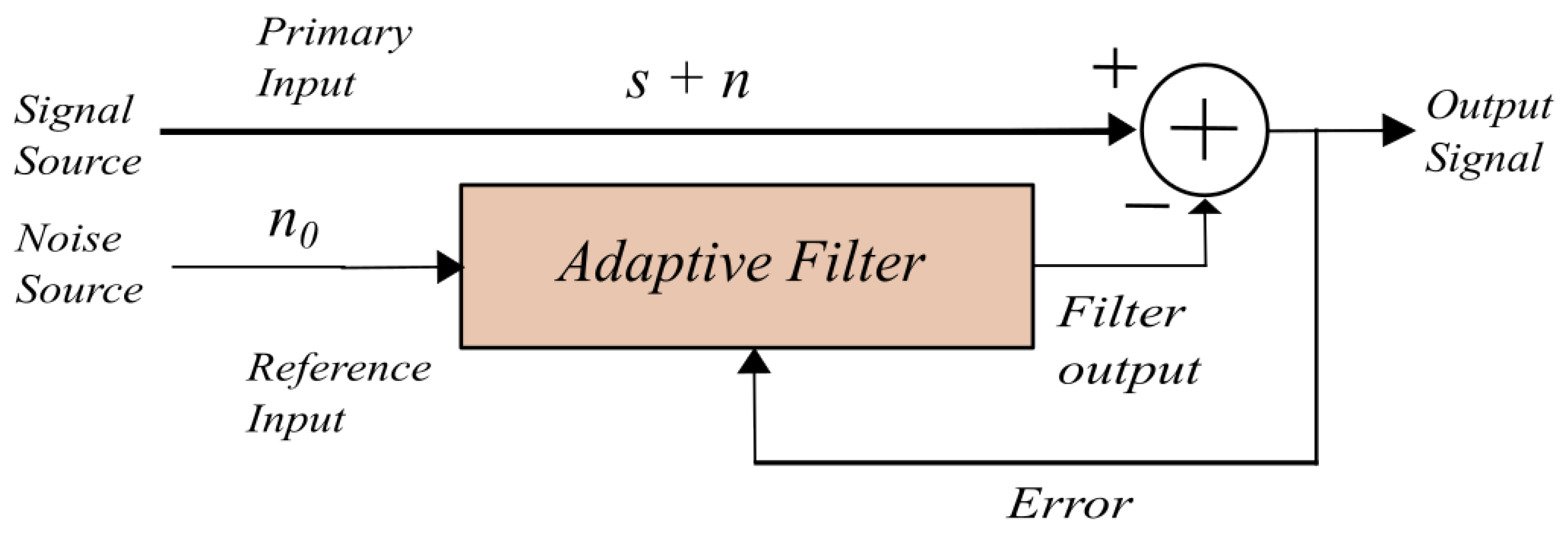
2.1. Least Mean Squares (LMS) Algorithm

The Least Mean Squares (LMS) algorithm is a good approximation of the steepest descent procedure. A significant feature of LMS is its simplicity, as it does not require the measurement of the pertinent correlation functions or matrix inversion, as is the case in the Steepest Descent Method (SDM). The initial weight vector of the filter is set as a zero vector, represented as follows:

The weight vector: $w\left(k\right)=[w_0\left(k\right),w_l\left(k\right),w_2\left(k\right),\cdots ,w_I\left(k\right)]$ where: $W_{initial}=w\left(0\right)$. The LMS algorithm is then applied as follows: For all values of k,

• The filter output is calculated as: $y\left(k\right)=w^T\left(k\right)x\left(k\right)$;
• Calculate the error signal: $e\left(k\right)=d\left(k\right)-y\left(k\right)$;
• Update filter coefficients and repeat procedure: $w(n+1)=w\left(n\right)+\mu x\left(k\right)e\left(k\right)$.

Here, $\mu$ is the step size that determines the convergence speed of the algorithm and w is the weight vector of the filter. The learning curve J can be obtained by $J=e^2\left(k\right)$ [24]. For the derivation of the Steepest Descent Method, please refer to Appendix B. A male voice signal was recorded using a microphone in a Record Studio, where noise is practically negligible, the signal was passed through a digital audio interface. Then, the resulting STEM wave file was processed in MATLAB. A Gaussian noise was added and the resulting corrupted signal then filtered using the LMS algorithm and SDM [25,26,27,28]. For the MATLAB script for the implementation of the LMS algorithm refer to Appendix C. Figure 2 shows the full LMS process.

By the way, we are aware that in certain applications, like telecom echo cancellation, LMS filters are adapted to the channel to cancel out noise. However, in our study, since we are dealing with a noise signal that is not pre-known, the LMS filter adapts to the noise characteristics in an attempt to reduce its impact on the signal rather than canceling it out completely.

2.2. Signal Processing

Signal processing was performed using the Least Mean Squares (LMS) algorithm implemented in MATLAB. The algorithm was applied to a male voice recording that had been corrupted with Gaussian noise, resulting in a signal with a degraded Signal-to-Noise Ratio, corrupted signal SNR was 10 dB. The noise reduction achieved by the LMS filter improved the SNR by 20 dB (for the detailed equation used to calculate the SNR improvement, please refer to the appendix). To visualize the effects of the noise reduction, the Fast Fourier Transform (FFT) of both the corrupted signal and the filtered signal were computed.

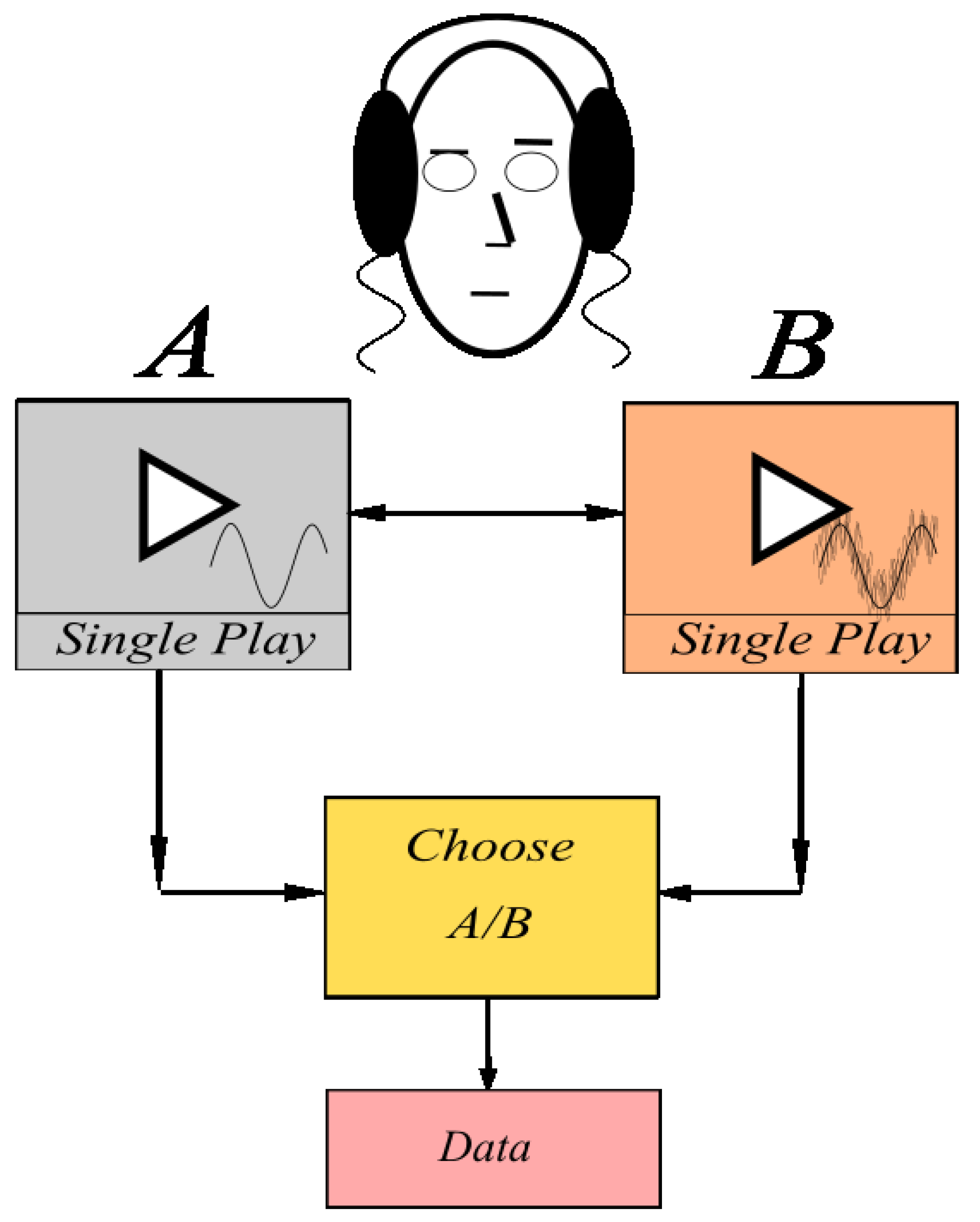
2.3. Blind Test Design

To assess the effectiveness of the LMS filter on human perception, a blind test was designed. A total of 30 young adult participants, aged between 20 and 30 years, were recruited for the study. Each participant was provided with a pair of earphones and a mobile phone to listen to the audio signals. They were presented with two signals, labeled A and B, and were asked to identify which signal had undergone noise reduction. The order of presentation was randomized, and participants were unaware of which signal was the filtered version, ensuring the integrity of the blind test. Their responses were recorded for later analysis. The test was conducted in a controlled environment inside a soundproof recording booth to prevent external noise interference. This setting ensured that the only noise present was the Gaussian noise initially introduced into the signal. A schematic of the experimental setup is presented in Figure 3, detailing the experiment design.

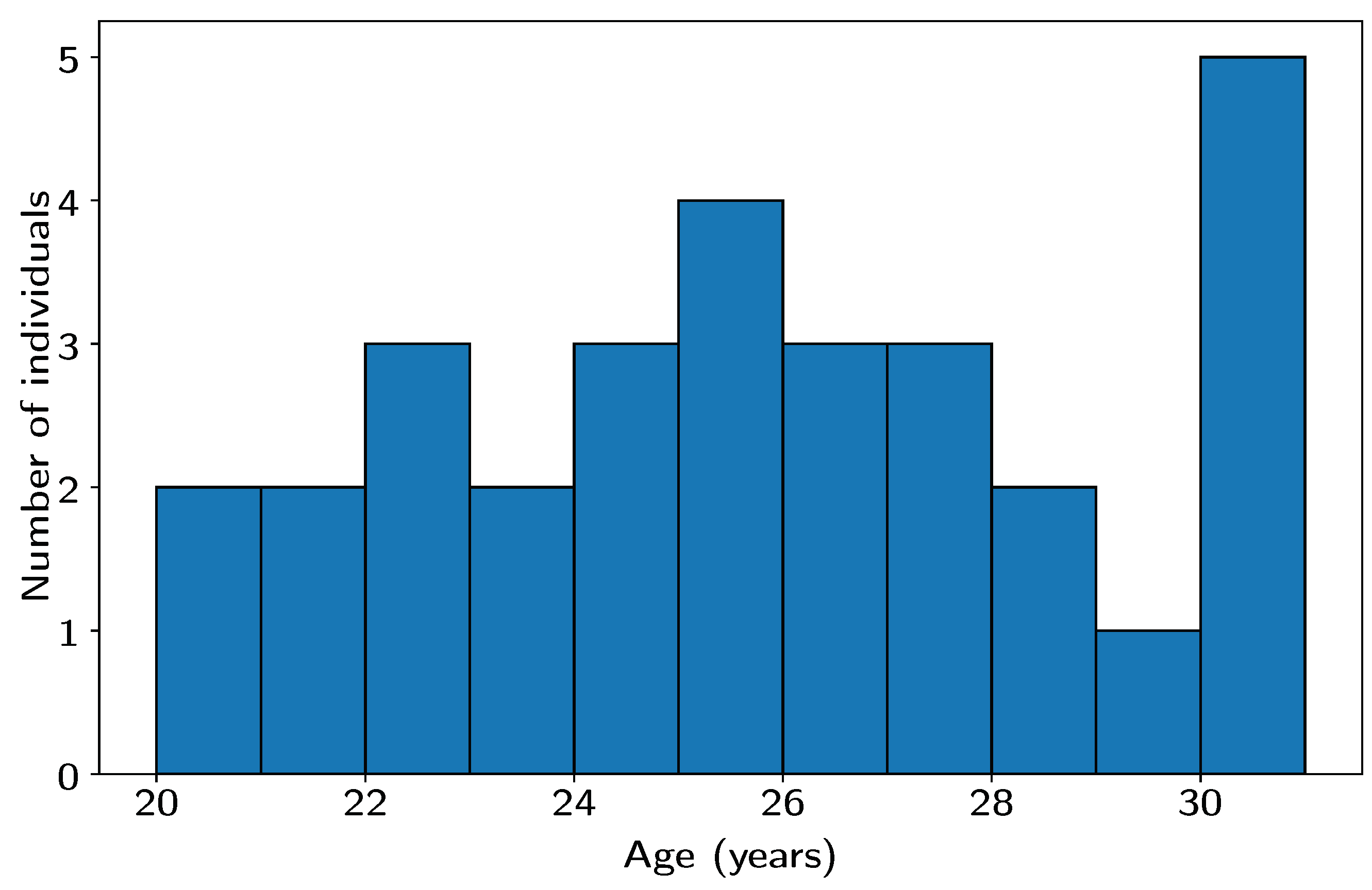
2.4. Data Collection

The responses of the participants were categorized into two options: “A” for the noise-reduced signal and “B” for the noise-corrupted signal. The frequency of correct and incorrect identification was recorded for each participant. The results were then compiled and analyzed to assess the overall effectiveness of the LMS filter in improving the perception of the signal. For all collected data refer to Appendix A.

2.5. Statistical Analysis

The data obtained from the blind test were analyzed using a Z-test for proportions to make statistical inferences regarding the effectiveness of the noise reduction. This test was applied to compare the proportion of correct identifications of the filtered signal with the proportion expected by chance (50%). A significance level of 0.05 was used to determine whether the LMS filter produced a statistically significant improvement in the participants’ ability to correctly identify the noise-reduced signal. In this study, the effectiveness of the LMS filter in improving the perception of the noise-reduced signal was analyzed using a Z-test for proportions. The Z test for proportions is a statistical test that determines if there is enough evidence to support a claim about a process, used to determine whether the proportion of correct identifications is significantly different from the proportion hypothesized of 50% (i.e., random guessing in the absence of noise reduction). The null hypothesis ($H_0$) states that the proportion of correct identifications is equal to the hypothesized value, while the alternative hypothesis ($H_1$) posits that the proportion is greater than the hypothesized value [29] (i.e., the LMS filter improves the perception of the signal).

• Hypotheses:

Null Hypothesis ($H_0$):

The proportion of correct identifications, p, is equal to 0.5 (i.e., no improvement, random guessing).

Alternative Hypothesis ($H_1$):

The proportion of correct identifications, p, is greater than 0.5 (i.e., the filter improves the perception). The Z-test statistic for proportions is calculated using the following formula:

$$Z={\displaystyle \frac{p_{\mathrm{observed}}-p_0}{\sqrt{\frac{p_0(1-p_0)}{n}}}}$$

where:

$p_{\mathrm{observed}}$ is the observed proportion of correct identifications.

$p_0$ is the hypothesized proportion (0.5 for random guessing).

n is the sample size or number of participants (30 in the case of this study).

2.6. Confidence Interval

In addition to the Z-test, the 95% confidence interval for the true proportion of correct identifications is calculated to provide a range of plausible values for the population proportion. This confidence interval is given by the following equation:

$$CI=p_{\mathrm{observed} + -Z_{\alpha /2}}·\sqrt{{\displaystyle \frac{p_{\mathrm{observed}}(1-p_{\mathrm{observed}})}{n}}}$$

$CI$ is the confidence interval for the proportion.

$p_{\mathrm{observed}}$ is the observed proportion of correct identifications.

$Z_{\alpha /2}$ is the Z-value for a 95% confidence level (typically 1.96) [29].

n is the sample size (30 participants in this study). If the calculated Z-value exceeds the critical value (1.96 for a 95% confidence level), the null hypothesis is rejected, indicating that the LMS filter significantly improved the perception of the signal. The confidence interval provides an estimate of the range in which the true proportion of correct identifications is likely to fall, with 95% certainty.

3. Results

Figure 4 presents a comparison between the time-domain signals and the filter’s response. However, due to the complexity of time-domain analysis, it is more effective to examine the system’s frequency response using the Fast Fourier Transform (FFT) of both the noise-corrupted and desired signals. The FFT results are shown in Figure 5, where a significant reduction in noise is observed, particularly within the frequency range most sensitive to the human ear (3–5 kHz). Figure 5 further illustrates the attenuation of Gaussian random noise across the 1 kHz to 10 kHz range. A noise attenuation of 20 dB in terms of SNR was achieved, with a step size of $\mu =0.01$. Figure 6 shows the distribution of data obtained from the Blind Test, categorized by participant age and their ability to correctly identify the filtered signal compared to the noise-corrupted one (choices A and B). In the experiment, each participant was given only one opportunity to listen to each signal, thus eliminating any potential bias from repetition. The experimental results indicated that, overall, 80% of the participants correctly selected the filtered signal, reflecting a high success rate in identifying the enhanced signal. However, an interesting trend emerged among the older participants (closer to 30 years of age), who exhibited a higher error rate compared to younger participants. This finding suggests that, despite the improvement in SNR provided by the LMS algorithm, factors such as age could influence the ability to correctly identify the signal, possibly due to differences in auditory perception or adaptation to signal processing technologies. Figure 7 illustrates the proportion of correct responses across all participants, highlighting the high rate of correct selections but also emphasizing the variation in performance based on age. Finally, Figure 8 presents the frequency distribution of participants ages, who were randomly selected within the 20 to 30 year-old range. This age range allowed for an equitable examination of the potential relationship between age and performance on the test.

3.1. Statistical Analysis and Interpretation

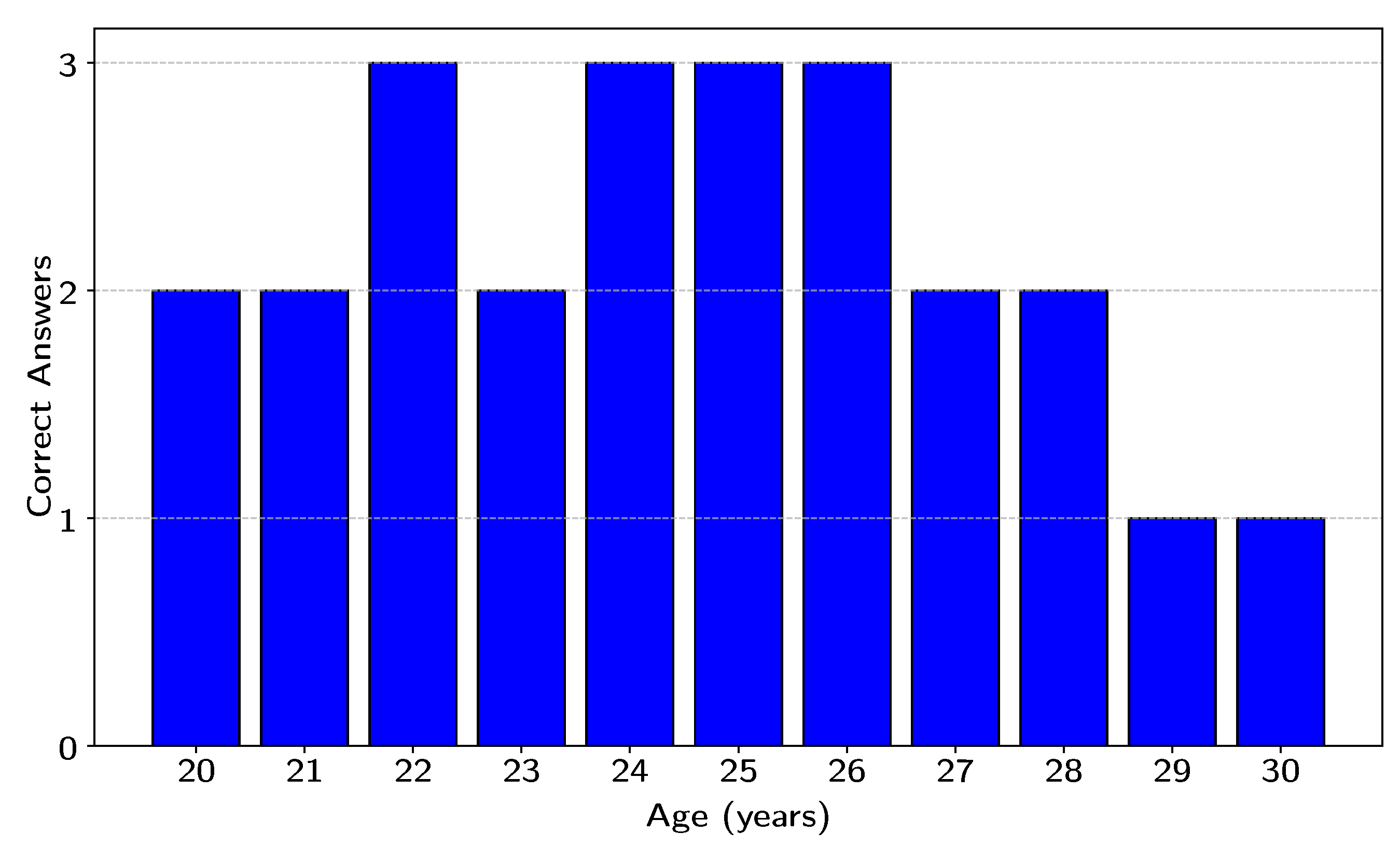
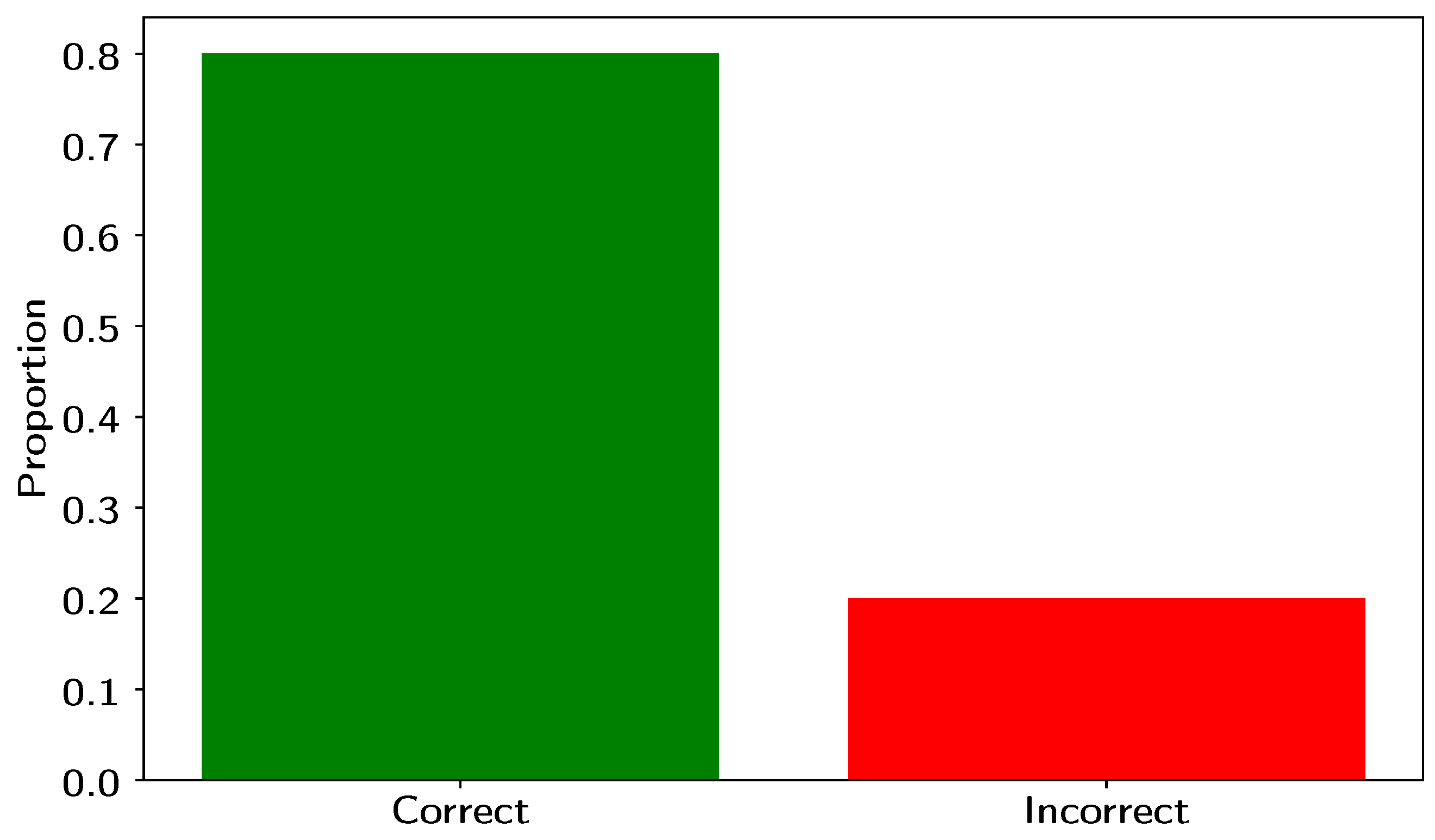
A Z-test for proportions was conducted to assess the effectiveness of the LMS filter in enhancing the ability of participants to correctly identify the filtered signal as compared to the corrupted signal. The test was designed to determine whether the proportion of correct responses, observed in the experiment, was significantly greater than what would be expected by random guessing.

3.2. Test Results

Observed proportion of correct answers: $\widehat{p}=0.8000$.

95% confidence interval: (0.6569, 0.9431).

3.3. Statistical Significance

The null hypothesis ($H_0$) posited that the observed proportion of correct responses is equal to 0.5, representing random guessing. This can be expressed as follows:

$$H_0:p_0=0.5$$

The alternative hypothesis ($H_1$) stated that the observed proportion is greater than 0.5, implying that the LMS filter had a significant effect on improving the perception of the filtered signal:

$$H_1:p>0.5$$

The test statistic for the Z -test is calculated using the following formula:

$$Z={\displaystyle \frac{p_{\mathrm{observed}}-p_0}{\sqrt{\frac{p_0(1-p_0)}{n}}}}={\displaystyle \frac{0.8000-0.5}{\sqrt{\frac{0.5(1-0.5)}{30}}}}=4.107$$

The resulting Z-value of 4.1079 is much greater than the critical value for a 95% confidence level (which is approximately 1.96), indicating that the null hypothesis can be rejected.The p-value associated with this Z-value is $p=0.0001$, which is far below the standard significance level of 0.05. Therefore, we reject the null hypothesis and conclude that the observed proportion of correct responses is significantly greater than what would be expected by random chance.

3.4. Confidence Interval

The 95% confidence interval for the true proportion of correct responses was calculated as (0.6569, 0.9431).This interval does not include 0.5, further supporting the conclusion that the proportion of correct responses is significantly higher than expected by chance. This suggests that the LMS filter had a positive effect on the ability of participants to distinguish the filtered signal from the noisy one.

4. Discussion

Figure 7 emphasizes the effectiveness of the LMS filter, while also suggesting the need for further investigation into age as a factor in the perception of filtered signals. The spectral plot clearly demonstrates a significant reduction in noise across the frequency spectrum, which serves as a preliminary indicator for evaluating the filter’s effectiveness [30]. However, it is important to acknowledge that this analysis does not yet fully capture the auditory response to the noise reduction in the signal. Unlike physical or objective quantities like sound level or intensity, loudness is a subjective interpretation of the listener. In the case of noise levels, even if two sounds have the same measured SPL, a sound with a wider bandwidth may be perceived as much louder than a sound with a smaller bandwidth. Additionally, the relationship between sound level and loudness is complex, as loudness is influenced by frequency. For example, a tone at 40 dB SPL is not necessarily perceived as twice as loud as a tone at 20 dB SPL. Moreover, individual differences in loudness perception are significant. A listener with hearing loss in certain frequency ranges will perceive signals in those ranges to be quieter than a listener with normal hearing. The equal loudness contours indicate that human hearing is most sensitive around 4 kHz, which helps explain why higher (treble) and lower (bass) frequencies might seem reduced or absent when audio is played at low levels. These factors are essential when evaluating the perceptibility of noise reduction, as they significantly affect how listeners perceive both the signal’s clarity and the reduction in unwanted noise. An interesting pattern emerged when considering the age of the participants in the experiment. The data revealed that individuals aged 30 and above (6 out of 30 participants) had greater difficulty identifying the correctly filtered signal compared to younger participants. This finding aligns with existing research that suggests age-related hearing loss first affects the frequencies most sensitive to human hearing, particularly those in the 3–5 kHz range [31], and the time response shows a gating effect on the signal noise. As a result, older participants may struggle to detect improvements in noise reduction within these frequencies, which are crucial for speech intelligibility and clarity. These findings provide additional evidence that hearing sensitivity is a significant factor in perceiving the effectiveness of the LMS filter, particularly in age groups with declining hearing acuity. The statistical analysis further supports the effectiveness of the LMS filter. The proportion of correct responses (80%) was significantly higher than the 50% expected by random guessing. This statistically significant outcome confirms that the noise reduction achieved by the LMS filter was perceptually noticeable to a large majority of participants. Consequently, this provides validation for the practical application of the LMS filter in improving speech intelligibility and reducing noise in real-world conditions, especially for younger individuals with better hearing acuity.

5. Conclusions

A comprehensive evaluation using a Z-test to assess the effectiveness of an adaptive Least Mean Squares (LMS) filter driven by the Steepest Descent 2 Method (SDM) is presented in this research article. The human auditory system does not perceive sound uniformly across all frequencies, with its sensitivity peaking around 4 kHz. This sensitivity diminishes for both lower and higher frequencies, which require higher sound pressure levels to be perceived as equally loud [14]. This foundational understanding of loudness perception plays a crucial role in designing audio systems that faithfully reproduce sound, especially in environments where background noise is prevalent. The variation in human hearing sensitivity across frequencies must be taken into account when developing technologies aimed at improving the auditory experience [8,32]. The LMS (Least Mean Squares) filter, implemented in this study, has shown remarkable efficacy in reducing noise and enhancing the clarity of the original signal. Specifically, the filter achieved a significant improvement (based on statistical results) in the Signal-to-Noise Ratio (SNR), with a noise reduction of 20 dB. These results provide evidence that the LMS filter is effective at mitigating noise interference and improving the perceptual quality of signals in environments where background noise poses a challenge. By adapting to the noise characteristics, the LMS filter minimizes the unwanted components, offering a cleaner and more intelligible signal [33,34]. Given the complexities of human hearing and the variability in perceptual responses among individuals, particularly across specific frequency bands, combining psychoacoustic principles with advanced noise reduction techniques like the LMS filter presents a powerful approach for improving audio experiences. The results underscore the importance of considering both auditory perception and technical advancements in noise reduction, while the LMS filter has shown great promise in this study, particularly among subjects in the 20–30 age range, future research should aim to broaden the scope of the study. A larger and more diverse sample size, including a wider age range, would provide a more comprehensive understanding of the filter’s effectiveness across different demographic groups [35,36]. The current study has demonstrated significant noise reduction in the target age group, but it is essential to explore how older individuals with varying degrees of hearing sensitivity (such as those above 30 years of age) might respond to the LMS filter [37]. This would offer more insights into the filter’s applicability across the population. Furthermore, future studies could focus on enhancing the LMS filter’s performance by improving its convergence speed and overall efficiency. Advances in algorithm optimization, such as adaptive step-size techniques or incorporating more sophisticated filtering methods, could lead to faster convergence while maintaining the quality of noise reduction. By refining the LMS algorithm and increasing its speed, it may be possible to achieve real-time processing for live audio applications, making it more practical for use in dynamic environments. It would be valuable to conduct long-term studies that assess the filter’s performance over extended periods of use, as this would help determine if the filter’s benefits persist over time and under varying environmental conditions. Investigating the filter’s robustness in different acoustic settings, such as in environments with fluctuating noise levels, could also provide critical insights into its potential for widespread application. The current study offers promising results for the application of the LMS filter in noise reduction and signal enhancement. Given the statistically significant results for the younger demographic (20–30 years), it is clear that the LMS filter represents a viable solution for improving perceptual audio quality in noisy environments. However, further studies are needed to explore its effects across a broader population and to enhance its performance, ensuring that it can be effectively applied across various use cases and listener groups. Additionally, a larger sample size is required to draw statistically reliable conclusions regarding the relationship between age and the effectiveness of the LMS filter. This limitation will be examined in future works.

References

1. Agnew, J. Audible circuit noise in hearing aid amplifiers. J. Acoust. Soc. Am. 1997, 102, 2793–2799. [Google Scholar] [CrossRef] [PubMed]
2. Keizer, G. The Unwanted Sound of Everything We Want: A book About Noise; PublicAffairs: New York, NY, USA, 2010. [Google Scholar]
3. Kim, S.; Arzac, S.; Dokic, N.; Donnelly, J.; Genser, N.; Nortwich, K.; Rooney, A. Cortical and Subjective Measures of Individual Noise Tolerance Predict Hearing Outcomes with Varying Noise Reduction Strength. Appl. Sci. 2024, 14, 6892. [Google Scholar] [CrossRef]
4. Ding, T.; Yan, A.; Liu, K. What is noise-induced hearing loss? Br. J. Hosp. Med. 2019, 80, 525–529. [Google Scholar] [CrossRef]
5. Mueller, B.J.; Liebl, A.; Herget, N.; Kohler, D.; Leistner, P. Using active noise-cancelling headphones in open-plan offices: No influence on cognitive performance but improvement of perceived privacy and acoustic environment. Front. Built Environ. 2022, 8, 962462. [Google Scholar] [CrossRef]
6. Alvarsson, J.J.; Wiens, S.; Nilsson, M.E. Stress recovery during exposure to nature sound and environmental noise. Int. J. Environ. Res. Public Health 2010, 7, 1036–1046. [Google Scholar] [CrossRef]
7. Münzel, T.; Sørensen, M.; Schmidt, F.; Schmidt, E.; Steven, S.; Kröller-Schön, S.; Daiber, A. The adverse effects of environmental noise exposure on oxidative stress and cardiovascular risk. Antioxid. Redox Signal. 2018, 28, 873–908. [Google Scholar] [CrossRef] [PubMed]
8. Frühholz, S.; Belin, P. The Science of Voice Perception; Oxford University Press: Oxford, UK, 2018; Volume 1. [Google Scholar]
9. Wang, X.; Xu, L. Speech perception in noise: Masking and unmasking. J. Otol. 2021, 16, 109–119. [Google Scholar] [CrossRef] [PubMed]
10. Masullo, M.; Yamauchi, K.; Dan, M.; Cioffi, F.; Maffei, L. Influence of Infotainment-System Audio Cues on the Sound Quality Perception Onboard Electric Vehicles in the Presence of Air-Conditioning Noise. Acoustics 2024, 7, 1. [Google Scholar] [CrossRef]
11. Ballou, G. Handbook for Sound Engineers; Taylor & Francis: Abingdon, UK, 2013. [Google Scholar]
12. Cheng, H.L.; Han, J.Y.; Chu, Y.C.; Cheng, Y.F.; Lin, C.M.; Chiang, M.C.; Wu, S.L.; Lai, Y.H.; Liao, W.H. Evaluating the hearing screening effectiveness of active noise cancellation technology among young adults: A pilot study. J. Chin. Med Assoc. 2023, 86, 105–112. [Google Scholar] [CrossRef]
13. Zacharov, N.; Ramsgaard, J.; Le Ray, G.; Jørgensen, C.V. The multidimensional characterization of active noise cancelation headphone perception. In Proceedings of the 2010 Second International Workshop on Quality of Multimedia Experience (QoMEX), Trondheim, Norway, 21–23 June 2010; pp. 130–135. [Google Scholar]
14. Jurado, C.; Gallegos, P.; Gordillo, D.; Moore, B.C. The detailed shapes of equal-loudness-level contours at low frequencies. J. Acoust. Soc. Am. 2017, 142, 3821–3832. [Google Scholar] [CrossRef]
15. Rasetshwane, D.M.; Trevino, A.C.; Gombert, J.N.; Liebig-Trehearn, L.; Kopun, J.G.; Jesteadt, W.; Neely, S.T.; Gorga, M.P. Categorical loudness scaling and equal-loudness contours in listeners with normal hearing and hearing loss. J. Acoust. Soc. Am. 2015, 137, 1899–1913. [Google Scholar] [CrossRef] [PubMed]
16. Glasberg, B.R.; Moore, B.C. Prediction of absolute thresholds and equal-loudness contours using a modified loudness model. J. Acoust. Soc. Am. 2006, 120, 585–588. [Google Scholar] [CrossRef]
17. Motlagh Zadeh, L.; Silbert, N.H.; Sternasty, K.; Swanepoel, D.W.; Hunter, L.L.; Moore, D.R. Extended high-frequency hearing enhances speech perception in noise. Proc. Natl. Acad. Sci. USA 2019, 116, 23753–23759. [Google Scholar] [CrossRef]
18. Kreiman, J.; Gerratt, B.R. Perceptual interaction of the harmonic source and noise in voice. J. Acoust. Soc. Am. 2012, 131, 492–500. [Google Scholar] [CrossRef]
19. Titze, I.R.; Palaparthi, A. Vocal loudness variation with spectral slope. J. Speech, Lang. Hear. Res. 2020, 63, 74–82. [Google Scholar] [CrossRef] [PubMed]
20. Tait, B.L. Applied Fletcher-Munson curve algorithm for improved voice recognition. Int. J. Electron. Secur. Digit. Forensics 7 2012, 4, 178–186. [Google Scholar] [CrossRef]
21. Chen, Y.; Gu, Y.; Hero, A.O. Regularized least-mean-square algorithms. arXiv 2010, arXiv:1012.5066. [Google Scholar]
22. McKenzie, T.; Armstrong, C.; Ward, L.; Murphy, D.T.; Kearney, G. Predicting the colouration between binaural signals. Appl. Sci. 2022, 12, 2441. [Google Scholar] [CrossRef]
23. Ang, L.Y.L.; Koh, Y.K.; Lee, H.P. The performance of active noise-canceling headphones in different noise environments. Appl. Acoust. 2017, 122, 16–22. [Google Scholar] [CrossRef]
24. Hayes, M.H. Statistical Digital Signal Processing and Modeling; John Wiley & Sons: Hoboken, NJ, USA, 1996. [Google Scholar]
25. Lee, J.H.; Ooi, L.E.; Ko, Y.H.; Teoh, C.Y. Simulation for noise cancellation using LMS adaptive filter. In Proceedings of the IOP Conference Series: Materials Science and Engineering, Busan, Republic of Korea, 25–27 August 2017; IOP Publishing: Bristol, UK, 2017; Volume 211, p. 012003. [Google Scholar]
26. Ferdouse, L.; Akhter, N.; Nipa, T.H.; Jaigirdar, F.T. Simulation and performance analysis of adaptive filtering algorithms in noise cancellation. arXiv 2011, arXiv:1104.1962. [Google Scholar]
27. He, Y.; He, H.; Li, L.; Wu, Y.; Pan, H. The applications and simulation of adaptive filter in noise canceling. In Proceedings of the 2008 International Conference on Computer Science and Software Engineering, Wuhan, China, 12–14 December 2008; Volume 4, pp. 1–4. [Google Scholar]
28. Foley, J.; Boland, F. Comparison between steepest descent and LMS algorithms in adaptive filters. In IEE Proceedings F (Communications, Radar and Signal Processing); IET: London, UK, 1987; Volume 134, pp. 283–289. [Google Scholar]
29. Martag, V.L. ; Rosa, A C. Bioestadística; Editorial El Manual Moderno: Mexico City, Mexico, 2014. [Google Scholar]
30. Yoshizawa, T.; Hirobayashi, S.; Misawa, T. Noise reduction for periodic signals using high-resolution frequency analysis. EURASIP J. Audio Speech Music Process. 2011, 2011, 5. [Google Scholar] [CrossRef]
31. Suzuki, Y.; Takeshima, H.; Kurakata, K. Revision of ISO 226 “Normal Equal-Loudness-Level Contours” from 2003 to 2023 edition: The background and results. Acoust. Sci. Technol. 2024, 45, 1–8. [Google Scholar] [CrossRef]
32. Stevens, S. Calculation of the loudness of complex noise. J. Acoust. Soc. Am. 1956, 28, 807–832. [Google Scholar] [CrossRef]
33. Narayan, S.S.; Peterson, A. Frequency domain least-mean-square algorithm. Proc. IEEE 1981, 69, 124–126. [Google Scholar] [CrossRef]
34. Rao, H.I.; Farhang-Boroujeny, B. Fast LMS/Newton algorithms for stereophonic acoustic echo cancelation. IEEE Trans. Signal Process. 2009, 57, 2919–2930. [Google Scholar] [CrossRef]
35. Carlile, S.; Hyams, S.; Delaney, S. Systematic distortions of auditory space perception following prolonged exposure to broadband noise. J. Acoust. Soc. Am. 2001, 110, 416–424. [Google Scholar] [CrossRef]
36. Srivastava, D.; Narayanan, V.; Singh, B.; Verma, A. A Novel Steepest Descent Least Mean Square Control for Smooth Mode Transfer of a Single-Stage SPVA-BES Hybrid Microgrid. IEEE Trans. Ind. Appl. 2024, 60, 7250–7263. [Google Scholar] [CrossRef]
37. Schäffer, B.; Pieren, R.; Schlittmeier, S.J.; Brink, M. Effects of different spectral shapes and amplitude modulation of broadband noise on annoyance reactions in a controlled listening experiment. Int. J. Environ. Res. Public Health 2018, 15, 1029. [Google Scholar] [CrossRef]
Figure 1. Adaptive filter algorithm diagram.
Acoustics 07 00020 g001
Figure 2. Full LMS filter process of the signal.
Acoustics 07 00020 g002
Figure 3. Representation of the blind test design and data generation.
Acoustics 07 00020 g003
Figure 4. (a) Audio signal corrupted by Gaussian Noise. (b) Filtered Audio signal.
Acoustics 07 00020 g004
Figure 5. (a) FFT of Audio signal corrupted by Gaussian noise. (b) FFT of filtered audio signal.
Acoustics 07 00020 g005
Figure 6. Bar plot of data obtained from the blind test, categorized by participant age.
Acoustics 07 00020 g006
Figure 7. Proportion of correct answers of individuals.
Acoustics 07 00020 g007
Figure 8. Bar plot of age distribution of the sample.
Acoustics 07 00020 g008
Disclaimer/Publisher’s Note: The statements, opinions and data contained in all publications are solely those of the individual author(s) and contributor(s) and not of MDPI and/or the editor(s). MDPI and/or the editor(s) disclaim responsibility for any injury to people or property resulting from any ideas, methods, instructions or products referred to in the content.