Abstract
The sonoscape of a small town at the foot of the Northern Apennines Mountains in north–central Italy was studied using a regular grid of automatic recording devices, which collected ambient sounds during the spring of 2024. The study area is characterized by high landscape heterogeneity, a result of widespread suburban agricultural abandonment and urban development. Sonic data were analyzed using the Sonic Heterogeneity Index and nine derivative metrics. The sonic signatures from 26 stations exhibited distinct, spatially explicit patterns that were hypothesized to be related to a set of 11 landcover types and seven landscape metrics. The unique sound profile of each sample site was consistent with the emerging heterogeneity of landcover typical of many Mediterranean regions. Some sonic indices exhibited stronger correlations with landscape metrics than others. In particular, the Effective Number of Frequency Bins Ratio (ENFBr) and Sheldon’s Evenness (E) proved particularly effective at revealing the link between sonic processes and landscape patterns. The sonoscape and landscape displayed correlations significantly aligned with their variability, highlighting the ecological heterogeneity of the sonic and physical domains in the study area. This case study underscores the importance of selecting appropriate metrics to describe complex ecological processes, such as the relationships and cause-and-effect dynamics of environmental sounds among human altered landscapes.
1. Introduction
In urban landscapes, the challenges of conserving biodiversity and naturalness while accommodating the living conditions and needs of human inhabitants are critical issues. Ecosystems have become more fragile with the continued and relentless expansion of urban areas, the increase in impervious surfaces, habitat fragmentation, and the gradual loss of natural areas. These actions have also led to an increase in species extinctions at local and global scales [1,2]. Industrialized anthropogenic phenomena inevitably reduce the complexity of natural cycles with results that are often underestimated in terms of their impact to ecosystem resiliency.
For decades, the Mediterranean region has experienced the gradual abandonment of rural areas and the depopulation of villages [3,4], leading to profound changes in both rural and urban landscapes. Such changes in human land use have had significant impacts on plant and animal communities, notably altering their composition and structure. These physical changes coincide with significant shifts in the patterns and processes of the sonic environment that exists in every landscape [5]. The subsequent fragmentation caused by human activities is expected to be reflected in the sonic mosaic, creating new dynamic sonic fields that interact with the physical landscape. For this reason, an ecoacoustic approach to understanding ecological processes and their response to human-altered environments becomes an important analytical and interpretative tool that provides a more inclusive ecological perspective to human–environmental relationships [5,6].
Ecoacoustics has found applications across many research and management fields, including biodiversity monitoring [7], urban ecology [8], conservation biology [6], environmental impact assessment [9], climate change studies [10,11], aquatic ecosystems [12], agroecology, public health and well-being [13], as well as education and public awareness [14]. In urban environments undergoing significant surface development, Ecoacoustics plays a crucial role in monitoring changes within local communities of soniferous species (e.g., insects, amphibians, mammals, and birds [12,15]) and geophysical and human activities [16]. This additional knowledge, in turn, enhances the understanding of ecological dynamics, aiding humans in selecting the most effective strategies to conserve biodiversity, address noise, and create better living conditions for people.
Human developments and quality of life have been linked to the effects of climate change, and many ecosystems are also under significant stress and ecological crises [17]. Because rural areas affected by human development are among the least resilient ecosystems [18], and Mediterranean landscapes represent an interesting example of human land use, we set out to investigate the relationship between the sonoscape and a heterogeneous landscape along a rural–urban interface in north–central Italy. By applying the systems-based approach of Ecoacoustics, we expected our findings would provide a unique and more holistic interpretation of this effected landscape as a case study on the ecological dynamics of a common rural–urban village in southern Europe [19]. As such, an ecoacoustic approach makes climate adaptation and resilience more achievable [20]. By embracing the perspectives of the physical and sonic domains, this approach may provide land managers and city planners in these village types an effective pathway to assessing environmental complexity, taxonomical variety, and ecological diversity to identify desired conditions.
Our objectives were to:
- (1)
- Assess the current conditions of the sonoscape that emerged from a small urban town set within a rural Mediterranean landscape, which has experienced moderate urban development outside its historic center and a simultaneous abandonment of the adjacent rural landscape.
- (2)
- Determine the composition, complexity, and spatio-temporal composition of geophonies, biophonies, and technophonies as indicators of geophysical, biological, and anthropogenic processes that play out in this urban–rural landscape.
- (3)
- Identify the relationship between these sonic components and the spatial and structural characteristics of landcover types across the urban–rural interface combining ecoacoustic indices and landscape metrics.
2. Materials and Methods
2.1. Study Area
2.1.1. Geographical Profile
The town of Fivizzano (Massa-Carrara Province, Tuscany Region, Italy), municipal capital of the Fivizzano Commune, located at Latitude 44°14′ N, Longitude 10°07′ E, and 325 m ASL, lies along National Road No. 63, which connects the Tuscan-Ligurian Tyrrhenian coast to the Emilia-Romagna region crossing the Northern Apennines Mountains (source: Wikipedia, 2 October 2024).
Once an important mid-sized center, Fivizzano has lost much of its prominence in recent years, partly due to the construction of the A15 Parma-La Spezia highway—also known as the CISA truck route—in the 1970s, which, being 20 km away, significantly reduced vehicular traffic through the area. The town’s population is relatively stable (1500 inhabitants), but this number increases by 10% in the summer due to the influx of tourists attracted by the landscapes of the Tosco-Emiliano Apennines, the Apuane Alps, and the Cinque Terre coast. The historic center of Fivizzano extends in a NE–SW direction, covering an area of 1 km × 200 m. A residential area built after 1970 extends to the east with the same orientation as the historic center, covering an area of 700 × 250 m. The new developed area is separated from downtown by a small stream and by the bypass of National Road No. 63, which was built in the 1960s (Figure 1).
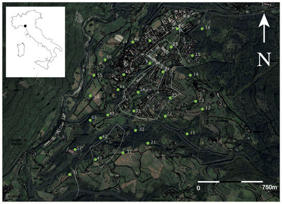
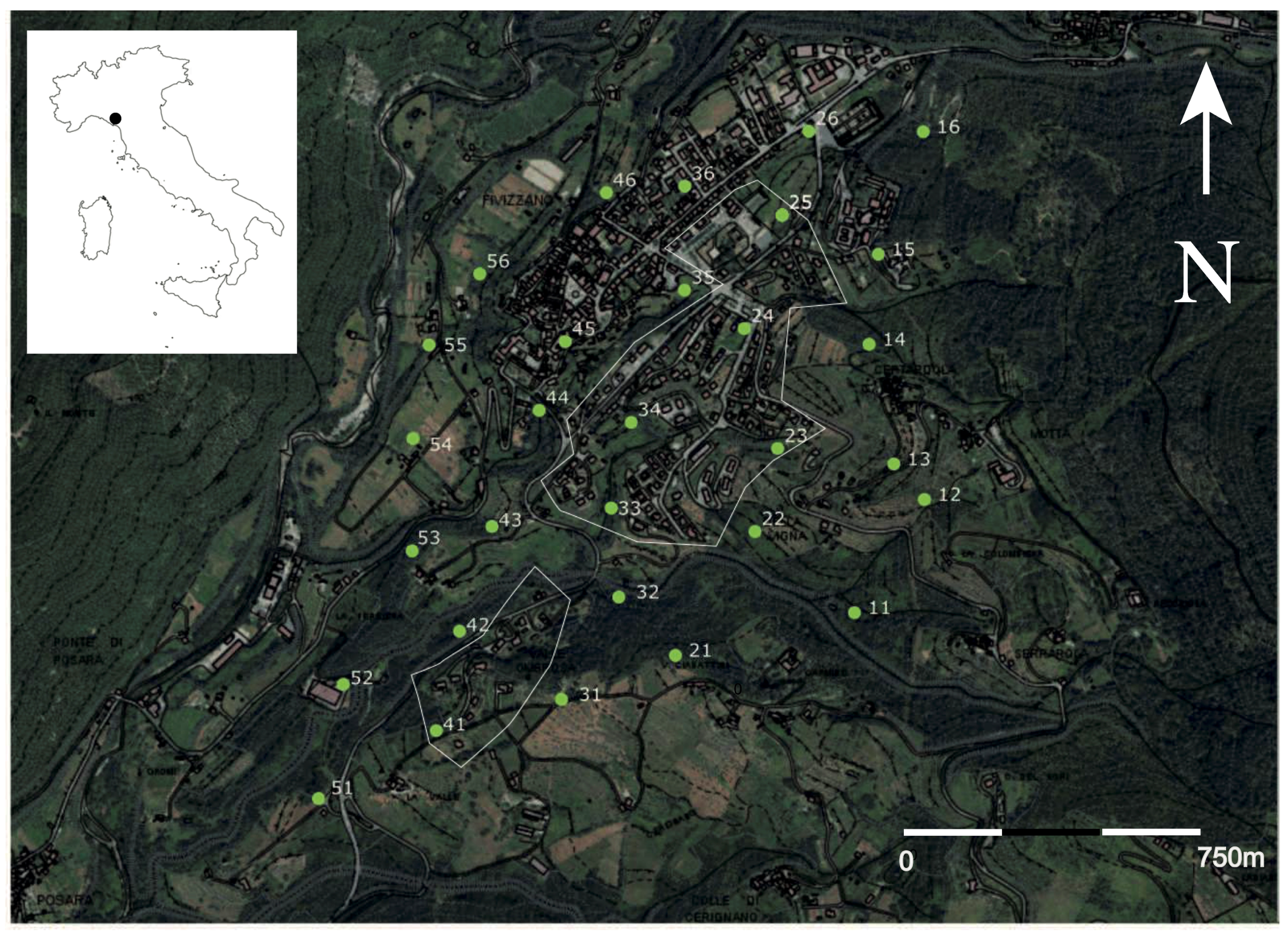
Figure 1.
Satellite image of the study area (Fivizzano, Massa-Carrara Province, Tuscany Region, Italy, 44°14′ N, 10°07′ E) showing the distribution of 30 recording stations. The regions enclosed by the white line represent areas of recent urban development.
2.1.2. Landscape Characters
The urban and rural landscapes of Fivizzano have undergone significant transformations that complicate its ecological characterization. Historically, distinct boundaries between the urban and surrounding rural areas were maintained, but these divisions have blurred over time. Two primary factors have contributed to this shift: (1) the widespread abandonment of agricultural practices and (2) the uncontrolled expansion of new housing developments beyond the original downtown.
The abandonment of agriculture has led to a loss of the rural structures and patterns that once defined the landscape, causing a reduction of the clear demarcation between urban and rural spaces. Meanwhile, the rapid and often unplanned construction of residential areas in previously rural zones has further disrupted the natural and cultural spatial order. Aerial imagery from 1954 (Figure S1) provides a clear illustration of this transformation, highlighting the extent to which the urban area of Fivizzano has expanded at the expense of traditional agricultural lands, which have either been reduced or abandoned. The contrast between the landscape of 1954 and the present underscores the dramatic changes in land use and urbanization, making it difficult to trace the historical boundaries of the landscape and the connections that once existed between the town and its surrounding rural areas.
2.1.3. Geological Characters
The settlement of Fivizzano extends over terraced alluvial soils composed of inactive alluvial deposits of silty gravels (a mixture of gravel, sand, and silt, with an abundant fine fraction). To the east, these deposits come into contact with the Oligocene–Miocene bedrock, with the Groppo del Vescovo limestones from the Eocene, and the Canetolo clays and limestones from the Paleocene–Eocene. To the west, the Rosaro stream marks the boundary of the study area and geologically demarcates the border with the Ottone-Monteverdi Flysch from the Upper Cretaceous. Figure S2 shows the geological map extracted from the portal of the Tuscany Region website (https://www.regione.toscana.it/-/geoscopio).
2.1.4. Climatic Characters
The study area is inside the subhumid zone according to Thornthwaite classification [21], with abundant rain (1000 mm), especially from November to February. In Table S1, it is reported the distribution of the major climatic parameters collected during the survey period. The temperature ranged from 0.84 °C (7 March 2024) to 30 °C (18 June 2024).
2.2. Sampling Design
To test certain aspects of ecoacoustics theory, we employed a regular grid of recorders, hypothesizing that landscape heterogeneity correlates with sonic properties, thereby creating regional sonoscapes composed of a mosaic of sonotopes [22]. Thirty recording stations (RSs) were deployed according to a regular grid layout, with stations spaced 200 m apart in 5 rows and 6 columns to cover the selected area (Figure 1). The distance of 200 m is considered reasonable to ensure the independence of the majority of the biophonic sources, as recently demonstrated in an experiment conducted by Yip et al. [23]. Each RS was labeled based on its position in the grid (e.g., 11, 12, …, 55, 56). In some cases, the placement of stations had to be adjusted by a few meters to avoid manmade features such as buildings and roads. The grid was oriented with the rows running from southwest to northeast and the columns running perpendicular to this direction.
2.3. Morphological and Landcover Characterizations
A detailed description of the area around each recording station (RS) was performed within a rectangle, covering a ground area of 71,604 m2. Morphological and landcover information was obtained from the ‘Carta Tecnica del Comune di Fivizzano (CTCF)’ (https://sct-ucml.ldpgis.it/fivizzano/cartobase) and from the Regione Toscana WMS 2023 orthophoto (https://www.regione.toscana.it/servizi-wms/-/asset_publisher/8xiR17oEWJ23/content/geoscopio).
The maximum, minimum, and average elevation of each RS map were obtained by averaging the elevation of eight points along the perimeter of the rectangle (four points distributed in the middle of each side and four at the vertices). The slope of the RS map, expressed in degrees, was calculated as the difference in elevation between the RS and the 8 perimeter points, as previously described, using the equation θ = arctan(rise/run). The orientation of each RS map was determined by estimating the prevailing orientation categories (N, S, E, W, NW, SW, NE, SE, Flat) for each of the four sections into which the rectangle was divided. Orientation variability was expressed as the number of different orientations, ranging from 1 to 4, in each sub-rectangle.
To better distinguish buildings and roads—often distorted due to image projection on maps or obscured by tree shadows—layers from the CTCF were superimposed onto the orthophoto map.
Following a detailed field survey and the supervised classification of the orthophoto, 11 landcover classes (LCCs) were tentatively identified as important features of the landscape and likely correlated to the sonic heterogeneity: Woodland, Shrubland, Uncultivated area, Cultivated area, Bamboo grove, Olive orchard, Vineyard, Edgerows, Buildings, Roads, and Other (Table S1).
Despite widespread land abandonment in both uncultivated and cultivated areas, a great variety of fruit trees can now be found, including apple, cherry, fig, apricot, pear, and plum, as well as exotic plants such as persimmons and Japanese medlar. These fruit trees are planted haphazardly, without any specific order, with the aim of providing a wide variety of fruit for family consumption. The mix of plants, often interspersed without a clear design, creates a disordered pattern in the landscape, reflecting the evolution of an agricultural system that has strayed from traditional farming practices. Residual chestnut orchards persist on the more humid slopes, though they are now overtaken by black locust trees and parasitized by ivy.
Due to the complexity of the Fivizzano landscape, landcover classification required supervised classification after defining user-specific classes to ensure better control. The classification of images obtained around each recording station was conducted using Fiji® software (2.14.0) [24] following these steps (Figure 2):
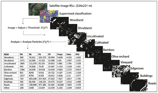
Figure 2.
Example based on the recording station RS56 of the procedures used to classify images. A supervised classification was obtained by applying the procedures from the Fiji software. The following parameters were considered: PN (Patch Number), PA (Patch Area), PS (Patch Size), PP (Patch Perimeter), Fmax (Maximum Feret Diameter), Fmin (Minimum Feret Diameter), and PFD (Patch Fractal Dimension).
Each original image of 324 × 221 m [2742 × 1864 pixels], with a resolution of 0.014 m, was resized to 1024 × 697 pixels, obtaining a soil resolution of 0.1 m using the Image > Scale tool to accelerate the classification process, as recommended, and to avoid computer crashes. The Trainable Weka Segmentation v.3.34, a Fiji plugin, was used to create a classifier with the ‘FastRandomForest model.’ The classifier was trained using more than 11 different land use categories that represented the majority of landcover types considered relevant for our investigation and potentially independent factors of the sonic variables. To verify the classifier’s robustness, it was iteratively trained over rounds using 10 different RS maps. Successively, every LCC image was split in the 11 landcover classes into a binary format using the following command sequence: Image > Adjust >Threshold.
Definitively, a specific folder was used for each image containing the classified image in 8-bit, and all eleven 8-binary images for each cover class, when present. Every separate LCC obtained with the previous procedures was submitted to a shape analysis using the command sequence Analyze > Analyze particles, obtaining landscape indices as described in Table 1.

Table 1.
The indices used to describe the structure and complexity of the landscape.
In addition, the Patch Fractal Dimension (PFD) for each of the eleven LCCs was obtained using the box counting method. This was accomplished by activating the command sequence Analyzing > Tools > Fractal Box Counting and setting the box sizes to 2, 3, 4, 6, 8, 12, 16, 32, and 64. The fractal dimension ranges from 0 (which corresponds to the dimension of a point) to 2, representing the dimension of an object that fills a 2D space (x, y) in a complex, but not fully complete, manner [29]. We expect a value close to 2 for a landscape feature developed in the xy plane, such as a landcover class (LCC), which exhibits a complex structure, filling the entire surface. Fractal analysis is commonly used to assess the complexity of landscape structures [30,31,32].
2.4. Methods for Collecting Sound Data
We deployed 30 automated recording units (SET™, Lunilettronik, 54013 Fivizzano, Italy) evenly distributed across our study area in a 5 × 6 grid, with an average spacing of 200 m between each SET. Recorders were mounted 1.2 m above the ground on tree trunks and positioned in a way that microphones (calibrated to 94 dbA) had an omnidirectional detection area. Recorders were programmed to sample the ambient sonic environment at a rate of 48,000 Hz with medium-high microphone gain (30). Recordings were scheduled to last 1 min, followed by a 5 min pause between recordings, continuously over a 24 h period, generating a total of 240 min of data per day in WAV audio format. Sampling took place from spring to summer, between 7 March and 3 July 2024, but only data from 1 April to 30 June were used for this analysis. Recordings were made over three sessions in (2, 13, 24) April and (5, 18, 29) May, and two sessions in (11 and 27) June. The last session in May included some days in June. Each session lasted 9 days; however, the first and last day of each session were not considered, using only the recordings from the 24 h periods.
2.5. Metrics Used to Process Sonic Data
2.5.1. Sonic Heterogeneity Indices (SHItf)
Sonic heterogeneity indices (SHItf), known also as Acoustic Complexity Indices [33], and some derivative metrics were utilized to process the FFT matrices obtained by WAV files using the SonoScape®1.1.0426 software [34]. An intensity filter of 0.01, to exclude nonenvironmental sounds, and clumping of 0 were applied. The SHItf are based on the Canberra distance metric [35,36] and operate on a fast Fourier transform (FFT) matrix. The SHItf calculate the difference in contiguous intensities of each frequency bin along a temporal interval, so that:
where SHItf is the total sonic heterogeneity of the ith frequency bin along a time interval j, xi,j and xi,j+1 are two contiguous values of intensity along a specific frequency bin i, and n is the number of temporal FFT intervals considered (typically segmented into 512 frequency bins separated every 46.875 Hz).
2.5.2. Spectral Sonic Signature (SSS)
The sonic signature refers to the sensed or interpreted sound sequences that characterize communities, locations, habitats, and ecosystems in the frequency or time domain [37].
The Spectral Sonic Signature (SSS) is obtained by averaging the total SHItf for each 512 frequency bins across all recording stations for the entire study area and describes graphically the frequential change in SHItf [34]:
2.5.3. Number of Frequency Bins (NFB)
The complexity encountered along an SSS can be represented by the Number of Frequency Bins (NFB), which, in our case, has a maximum value of 512. The greater the number of frequency bins present in a recording station (RS), the larger the contribution of sonic components. This index is straightforward and can be considered analogous to the measure of richness (i.e., the number of species) in an ecological community.
2.5.4. Spectral Variability (SV)
Spectral (sonic) variability (SV) is the attitude of a frequency category to assume different quantitative modalities [38]. It is calculated by applying the Gini–Simpson concentration index D to SHItf [38,39] as:
where n1 is the value of SHItf, and (where S is the number of frequency bins, and nl is the value of a frequency bin).
2.5.5. Effective Number of Frequency Bins (ENFB)
The Effective Number of Frequency Bins (ENFB) has been used to measure the complexity in the collection of frequency bins returned from the Gini–Simpson concentration index (D) [38,39]. It represents the effective number of equally common frequency bins necessary to produce the same heterogeneity as that observed in the sample [40]. Essentially, ENFB provides an index that reveals how sounds are effectively distributed and concentrated in the acoustic space [34].
We calculated ENFB as:
2.5.6. Effective Number of Frequency Bins Ratio (ENFBr)
We calculated ENFBr as
This index offers an alternative method to assess the internal complexity of the It reaches its maximum when the frequencies are evenly distributed across the different bins.
2.5.7. Spectral Sonic Evenness J′
This index is obtained by Pielou’s evenness (J′) [41]:
where H′ is the Shannon entropy [42] applied to the distribution of frequency bins, and S is the NFB.
J′ = H′/log S
2.5.8. Sheldon Index of Ecological Evenness (E)
This index has been obtained after a modification of the Sheldon index as proposed by Sheldon [43]:
where H′ is the Shannon–Wiener diversity index [42], and S = NFB [44,45,46]. This index is based on Hill’s diversity number [40].
2.5.9. Normalize Difference Sonic Index (NDSHI)
The original Normalize Difference Sonic Index (NDSI) [47,48] was based on a normalized value of power spectral density (watts/kHz), referred to as soundscape power, that occurs at 1 kHz frequency intervals within the frequency range of 1000–16,000 Hz for each sound recording. In our case, the index has been adapted, and instead of using the power spectral density, we used the SHItf. The index that we called NDSHI is calculated as the ratio of SHItf corresponding to frequency intervals commonly associated with technophony (0.2–2 kHz) and biophony (≥2 kHz).
2.5.10. The Alignment Between SSS and Landscape Variables
The dendextend package, the entanglement and cor.dendlist functions [49] operating in R [50], were used to visualize the alignment between the Spectral Sonic Signature and landscape variables in a dendrogram, with the degree of association measured by Goodman–Kruskal’s gamma coefficient (γ) [51,52]. The γ coefficient ranges between −1 and +1. The closer γ is to ±1, the stronger the positive or negative association, respectively. Conversely, the closer γ is to 0, the weaker the association, with 0 indicating no association. This analysis allowed us to determine whether the landscape variables measured at recording stations were associated with the complexity and concentration of sonic information distributed across frequency bins. The entanglement is a measure that ranges from 1 (full entanglement) to 0 (no entanglement).
JMP [53] statistical package (Student edition) has been utilized to perform the Cluster Analysis using the Ward methods and the Pearson Correlation index.
3. Results
3.1. Morphology and RS Landcover
The study area was characterized by elevations ranging from 260 to 436 m, with slopes varying from 5 to 11°, predominantly possessing a NW and W aspect followed by Flat and SW classes (Table S2). Of the 11 landcover classes, edgerows were the most common, followed by woodlands, paved roads, and uncultivated areas (Table 2).
Table 2.
Characterization of the landcover categories based on landscape indices obtained by averaging data from all the RS. PA: Patch Area, PN: Patch Number, PS: Patch Size, PP: Patch Perimeter, Fmax: Maximum Feret Patch Dimension, Fmin: Minimum Feret Patch Dimension, PFD: Patch Fractal Dimension.
Cluster analysis, based on the seven landscape indices (PA, PN, PS, PP, Fmax, Fmin, and PFD), excluding “roads”, “buildings”, and “other”, revealed an aggregation where woodlands, edgerows, and uncultivated areas represented the most distinct landcover categories. Shrublands and bamboo groves fell within the same cluster, while olive orchards and vineyards grouped together (Figure 3).
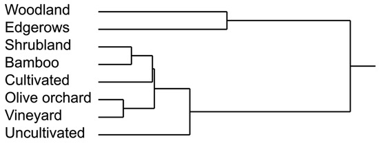
Figure 3.
Landcover clustering obtained according to seven landscape indices (PA, PN, PS, PP, Fmax, Fmin, and PFD). We have excluded from this classification “buildings”, “roads”, and “other” landcover categories.
Tentatively, 10 clusters were sufficient to aggregate sample sites into similar groups based on 11 landcover categories and seven landscape indices (Figure 4).
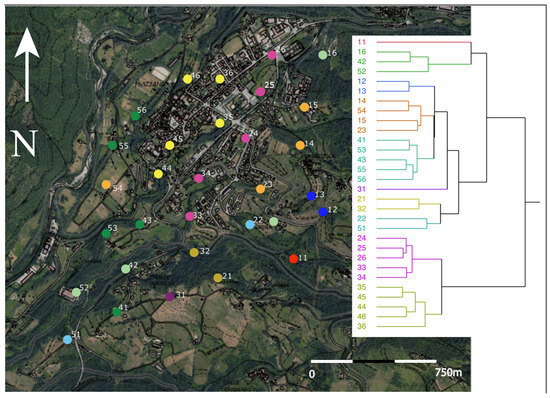
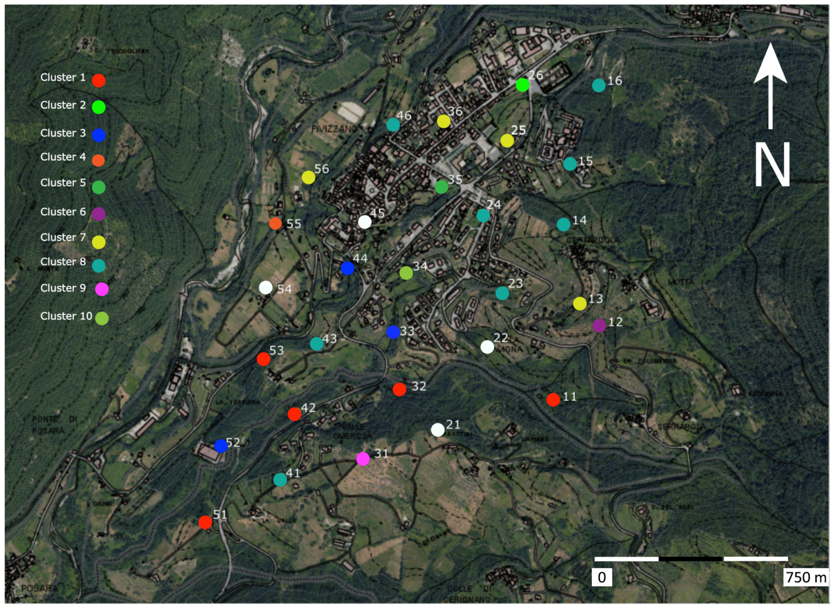
Figure 4.
Aggregation based on a 10-cluster model of the recording stations (RSs), according to the landscape characteristics of Table S3. Each cluster branch is marked with a different color, and the same colors are used in the maps to indicate the aggregation categories among the RS.
3.2. The Sonic Data
Table S4 shows the number of days recorded by each recording station (RS) over the entire period. Four of our SETs experienced malfunctions during certain periods, resulting in incomplete data sets, and were subsequently excluded from analysis. We acquired a total of 319,920 min of ambient sounds across 26 RSs that operated effectively from April to June 2024.
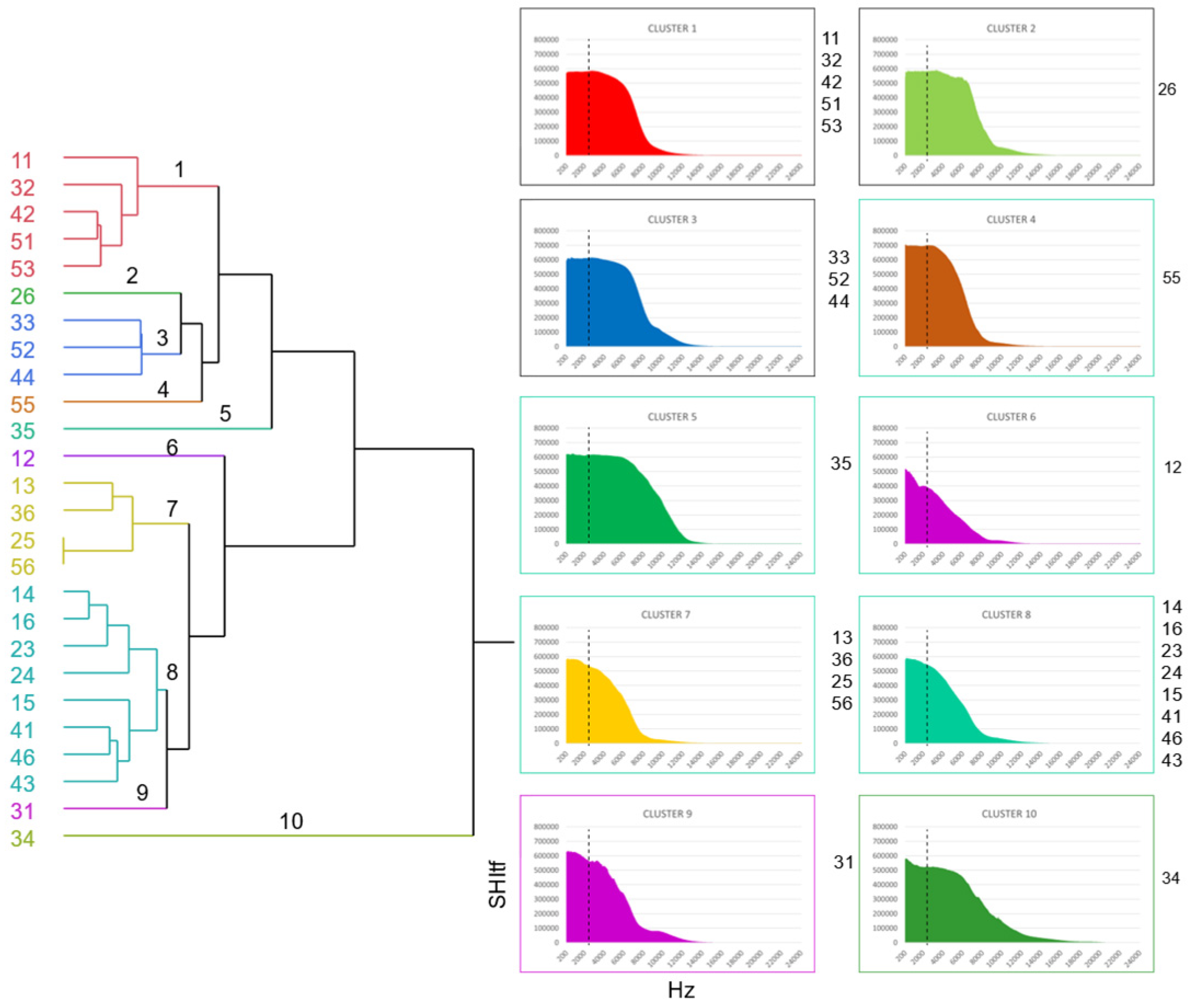
Figure S3 shows the sonic signatures of all 26 RSs averaged for each month of sampling (April, May, and June). Each RS had a distinct sonic signature that remained similar across all the three months. Cluster analysis of SHItf values across all months, assuming a 10-sonotope model, revealed spatially explicit patterns of sonic variation across the study area (Figure 5 and Figure 6). The largest, and most commonly shared sonic activities, were displayed in Cluster 8, with eight RSs, and Cluster 1, with five RSs. However, there were five RSs (RS55, RS35, RS12, RS34, and RS31) that were distinctively clustered separately from other RSs, suggesting these sample sites may have distinct sonic characteristics from others.
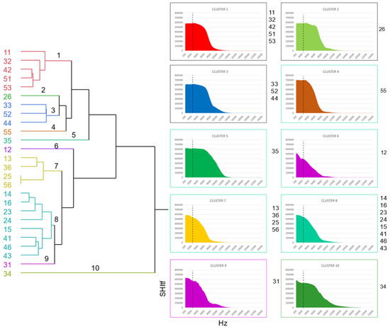
Figure 5.
Similarities between the acoustic signatures of each RS. Using a 10-sonotope model, it has been possible to distinguish RSs with unique sonic signatures (RS55, RS35, RS12, RS34, and RS31). The dashed line marks the boundary between potential geophonies and technophonies (<2000 Hz), and biophonies (≥2000 Hz). The RSs that belong to each of the 10 clusters are indicated alongside their respective sonic signatures.
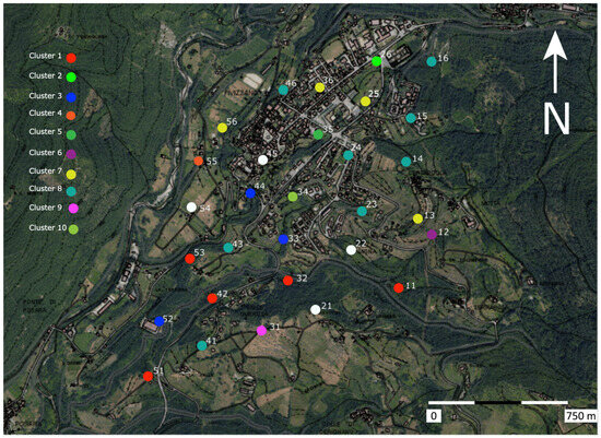
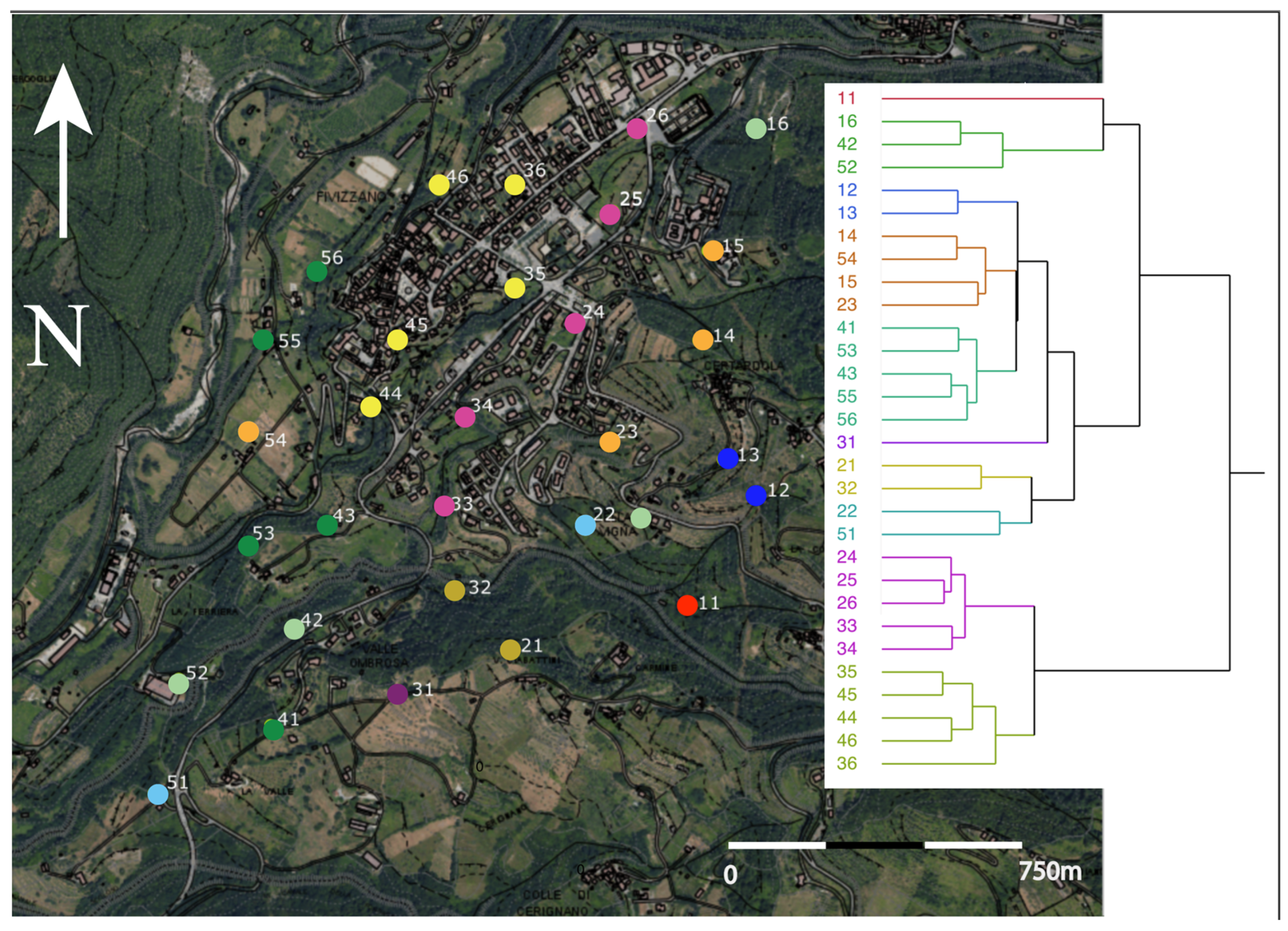
Figure 6.
Classification of the RSs based on cluster analysis applied to the sonic signatures from April to June. The RSs indicated by white spots have been excluded from the analysis due to malfunctioning or insufficient data. The color assigned to each RS corresponds to the color of the branches in the dendrogram of Figure 5.
Pursuant to our hypothesis that these distinct sonic arrangements are related to the physical landscape, we analyzed sonic patterns according to the generally known sonic distinctions between low-frequency technophonies and geophonies (SHItf < 2000 Hz), and mid-high-frequency biophonies (SHItf ≥ 2000 Hz) (Gage and Axel, 2014 [48]), allowing for a sub-grouping of sonic patterns across the landscape (Figure 7a,b). These separate frequency classifications of sounds facilitated a better understanding of the complex patterns in these soundscapes.
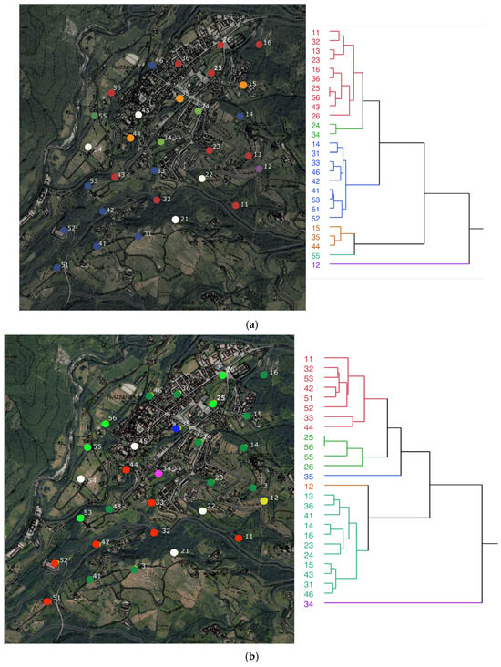
Figure 7.
(a) Cluster analysis applied only to SHItf < 2000 Hz. (b) Cluster analysis applied only to SHItf ≥ 2000 Hz.
Assuming a six-sonotope model restricted to the SHItf < 2000 Hz, RSs were predominantly grouped into two major clusters, represented in Figure 7a by the colors blue and red. This resulted in a clearly visible distinction in sonic distribution for sample sites, with similar low-frequency characteristics at the edges and outer periphery of the village likely associated with geophonic sources, while sites clustered in orange and light green were configured more generally near the village center more closely associated with technophonic sources (Figure 7a).
With a similar assumptive six-sonotope model SHItf ≥ 2000 Hz, sonic activity exhibited more complex spatial arrangements. Specifically, Cluster 1, indicated in Figure 7b as red, forms a linear sequence of RSs following a small stream. Conversely, the second largest cluster, indicated in Figure 7b as dark green, displayed three visually distinct and isolated groupings outside the village center. The next smallest cluster of sample sites, indicated in Figure 7b as light green, were distinctively clustered along the village’s outer western periphery, with an isolated spatial group located on the northern edge of town.
There was a strong correspondence between cluster groupings and the average SHItf among RSs, especially for frequencies < 2000 Hz, confirming that the separation of these two frequency ranges provided a valuable representation of sonic and spatial variability in the soundscape (Table 3).
Table 3.
Total SHItf sorted from lowest to highest for each RS, with frequencies <2000 and ≥2000 Hz. The cluster analysis was based on the 6-sonotope model.
The overall level of correspondence between environmental data (morphology + landcover) and the sonic signature of the study area possessed a Goodman–Kruskal’s gamma coefficient of 0.042. When separated according to low- and mid-high-frequency categories, the coefficients resulted in 0.041 for SHItf < 2000 Hz and 0.034 for SHItf ≥ 2000 Hz.
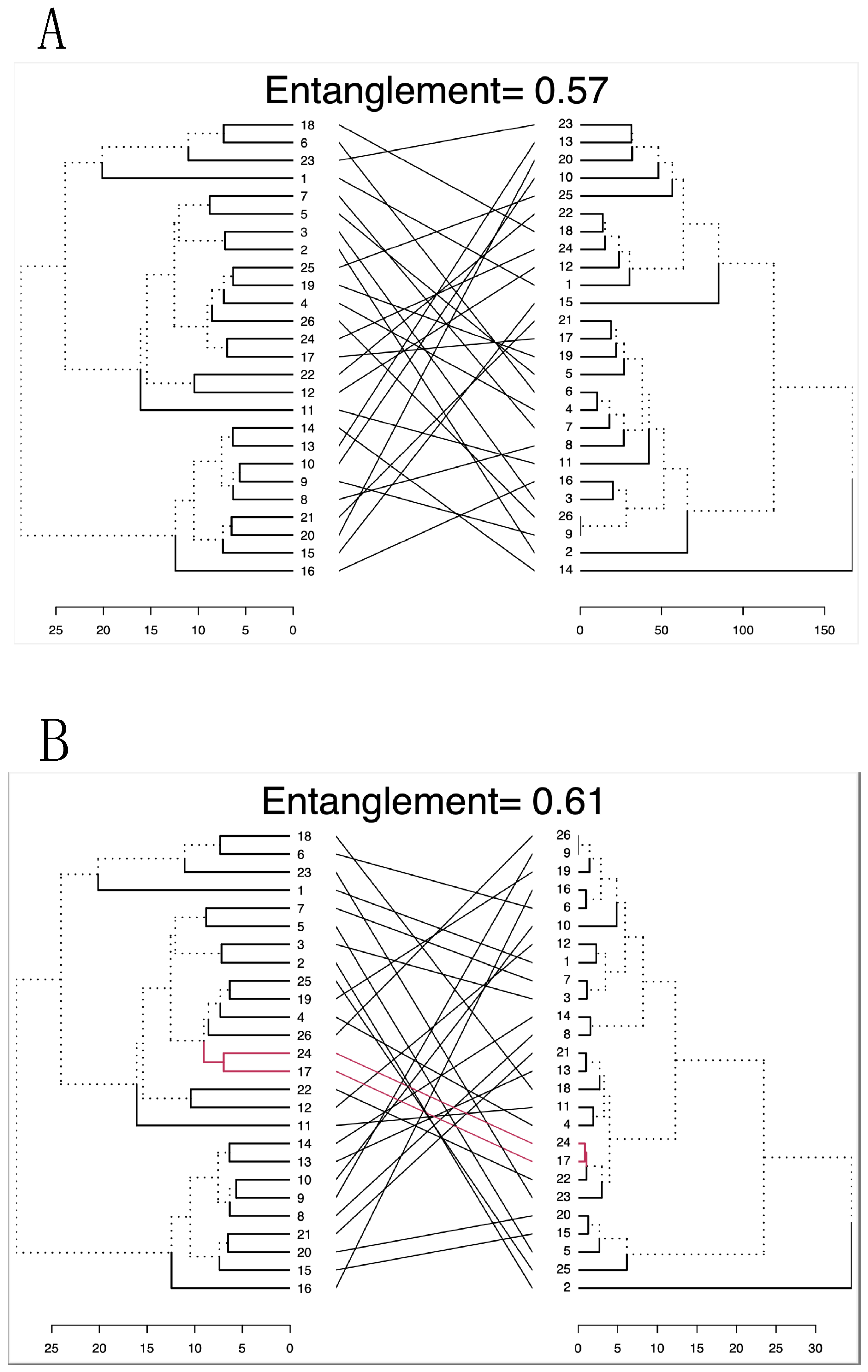
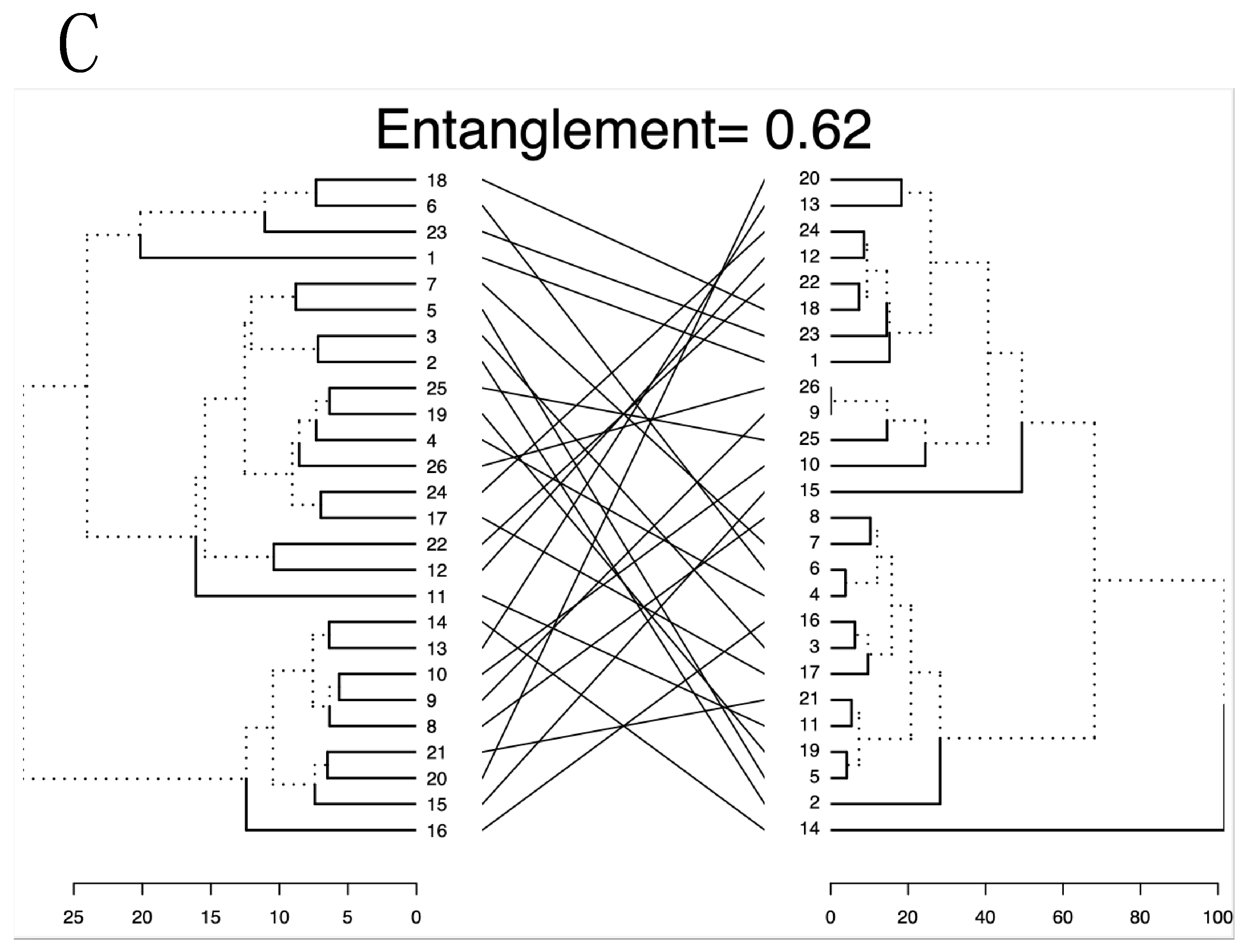
Figure 8 presents and visualizes the shape of the entanglement between the physical environmental parameters and sonic signatures. The red lines indicate an identical position in secondary branches of RSs. For instance, dendrogram branch # 17(RS41) and #24 (RS53) occupy the same position in both the environmental and sonic dendrograms.
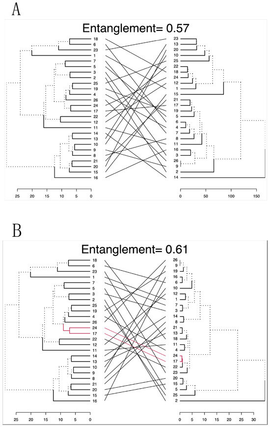

Figure 8.
Comparison between the dendrograms of the environmental parameters (left side) and the sonic signatures of each RS (A). In (B), the comparison is made using the sonic signatures derived from frequencies <2000 Hz, and in (C), using sonic signatures obtained from frequencies ≥2000 Hz. The alignment level is represented by the entanglement value, which ranges from 0 (complete misalignment) to 1 (perfect alignment). The numbers in the dendrogram indicate the order in which the RSs were included in the entanglement analysis. The correspondence between RS labels and their respective numbers is provided in Table S2. Dotted branches indicate that a branch in one dendrogram doesn’t have a good counterpart in the other.
Sonic indices were positively correlated with the woodland, shrubland, and bamboo landcover types. Conversely, sonic indices were negatively correlated for uncultivated and cultivated land types, olive orchards and vineyards, roads and buildings, and edgerows and altitude. Other landcover types, slope, and aspect/orientation were not significantly correlated with sonic indices (Table 4). The negatively correlated landcover classes of olive orchards, cultivated lands, and roads displayed a greater number of sonic index relationships compared to others. Bamboo was among the only positively correlated landcover class that had the highest number of relationships with sonic indices (Table 5). Olive orchards (27), Roads (14), and cultivated (13) have the highest number of significant sonic index correlations (Table 5).
Table 4.
Pearson correlation between sonic indices and landscape indicators (PN: Patch number, PA: Patch Area, PS: Patch Size, PP: Patch Perimeter, Fmax: maximum Feret Patch Dimension, Fmin: minimum Feret Patch Dimension, PFD: Patch Fractal Dimension). Negative significant correlations in bold and underlined.
Table 5.
Number of significant correlations between sonic indices and landcover types, represented by landscape indices, based on Table 4.
ENFBr and E were the sonic indices with the highest number of significant correlations with landcover classes (Table 5). Fmax, PN, PA, and Fmin were among the landscape indices that exhibited the highest number of correlations with the sonic indices.
4. Discussion
We investigated the complex relationships between the physical characteristics of a human-altered landscape and the sonic attributes of a Mediterranean small town. We found the spatial arrangement of the sonoscape is closely linked to the spatial configuration and distribution of landscape features. Understandably, this evidence indicates how physical features and land use practices profoundly impact ecological processes that generate and depend on the sonic environment. Particularly, this effect highlights the required needs and pressures soniferous species must adapt to in a changing environment [54].
Many montane regions of the Mediterranean basin are shaped by two interrelated processes: (1) urban development that is not only confined to large cities but also diffused into smaller ones, and (2) the depopulation of surrounding rural landscapes. The former has led to increased impervious surfaces and the destruction of soils, natural vegetation, and fauna. The latter has resulted in the concurrent loss or numerical reduction of several human companion species [55]. Both processes are harmful to the environment, particularly to biodiversity. Although abandonment theoretically allows nature to reclaim the area over the long term, in the short term, the ecological succession that follows promotes the spread of invasive, ubiquitous, cosmopolitan, and opportunistic species that do not contribute to creating or maintaining indigenous biodiversity and viable ecosystems resilient to change. This second condition is very common and more harmful than expected, with a particular impact on farmland birds [56,57]. Furthermore, the complete lack of data, at least regarding the sonic component, hinders any investigation requiring necessary comparisons, limiting a more holistic understanding of ecological responses to these human practices. Because the sonoscape serves as both an indicator of and influence on important ecological processes and species behaviors, without incorporating its significance into science and management practices simply perpetuates decision-making based on incomplete knowledge.
This void in ecological knowledge is what inspired us here to build upon two foundational studies conducted in the same region by Farina et al. [58] in the Magliano agricultural landscape and in a restored beech mountain forest by Farina and Mullet [22], both emphasizing the impact of land use transformations on avian fauna in southern Europe [59]. Our initial objective was to acquire the first documentation of a sonoscape’s spatial arrangement adhering to the sonotope model [58] when applied to an urban–rural landscape in the Tyrrhenian coastal area of northern Tuscany. Because previous studies in the United States [60,61], Australia [62], and India [63] have found spatial relationships between the sonoscape and landscape, we built upon this evidence to test our hypothesis that these spatial relationships also manifest within our study area. We applied sonic heterogeneity index SHItf and its sonic signature derivatives as another set of robust ecoacoustic indices to further describe and validate these sonic–environmental relationships.
We found an overall emerging pattern of sonic activities (i.e., sonic signature) that played out over the temporal period of spring–summer (April–June 2024). This was likely attributed to the fact that biophonies and technophonies in our study area are derived from the migratory and breeding behavior of birds and rise in human tourist activities during this time of year. Through our inferential cluster analysis of SHItf, we found that the ambient sounds captured by our spatially distributed grid of recorders exhibited specific groupings of similarly soniferous activities across the study area. These findings provide further evidence supporting the sonotope theory [22,58] that the sonoscape, like the landscape, is composed as a mosaic of homogeneous sonic patches (i.e., sonotopes).
Similarly, we found that our landscape indicators and landcover types were grouped into at least four distinct clusters that closely reflected the structural and geomorpholigical reality of the perceived landscape. More interestingly, the distinctive heterogeneity of landscape patterns in our study area presented the possibility that these sonotopes were attributed to specific landcover types and characteristics. In fact, sonic indices showed a number of significant correlations with landscape indicators and landcover types. Among the sonic indices, ENFBr and E exhibited the highest number of significant correlations with landcover classes. Sonic indices generally showed positive correlations with woodland, shrubland, and bamboo landcover types. In contrast, they were negatively correlated with uncultivated and cultivated lands, olive orchards, vineyards, roads, buildings, edgerows, and altitude. Notably, negatively correlated landcover classes—such as olive orchards, cultivated lands, and roads—demonstrated a greater number of relationships with sonic indices compared to other classes. Among the positively correlated landcover types, bamboo exhibited the highest number of significant relationships with sonic indices.
When the frequency spectra were partitioned by low- (SHItf < 2000 Hz) and mid-high-frequency categories (SHItf ≥ 2000 Hz) as representatives of geophony–technophony and biophony, respectively, we found that frequencies associated with geophony and technophony displayed better aggregations as sonotopes compared to frequencies attributed to biophony. Therefore, it is reasonable to assume that geophony and technophony possess a stronger relationship to the physical landscape than do biophonies. We suspect that this observation is primarily due to the sources of geophonies and technophonies, which are often fixed in space. In this case, streams and roads are spatially fixed sources of geophony derived from the behavioral dynamics of water and technophony from vehicle sounds confined to impervious surfaces. The predominance of these sonic elements in landcover is simply as profuse as the extent of their source. Their ecological and spatial link to landcover in this case is elementary. This may also explain the inverse correlation between sonic indices and human-altered landcover types like cultivated land, roads, and olive orchards that are often near sources of geophony and technophony.
In contrast, when considering frequencies associated with biophony (SHItf ≥ 2000 Hz), sonotopes were more fragmented and widely distributed across space. In this case, because the sound sources are likely derived from birds, their volant behavior and ability to move across fragmented habitats freely conflates our ability to accurately predict a direct link between a specific landcover type and biophony. Mullet et al. [60] found that biophonies were predominantly linked to landscape features attributed to forest edges along rivers and wetlands. Yet, there is evidence indicating that biophony is significantly lower at edges where technophony is predominant (i.e., roads) than along forest edges that border more natural landcover features where technophonies are absent [64,65,66,67]. The sonic effect from road traffic is pervasive enough that the low-frequency technophony it generates has been known to penetrate forest communities up to 300–350 m from the road source [65,67]. Road technophony appears to have a negative effect on biophonic activity [60,65,67], and the extent of roads within our study area certainly affects the spatial distribution of biophony.
Because these sonic–environmental links present both strong and weak correlations, clear interpretation and predictions of their ecological behavior beyond this study are challenging. While this is not uncommon to many ecological investigations, we acknowledge that it is not possible to generalize the effectiveness of these ecoacoustic indices, irrespective of landcover type and the metrics used for its characteristics [68]. However, each ecoacoustic index is more or less effective, depending on the landcover considered. This highlights how the intrinsic structure of landcover influences sonic expressions and the capacity of ecoacoustic indices to be predictive. Therefore, the intersection between landscape indices and ecoacoustic indices shows that the landcover type is a key factor in verifying the correlations between these metrics. This opens a new interpretative scenario for ecoacoustic approaches, where, at least in heterogeneous environments such as the one under investigation, it is not possible to assign predictive value to ecoacoustic indices irrespective of landcover type.
In ecoacoustics, the adoption of sonic indices is still a subject of debate, and recommendations are primarily based on a limited amount of empirical evidence [62,69]. Here, we adopted the SHItf index and some derivative metrics, for which we have information regarding their mathematical robustness and ecological significance [33], while avoiding the use of indices that are either mathematically untested or insufficiently interpreted ecologically. The different landcover categories exhibited varying sensitivities to sonic indices, depending on the landscape indicator used, as clearly highlighted in Table 4 and the two summary tables (Table 5 and Table 6).
Table 6.
Number of significant correlations of landscape indices for each landcover category, based on Table 4.
We consider this result particularly interesting because it demonstrates that the internal structure of each landcover type requires an appropriate descriptor to establish a relationship with sonic indices. The same holds true for the sonic indices themselves. These indices are a direct derivation of the SHItf and confirm the validity of this index, which is among the most widely used in ecoacoustics [70]. Notably, it is clear that the most effective sonic indices, such as ENFBr and E (Sheldon’s Evenness), are those that describe how frequencies are distributed within the sonic signature. Both indices were used for the first time in ecoacoustics and merit significant attention due to the excellent results they produced.
Ultimately, this study demonstrates that as the landcover category varies, it is necessary to employ a broad spectrum of landscape indices (seven in our case), which should be cross-referenced with an equally broad range of SHItf, sonic indices to reasonably establish the relationship between landscape and sonoscape.
5. Conclusions
As expected, the absence of generalizable patterns is the most notable result of this study. The sonotopes identified in the analysis form small clusters, primarily due to the landscape’s heterogeneity. While landscape indicators, when considered collectively, do not align with the sonic characteristics of the recording stations (RSs), individual sonic indices show significant correlations with certain landscape indicators specific to particular landcovers. This suggests that the landscape’s heterogeneity inhibits a direct collective correspondence with sonic sources, and that local conditions tend to favor one factor over another. The environmental uniqueness of the RSs influences both the sound sources, which alternate between technophony and biophony, and the modes of sound transmission, which can affect different volumes of the surrounding area. This analysis further confirms the validity of SHItf when expressed through its indices, demonstrating its effectiveness as a descriptor of ecological processes. The next step will involve a detailed analysis of biophonic manifestations. The methods we employed to extract data characterizing this landscape, the approaches for analyzing sound data, and the inferential analysis between these two domains have yielded valuable foundational results that are applicable in practical contexts and pave the way for future monitoring plans.
Supplementary Materials
The following supporting information can be downloaded at: https://www.mdpi.com/article/10.3390/acoustics7020023/s1, Figure S1; Figure S2; Figure S3. Table S1: Summary description of the eleven land cover categories.; Table S2: Maximum, minimum, and mean elevation above sea level (a.s.l.) for each Recording Station (RS). The slope is expressed in degrees. The variability in slope orientation ranges from 4 to 2. The "#" represents the order in which the RS were included in the entanglement analysis, as shown in Figure 8; Table S3; Table S4: Summary of the registration days aggregated by month and by recording station (RS), producing an overall total or recorded days.
Author Contributions
Conceptualization, A.F. and T.C.M.; methodology, A.F.; formal analysis, A.F.; investigation, A.F.; data curation, A.F. and T.C.M.; writing—original draft preparation, A.F. and T.C.M.; writing—review and editing, A.F. and T.C.M. All authors have read and agreed to the published version of the manuscript.
Funding
This research received no external funding.
Data Availability Statement
The original contributions presented in this study are included in the article/Supplementary Material. Further inquiries can be directed to the corresponding author.
Acknowledgments
We would like to express our gratitude to Enrico Tognari of Lunilettronik for generously donating 30 SETs and to the Mayor of the Municipality of Fivizzano, Pierluigi Giannetti, for granting us permission to install the recording equipment on public land.
Conflicts of Interest
The authors declare no conflicts of interest.
References
- Cardinale, B.J.; Duffy, J.E.; Gonzalez, A.; Hooper, D.U.; Perrings, C.; Venail, P.; Naeem, S. Biodiversity loss and its impact on humanity. Nature 2012, 486, 59–67. [Google Scholar] [CrossRef] [PubMed]
- Tilman, D.; Isbell, F.; Cowles, J.M. Biodiversity and ecosystem functioning. Annu. Rev. Ecol. Evol. Syst. 2014, 45, 471–493. [Google Scholar] [CrossRef]
- Pinilla, V.; Ayuda, M.I.; Saez, L.A. Rural Depopulation in Mediterranean Western Europe: A Case Study of Aragon. 2006, Documentos de Trabajo, 1. Available online: https://www.researchgate.net/publication/28143754_Rural_depopulation_in_mediterranean_western_Europe_a_case_Study_of_Aragon (accessed on 4 October 2024).
- Viñas, C.D. Depopulation processes in European rural areas: A case study of Cantabria (Spain). Eur. Countrys. 2019, 11, 341–369. [Google Scholar] [CrossRef]
- Sueur, J.; Farina, A. Ecoacoustics: The ecological investigation and interpretation of environmental sound. Biosemiotics 2015, 8, 493–502. [Google Scholar] [CrossRef]
- Farina, A.; Krause, B.; Mullet, T.C. An exploration of ecoacoustics and its applications in conservation ecology. Biosystems 2024, 245, 105296. [Google Scholar] [CrossRef]
- Stowell, D.; Sueur, J. Ecoacoustics: Acoustic sensing for biodiversity monitoring at scale. Remote Sens. Ecol. Conserv. 2020, 6, 217–219. [Google Scholar] [CrossRef]
- Lawrence, B.T.; Hornberg, J.; Schröer, K.; Djeudeu, D.; Haselhoff, T.; Ahmed, S.; Moebus, S.; Gruehn, D. Linking ecoacoustic indices to psychoacoustic perception of the urban acoustic environment. Ecol. Indic. 2023, 155, 111023. [Google Scholar] [CrossRef]
- Mullet, T.C.; Morton, J.M.; Gage, S.H.; Huettmann, F. Acoustic footprint of snowmobile noise and natural quiet refugia in an Alaskan wilderness. Nat. Areas J. 2017, 37, 332–349. [Google Scholar] [CrossRef]
- Krause, B.; Farina, A. Using ecoacoustic methods to survey the impacts of climate change on biodiversity. Biol. Conserv. 2016, 195, 245–254. [Google Scholar] [CrossRef]
- Mullet, T.C.; Farina, A.; Morton, J.M.; Wilhelm, S.R. Seasonal sonic patterns reveal phenological phases (sonophases) associated with climate change in subarctic Alaska. Front. Ecol. Evol. 2024, 12, 1345558. [Google Scholar] [CrossRef]
- Linke, S.; Gifford, T.; Desjonquères, C.; Tonolla, D.; Aubin, T.; Barclay, L.; Karaconstantis, C.; Kennard, M.J.; Rybak, F.; Sueur, J. Freshwater ecoacoustics as a tool for continuous ecosystem monitoring. Front. Ecol. Environ. 2018, 16, 231–238. [Google Scholar] [CrossRef]
- Stansfeld, S.A.; Matheson, P.M. Noise pollution: Non-auditory effects on health. Br. Med. Bull. 2003, 68, 243–257. [Google Scholar] [CrossRef]
- Alvarsson, J.J.; Wiens, S.; Nilsson, M.E. Stress recovery during exposure to nature sound and environmental noise. Int. J. Environ. Res. Public Health 2010, 7, 1036–1046. [Google Scholar] [CrossRef]
- Robinson, J.M.; Annells, A.; Cavagnaro, T.R.; Liddicoat, C.; Rogers, H.; Taylor, A.; Breed, M.F. Monitoring soil fauna with ecoacoustics. Proc. R. Soc. B 2024, 291, 20241595. [Google Scholar] [CrossRef] [PubMed]
- Quinn, C.A.; Burns, P.; Gill, G.; Baligar, S.; Snyder, R.L.; Salas, L.; Goetz, S.J.; Clark, M.L. Soundscape classification with convolutional neural networks reveals temporal and geographic patterns in ecoacoustic data. Ecol. Indic. 2022, 138, 108831. [Google Scholar] [CrossRef]
- IPCC. Climate Change 2021: The Physical Science Basis, in Contribution of Working Group I to the Sixth Assessment Report of the Intergovernmental Panel. 2021. Available online: https://www.ipcc.ch/report/ar6/wg1/ (accessed on 4 October 2024).
- Oleson, K.W.; Monaghan, A.; Wilhelmi, O.; Barlage, M.; Brunsell, N.; Feddema, J.; Hu, L.; Steinhoff, D.F. Interactions between urbanization, heat stress, and climate change. Clim. Change 2015, 129, 525–541. [Google Scholar] [CrossRef]
- Ameen RF, M.; Mourshed, M.; Li, H. A critical review of environmental assessment tools for sustainable urban design. Environmental Impact. Assess. Rev. 2015, 55, 110–125. [Google Scholar]
- Pauleit, S.; Duhme, F. Assessing the environmental performance of land cover types for urban planning. Landsc. Urban Plan. 2000, 52, 1–20. [Google Scholar] [CrossRef]
- Rapetti, F.; Vittorini, S. Note illustrative della carta climatica della Toscana. Atti Soc. Tosc. Sci. Nat. Mem. Ser A 2012, 117, 41–74. [Google Scholar]
- Farina, A.; Mullet, T.C. Sonotope patterns within a mountain beech forest of Northern Italy: A methodological and empirical approach. Front. Ecol. Evol. 2024, 12, 1341760. [Google Scholar] [CrossRef]
- Yip, D.; Leston, L.; Bayne, E.; Sólymos, P.; Grover, A. Experimentally derived detection distances from audio recordings and human observers enable integrated analysis of point count data. Avian Conserv. Ecol. 2017, 12, 11. [Google Scholar] [CrossRef]
- Schindelin, J.; Arganda-Carreras, I.; Frise, E.; Kaynig, V.; Longair, M.; Pietzsch, T.; Preibisch, S.; Rueden, C.; Saalfeld, S.; Schmid, B.; et al. Fiji: An open-source platform for biological-image analysis. Nat. Methods 2012, 9, 676–682. [Google Scholar] [CrossRef]
- Niemelä, J.; Kotze, D.J. Fauna and habitat fragmentation: The use of Feret’s diameter in habitat connectivity studies. Conserv. Biol. 2005, 19, 1303–1311. [Google Scholar]
- Sullivan, D.E.; Dunning, J.B. Using morphometrics, including Feret’s diameter, to assess habitat fragmentation and species dispersal. Landsc. Ecol. 2011, 26, 89–100. [Google Scholar]
- Pimentel, D.; Zuniga, R. Invasive species and their impact on biodiversity and ecosystems: Using Feret’s diameter to track spread. Biol. Invasions 2007, 9, 413–424. [Google Scholar]
- Thompson, K.; McCarthy, L.A. Invasive plant morphology: Can Feret’s diameter predict spread patterns? Plant Ecol. 2010, 184, 249–259. [Google Scholar]
- Feder, J. The fractal dimension. In Fractals; Springer: Boston, MA, USA, 1988; pp. 6–30. [Google Scholar]
- Turner, L.A. Fractal geometry and its application to landscape ecology. J. Environ. Manag. 1990, 31, 353–363. [Google Scholar]
- Stoll, A.R.G.A. Quantifying landscape patterns using fractal geometry. Landscape Ecol. 2001, 16, 137–147. [Google Scholar]
- Campos, L.M.d.; Pessôa, G.T.P. Fractals in Ecology and Environmental Science. Ecol. Complex. 2005, 2, 1–16. [Google Scholar]
- Farina, A. The acoustic complexity index (ACI): Theoretical foundations, applied perspectives and semantics. OIKOS 2024, e10760. [Google Scholar] [CrossRef]
- Farina, A.; Li, P. Methods in Ecoacoustics. The Acoustic Complexity Index; Springer Nature: Cham, Switzerland, 2022. [Google Scholar]
- Lance, G.N.; Williams, W.T. Computer programs for hierarchical polythetic classification (“similarity analyses”). Comput. J. 1966, 9, 60–64. [Google Scholar] [CrossRef]
- Lance, G.N.; Williams, W.T. Computer Program for Classification. In Proceedings of the ANCCAC Conference, Canberra, Australia, 16–20 May 1966. Paper 12/3. [Google Scholar]
- Blondel, P.; Dell, B.; Suriyaprakasam, C. Acoustic signatures of shipping, weather and marine life: Comparison of NE Pacific and Arctic Soundscapes. In Proceedings of the Meetings on Acoustics 2020, Virtual, 9 September 2020; AIP Publishing: Melville, NY, USA, 2020; Volume 40. [Google Scholar]
- Gini, C. Variabilità e Mutabilità: Contributo allo Studio delle Distribuzioni e delle Relazioni Statistiche; Tipografia P. Cuppini: Bologna, Italy, 1912; 159p. [Google Scholar]
- Simpson, E.H. Measurement of diversity. Nature 1949, 163, 688. [Google Scholar] [CrossRef]
- Hill, M.O. Diversity and evenness: A unifying notation and its consequences. Ecology 1973, 54, 427–432. [Google Scholar] [CrossRef]
- Pielou, E.C. The measurement of diversity in different types of biological collections. J. Theor. Biol. 1966, 13, 131–144. [Google Scholar] [CrossRef]
- Shannon, C.E.; Weaver, W. The Mathematical Theory of Communication; University of Illinois Press: Urbana, IL, USA, 1963; 117p. [Google Scholar]
- Heip, C. A new index measuring evenness. J. Mar. Biol. Assoc. U.K. 1974, 54, 555–557. [Google Scholar] [CrossRef]
- Sheldon, A.L. Equitability indices: Dependence on the species count. Ecology 1969, 50, 466–467. [Google Scholar] [CrossRef]
- Hurlbert, S.H. The nonconcept of species diversity: A critique and alternative parameters. Ecology 1971, 52, 577–586. [Google Scholar] [CrossRef]
- Ricotta, C. On parametric evenness measures. J. Theor. Biol. 2003, 222, 189–197. [Google Scholar] [CrossRef]
- Kasten, E.P.; Gage, S.H.; Fox, J.; Joo, W. The remote environmental assessment laboratory’s acoustic library: An archive for studying soundscape ecology. Ecol. Informat. 2012, 12, 50–67. [Google Scholar] [CrossRef]
- Gage, S.H.; Axel, A.C. Visualization of temporal change in soundscape power of a Michigan lake habitat over a 4-year period. Ecol. Inform. 2014, 21, 100–109. [Google Scholar] [CrossRef]
- Kassambara, A. Practical Guide to Cluster Analysis in R: Unsupervised Machine Learning (Vol. 1), 2017, (Sthda). Available online: http://www.sthda.com (accessed on 4 October 2024).
- R Core Team. R: A Language and Environment of Statistical Computing. R. Foundation for Statistical Computing: Vienna, Austria, 2023. Available online: https://www.R-project.org/ (accessed on 4 October 2024).
- Goodman, L.A.; Kruskal, W.H. Measures of association for cross classifications. J. Am. Stat. Assoc. 1954, 49, 732–764. [Google Scholar]
- Baker, F.B. Stability of two hierarchical grouping techniques case I: Sensitivity to data errors. J. Am. Stat. Assoc. 1974, 69, 440–445. [Google Scholar] [CrossRef]
- SAS Institute Inc. JMP (18 Pro) [Computer Software]. 2023. Available online: https://www.jmp.com (accessed on 4 October 2024).
- Mullet, T.C.; Farina, A.; Gage, S.H. The acoustic habitat hypothesis: An ecoacoustics perspective on species habitat selection. Biosemiotics 2017, 10, 319–336. [Google Scholar] [CrossRef]
- Zakkak, S.; Radovic, A.; Nikolov, S.C.; Shumka, S.; Kakalis, L.; Kati, V. Assessing the effect of agricultural land abandonment on bird communities in southern-eastern Europe. J. Environ. Manag. 2015, 164, 171–179. [Google Scholar] [CrossRef] [PubMed]
- Farina, A. Landscape structure and breeding bird distribution in a sub-Mediterranean agro-ecosystem. Landsc. Ecol. 1997, 12, 365–378. [Google Scholar] [CrossRef]
- Salaverri, L.; Guitián, J.; Munilla, I.; Sobral, M. Bird richness decreases with the abandonment of agriculture in a rural region of SW Europe. Reg. Environ. Change 2019, 19, 245–250. [Google Scholar] [CrossRef]
- Farina, A.; Mullet, T.C.; Bazarbayeva, T.A.; Tazhibayeva, T.; Polyakova, S.; Li, P. Sonotopes reveal dynamic spatio-temporal patterns in a rural landscape of Northern Italy. Front. Ecol. Evol. 2023, 11, 1205272. [Google Scholar] [CrossRef]
- Butler, S.J.; Boccaccio, L.; Gregory, R.D.; Vorisek, P.; Norris, K. Quantifying the impact of land-use change to European farmland bird populations. Agric. Ecosyst. Environ. 2010, 137, 348–357. [Google Scholar] [CrossRef]
- Mullet, T.C.; Gage, S.H.; Morton, J.M.; Huettmann, F. Temporal and spatial variation of a winter soundscape in south-central Alaska. Landsc. Ecol. 2016, 31, 1117–1137. [Google Scholar] [CrossRef]
- Quinn, C.A.; Burns, P.; Hakkenberg, C.R.; Salas, L.; Pasch, B.; Goetz, S.J.; Clark, M.L. Soundscape components inform acoustic index patterns and refine estimates of bird species richness. Front. Remote Sens. 2023, 4, 1156837. [Google Scholar] [CrossRef]
- Fuller, S.; Axel, A.C.; Tucker, D.; Gage, S.H. Connecting soundscape to landscape: Which acoustic index best describes landscape configuration? Ecol. Indic. 2015, 58, 207–215. [Google Scholar] [CrossRef]
- Thakre, C.; Laxmi, V.; Kalawapudi, K.; Motghare, V.M.; Vijay, R. Noise Mapping and Impact of Land Use Land Cover on Urban Soundscape. MAPAN 2025, 40, 59–75. [Google Scholar] [CrossRef]
- Morton, E.S. Ecological sources of selection on avian sounds. Am. Nat. 1975, 109, 17–34. [Google Scholar] [CrossRef]
- Pocock, Z.; Lawrence, R.E. How Far into a Forest does the Effect of a Road Extend? Defining Road Edge Effect in Eucalypt Forests of South-Eastern Australia. 2005. Available online: https://escholarship.org/uc/item/4q576877 (accessed on 4 October 2024).
- Terraube, J.; Archaux, F.; Deconchat, M.; Van Halder, I.; Jactel, H.; Barbaro, L. Forest edges have high conservation value for bird communities in mosaic landscapes. Ecol. Evol. 2016, 6, 5178–5189. [Google Scholar] [CrossRef]
- Munro, J.; Williamson, I.; Fuller, S. Traffic noise impacts on urban forest soundscapes in south-eastern Australia. Austral Ecol. 2018, 43, 180–190. [Google Scholar] [CrossRef]
- Shamon, H.; Paraskevopoulou, Z.; Kitzes, J.; Card, E.; Deichmann, L.J.; Boyce, J.A.; McShea, W.J. Using ecoacoustics metrices to track grassland bird richness across landscape gradients. Ecol. Indic. 2021, 120, 106928. [Google Scholar] [CrossRef]
- Bradfer-Lawrence, T.; Gardner, N.; Bunnefeld, L.; Bunnefeld, N.; Willis, G.S.; Dent, H.D. Guidelines for the use of acoustic indices in environmental research. Methods Ecol. Evol. 2019, 10, 1796–1807. [Google Scholar] [CrossRef]
- Xie, J.; Hu, K.; Zhu, M.; Guo, Y. Data-driven analysis of global research trends in bioacoustics and ecoacoustics from 1991 to 2008. Ecol. Inform. 2020, 57, 101068. [Google Scholar]


Disclaimer/Publisher’s Note: The statements, opinions and data contained in all publications are solely those of the individual author(s) and contributor(s) and not of MDPI and/or the editor(s). MDPI and/or the editor(s) disclaim responsibility for any injury to people or property resulting from any ideas, methods, instructions or products referred to in the content. |
© 2025 by the authors. Licensee MDPI, Basel, Switzerland. This article is an open access article distributed under the terms and conditions of the Creative Commons Attribution (CC BY) license (https://creativecommons.org/licenses/by/4.0/).