Article

Restoration for Intensity Nonuniformities with Discontinuities in Whole-Body MRI

by
Stathis Hadjidemetriou
1,*,
Ansgar Malich
2,3,
Lorenz Damian Rossknecht
2,3,
Luca Ferrarini
1 and
Ismini E. Papageorgiou
2,3
1
Department of Information Technologies, University of Limassol, 3–5 Chaidariou Street, Limassol 3020, Cyprus
2
Institute of Diagnostic and Interventional Radiology, Jena University Hospital, Friedrich Schiller University Jena, Am Klinikum 1, 07747 Jena, Germany
3
Institute of Radiology, Suedharz Hospital Nordhausen, Dr.-Robert-Koch-Str. 39, 99734 Nordhausen, Germany
*
Author to whom correspondence should be addressed.
Signals 2023, 4(4), 725-745; https://doi.org/10.3390/signals4040040
Submission received: 10 February 2023 / Revised: 25 August 2023 / Accepted: 9 October 2023 / Published: 18 October 2023

Abstract

:
The reconstruction in MRI assumes a uniform radio-frequency field. However, this is violated due to coil field nonuniformity and sensitivity variations. In whole-body MRI, the nonuniformities are more complex due to the imaging with multiple coils that typically have different overall sensitivities that result in sharp sensitivity changes at the junctions between adjacent coils. These lead to images with anatomically inconsequential intensity nonuniformities that include jump discontinuities of the intensity nonuniformities at the junctions corresponding to adjacent coils. The body is also imaged with multiple contrasts that result in images with different nonuniformities. A method is presented for the joint intensity uniformity restoration of two such images to achieve intensity homogenization. The effect of the spatial intensity distortion on the auto-co-occurrence statistics of each image as well as on the joint-co-occurrence statistics of the two images is modeled in terms of Point Spread Function (PSF). The PSFs and the non-stationary deconvolution of these PSFs from the statistics offer posterior Bayesian expectation estimates of the nonuniformity with Bayesian coring. Subsequently, a piecewise smoothness constraint is imposed for nonuniformity. This uses non-isotropic smoothing of the restoration field to allow the modeling of junction discontinuities. The implementation of the restoration method is iterative and imposes stability and validity constraints of the nonuniformity estimates. The effectiveness and accuracy of the method is demonstrated extensively with whole-body MRI image pairs of thirty-one cancer patients.

1. Introduction

Whole body (WB) MRI can be used to provide information about a variety of conditions. It has several applications for cancer imaging and patient monitoring. Some of these applications are metastases to the bones and other organs [1], refractory leukemia [2], and the ability to replace a PET/CT examination with a PET/MRI examination [3]. It is also used for general examination of asymptomatic individuals with predisposition to cancer [4]. Other applications are the imaging of extensive properties throughout the body such as fat distribution and for the imaging of metabolic disorders [5,6]. A more recent application is the treatment of inflammation that can also be extensive throughout the body [7]. The long-term objective for this type of imaging is to become a one-stop shop examination for the whole body as well as for the health status of as many individual organs as necessary.
However, WB-MRI imaging methodology and its uses are still under development. Hence, the acquired images suffer from several acquisition artifacts. These hamper not only the computerized analysis and quantification of the 3D data, but even the visual interpretation of the data by radiologists. One of the main imaging artifacts is the spatial intensity inhomogeneities throughout the human body. The imaging of the whole body can be performed with multiple coils. The images from individual coils suffer from smooth intensity nonuniformities that stem from the inhomogeneities of the radio-frequency (RF) field within the subject. The overall field also suffers from sharp changes in the inhomogeneities at the junctions between regions corresponding to adjacent coils. This is because the MRI signal amplitude across coils is not standardized and inevitably varies between the coils used due to multiple factors. There have been attempts to calibrate for smooth coil nonuniformities in MRI with physical phantoms and parametrized acquisitions [8,9]. In particular, in whole-body MRI, there is a method for station-to-station adapted B 1 + shimming [10]. However, these methods require additional physical acquisitions that are time-consuming and are valid for only particular MRI sequences and anatomies.
Several general postacquisition restoration methods have also been proposed. Postacquisition methods for intensity uniformity restoration benefit from regularity properties of the anatomy and of the physical radiofrequency (RF) field as well as from general prior knowledge of the imaging process. They are applicable to a range of MRI contrasts and anatomies. In general, they assume that the nonuniformity is smooth and that the underlying anatomic image is the union of piecewise constant intensity regions corresponding to different uniform tissues with uniform intensity transition magnitudes between them. Some postacquisition methods encode this directly using the total variation in space [11,12]. Piecewise anatomic constancy has also been encoded with local fuzzy C-means intensity clustering [13]. This method is also combined with level sets for spatial segmentation [14,15]. The entropy for the sharpness of the histogram has also been used [16]. A more general, non-parametric approach is the Bayesian coring framework. The image histogram has been analyzed with coring to remove noise [17,18]. Coring has been adapted for low-frequency noise to offer a smooth nonuniformity [19]. Current postacquisition methodologies in medical image analysis cannot accommodate sharp changes between intensity nonuniformities of different regions. Moreover, the direct histogram-based corrections can lead to an unstable dynamic range and hence unstable correction as well [19].
A clinical imaging protocol consists of multiple sequences providing images that suffer from different nonuniformities. Postacquisition methods have been developed for their joint restoration. A data dependent method fuses MRI with PET data [20]. A variational method preserves the differential structure of two images [21] and enforces a smooth nonuniformity. A statistical method minimizes the entropy of the joint histogram of two images [22]. Another method restores multiple co-registered images by minimizing the sum of the entropies of voxelwise stack vectors throughout an image [23].
In general, there has been significantly more work on homogenization of the intensities of an image rather than on standardization of the intensities of different parts of an image or standardization of intensities between several images. There have been efforts to account for the lack of intensity standardization in MRI by using physical arguments to compute physical MR imaging parameters of the tissues. These methods reconstruct intermediate homogeneous physical images [24,25]. Several postacquisition restoration methods have also been proposed. Histograms of pairs of images have been matched with piecewise linear transformations for brain images [26]. The difference between intensity ranges of different slices in a scan has been modeled with a multiplicative factor [27]. This multiplicative factor can vary for different slices. Histograms of images that can even be multicontrast have been normalized with the Kullbach–Leibler divergence [28]. A comparative study between different intensity standardization methods has found that more sophisticated methods that consider all images simultaneously either directly or at a pixel level improve performance [29]. Another study suggested that it is more appropriate to first perform intensity inhomogeneity correction and then to perform intensity standardization [30].
In WB-MRI, intensity standardization and intensity homogenization are intertwined. Thus, there has been some work on intensity standardization between different parts of an image and between different WB-MRI scans. A simple method identifies peak and trough features in the histograms of different coronal sections or stations. It then fits a continuum for these histogram features along the sections and stations [31]. However, different organs have different histograms, and organs can also contain pathologies that violate this continuity assumption. In a more comprehensive method, the joint intensity histogram of pairs of acquired images is non-rigidly registered to the joint histogram of reference images of the same contrasts to offer a vector field mapping the intensities to their corrected values [32,33]. Other methods are correcting based on overlapping regions of single-image blocks [34] or of their extension for multispectral image blocks [35]. This method is extended even further to start with a bias correction for the image of each coil separately using N4 [36,37]. It then continues to register the joint histograms of consecutive stations using their overlap as well as to register to a median station histogram to perform intensity standardization for the whole image [37].
Beyond smooth intensity nonuniformities, the method in this work needs to and does represent the abrupt changes in the intensity inhomogeneity field corresponding to the junctions between consecutive coils. The formation and preservation of discontinuities of the inhomogeneities under smoothing has been achieved with inhomogeneous diffusion also known as anisotropic diffusion. There has been a significant amount of work on these types of methods that preserve discontinuities across regions or equivalently smooth only within regions [38,39,40,41,42]. An early, but yet extensive, method for piecewise image smoothing and simultaneous noise estimation is based on the Minimum Description Length (MDL) principle formulation [41,42]. The method allows the separation of an image into piecewise smooth regions [41,42]. In effect, these methods are similar to the result of the solution of appropriate Euler–Lagrange partial differential equations [41,42]. Along the same lines, methods for solving geometric partial differential equations over the image domain have also been proposed [39,40]. Other early methods can separate the image only into piecewise constant components [38]. Image piecewise constancy has also been enforced with the L 1 norm constraint [43,44,45].
Some of the methods for anisotropic diffusion have been applied directly to biomedical MRI images for denoising [46,47]. Also, image piecewise smoothness has been combined with smoothness of the nonuniformity, e.g., retinex [11,12]. However, direct anisotropic diffusion of an image only assumes high-frequency spatial noise and incorrectly interprets shades and the discontinuities they can create as being due to image structure or anatomy [42,48]. Hence, in biomedical MRI, anisotropic diffusion methods interpret regions with different shading and abrupt transitions between them as the result of tissue differences. The proposed method addresses this limitation by applying the anisotropic diffusion to the shading nonuniformity artifact instead of applying it directly to the image. It thus obtains a piecewise smooth nonuniformity field.
The proposed postacquisition method performs a joint restoration of two images of the same anatomic region with different contrasts. The method uses a non-parametric Bayesian coring formulation for intensity restoration. This is applied to the statistical representation of the auto-co-occurrence statistics of each image as well as to the joint-co-occurrence statistics between the two images [49,50,51,52]. The effects of the intensity distortions on both types of co-occurrence statistics are modeled and restored. Their back-projection to the images offer rough initial estimates of the spatial nonuniformity corrections. The initial nonuniformity corrections are subsequently smoothed anisotropically to offer piecewise smooth nonuniformity corrections. Thus, the proposed restoration method can accommodate not only smooth intensity nonuniformities, but also sharp changes between the smooth intensity nonuniformities at the junctions between regions corresponding to consecutive coils. The MDL principle method that allows piecewise smoothness is used [41,42]. Additional constraints have also been imposed for the stability of the method. The proposed method has been tested and demonstrated extensively with anatomic WB-MRI datasets of 31 breast cancer patients.

2. Patient and Data Description

2.1. Study Design and Ethical Approval

The data are obtained from oncological clinical imaging of breast cancer or prostate cancer patients examined with WB-MRI imaging for possible bone metastases. The imaging data are for years between 2011 and 2019. The data were analyzed retrospectively, fully anonymized, in accordance with the ethical standards laid down in the 1964 Declaration of Helsinki and its amendments, the European Regulation 536/2014 and its latest addendum ICH GCP E6(R2)/2017, as well as with the guidelines of the Institutional Review Board (IRB) for clinical studies of the University of Jena (IRB number 2019-1452-Daten) (all datasets are anonymized and their sharing is enabled by the IRB licence. Sample datasets or all the datasets are available upon request (email) from the corresponding author).

2.2. Patients and Data Description

A total of 39 WB-MRI datasets were considered from an equal number of patients. The patient data were extracted from the database of the Suedharz Hospital Nordhausen for years 2011–2019 with a randomizer (https://www.randomizer.org/, last accessed on 9 February 2023). In the study, we randomly included 23 females (64.22 ± 7.61 y.o.), and 17 males (66.88 ± 6.74 y.o.); Student’s t-test, p = 0.51 ; normality was tested with the Kolmogorov–Smirnov test, p > 0.05 . No exclusion criteria were applied at this phase for the data.
The clinical images were acquired with a Philips Ingenia Suite 3.0 T or a 1.5 T static field strength using a dedicated dStreamWholeBody coil (Philips Healthcare Medical Systems, Hamburg, Germany) [53]. The protocol consists, among other sequences, of the two coronal sequences that in brief can be described as follows:
  • A T 1 -weighted ( T 1 w) sequence in a Turbo Spin Echo (TSE) or a Fast Field Echo (FFE) technique,
  • A Short Tau Inversion Recovery (STIR): This is an inverted pulse fat suppression method that, apart from the fat suppression, prolongs the T 1 w relaxation, and thus reduces the T 1 w signal. It furthermore prolongs the T 2 w relaxation, thus enhancing the T 2 w signal. All in all, STIR has an additive effect of enhancing the T 2 w signal. Thus, the STIR sequence offers T 1 weighted ( T 1 w) and T 2 weighted ( T 2 w) images, ( T 1 w + T 2 w) images.
The patient images from these two anatomic sequences are analyzed in this work. Some of the most important imaging protocol parameters in Table 1 are the same as those that have already been previously used [53]. As can be seen in Table 1, the 3D voxels in the datasets have anisotropic resolution. The resolution in the frontal (coronal) plane is higher than that along the front–back sagittal axis.
The complete WB-MRI images are an axial, y, concatenation of images from different coils placed along the patient. The body imaging data in this study were acquired with five such coils. Thus, the body image axial size is five times the axial size of the images described in Table 1. Since the images of the different coils are concatenated along the axial body direction, y, the junction planes between them are transverse on ( x , z ) . The intensity nonuniformities of individual coils are smooth. However, the nonuniformities at the junctions between different coils are sharp. The precise axial locations where images from different coils are joined are not preset and depend on the exact placement of the coils that can vary axially along the different patients.

2.3. Preparation of the Data

Both images, T 1 w TSE and T 1 w + T 2 w STIR, are denoised separately with median filtering. The denoised images are resampled to have identical spatial resolution that is chosen to be the lowest resolution of the two images. The resulting images may have different sizes. The largest image is cropped to that of the smallest along all axes so that the two images have the same size. In terms of intensity resolution, the acquired MRI images have four bytes per pixel. To save space and to increase processing speed, after limiting the dynamic range for the intensities, the number of bytes per pixel is reduced to two for both images. The common and simpler 3D grid and resolution for the two images simplifies significantly the subsequent image processing steps. The effect of the decrease in resolution of one of the two images is negligible without decreasing the accuracy of the nonuniformity estimation.

3. Methods

3.1. Spatial and Statistical Image Representation

3.1.1. Spatial Image Representation

The anatomic images of two different contrasts, I v i ( x ) , where x = ( x , y , z ) are spatial coordinates and i = 0 , 1 , have the same 3D sampling grid. They are assumed, respectively, to be the product of latent anatomic images I u i ( x ) with spatial intensity nonuniformities b i ( x ) due to MRI radio-frequency inhomogeneities and coils sensitivities. Each image is also corrupted with additive and independent noise, n i , to produce the image model as
I v i = b i · I u i + n i , i = 0 , 1 ,
where · is the voxelwise product. The first-order term of b i ( x ) provides a piecewise linear approximation within a spherical neighborhood N ρ of radius ρ . Median filtering applied to v i removes high-frequency noise n i .

3.1.2. Statistical Image Representation

The voxelwise probability distributions of I u ( x ) and b ( x ) , p u ( u ( x ) ) and p b ( b ( x ) ; 1 , σ b 2 ) , respectively, are assumed independent. The distortion of the joint intensity statistics is modeled by the non-stationary distribution p ( v | u ) ( v | u ) = p b v u | u = p b ( v u ; 0 , ( σ b u ) 2 ) . Thus, the intensity statistics of v, p v ( v ) , result from the convolution, ∗, p v ( v ) = p ( v | u ) ( v | u ) p u ( u ) = p u ( u ) p b v u ; 0 , ( σ b u ) 2 . The probability of the distortion is assumed to be bimodal with one mode for b ( x ) > 1 and another mode for b ( x ) < 1 and given by p b ( b ; 0 , σ b 2 ) = G b ; 0 , σ b 2 G 2 b ; 0 , σ b 2 + ϵ 2 , where ϵ 2 is a regularization constant.
The statistical representation of images v i are based on their intensities η i and their counts within neighborhood N ρ in image space to offer co-occurrence statistics as [49]
C v i v j ( v i , v j , η i , η j ) = C v i v j ( η i , η j ) = = x = I v i 1 ( η i ) x = I v j 1 ( η j ) x x 2 ρ d x d x ,
where ρ is the radius of the spherical neighborhood considered. The auto-co-occurrences result from i = j to produce C 00 and C 11 . The joint-co-occurrences are C 01 . The auto-co-occurrences are dominated by their diagonal, and thus the diagonal is weighted down with the sigmoid, 1 / ( 1 + e ( k 1 | η 0 η 1 | + k 2 ) ) , where k 1 and k 2 are constants. Examples of the co-occurrences of pairs of T 1 w and T 2 w images are presented in Figures 3 and 5.

3.2. Effect of Spatial Intensity Nonuniformities in Co-Occurrences

3.2.1. Distortion in Co-Occurrences from Spatial Intensity Nonuniformity

The statistics of the products b i . I u i are modeled as the convolutions of C u i u i and C u 0 u 1 with the respective PSF of the intensity distortions that are non-stationary to account for the spatial multiplication. The effects of b i in N ρ around x 0 are approximated by the zero-order term b ( x 0 ) that scales the auto-co-occurrences of C u i u i radially and the first-order term b ( x ) | x 0 that rotates them around the origin in the co-occurrence space [49]. The PSF affecting C u i u i is represented in polar coordinates ( r i , ϕ i ) . The σ r i of the PSF is scaled linearly with r i , σ r i r i . The σ ϕ of the PSF increases with ρ , is largest along the diagonal and is zero along the axes. The application of the PSFs of the distortions to p u i ( u i ) = C u i u i produce p v i ( v i ) = C v i v i with convolution
C v i v i ( r i , ϕ i ) = C u i u i ( r i , ϕ i ) p b ( r i ; 0 , σ r i 2 ) p b ( ϕ i ; 0 , σ ϕ i 2 ) , i = 0 , 1 ,
which represents the auto-co-occurrences of the distorted images.
The effects of the zero-order terms of b i on the joint-co-occurrences C u 0 u 1 of u i are in Cartesian coordinates. The σ η i of the PSFs are linearly related with η i , σ η i η i [50]. The diagonal relation between η i and r i is used, η i = r i / 2 . The application of the PSFs of the distortions to p u 0 u 1 ( u 0 , u 1 ) = C u 0 u 1 produces p v 0 v 1 ( v 0 , v 1 ) = C v 0 v 1 with convolution
C v 0 v 1 ( η 0 , η 1 ) = C u 0 u 1 ( η 0 , η 1 ) p b ( η 0 ; ( σ η 0 η 0 ) 2 ) p b ( η 1 ; ( σ η 1 η 1 ) 2 ) ,
which represents the joint-co-occurrences of the distorted images. The PSFs of the distortions are assumed separable.

3.2.2. Restoration from Spatial Non-Uniformity in Co-Occurrences

The Point Spread Function (PSF) for the distortion of the intensity co-occurrences increases linearly with intensity. Thus, the deconvolution is non-stationary. It appears that it is difficult to perform non-stationary deconvolution in the Fourier transform domain. Hence, in the proposed method, this deconvolution is performed directly in the spatial domain with the Van Cittert algorithm [54]. This is iterative with
p u n + 1 = p u n + β ( p v 0 p b p u n ) ,
where β is a regularization parameter, p v 0 are the statistics of the original image, and p b is the distortion PSF. The last iteration provides the estimate p ˜ u ( u ) .
The Van Cittert deconvolutions are non-stationary for both the radial and the angular dimensions of the auto-co-occurrences. The restorations of C v i v i provide C ˜ u i u i for i = 0 , 1 . The restoration of C v 0 v 1 provides C ˜ u 0 u 1 .

3.3. Bayesian Posterior Expectation for the Restoration

An overview of the posterior expectation is presented in Figure 1. The posterior expectation of the latent intensity, u ^ = E ( u | v ) , is the minimum mean squared error. The Bayesian expansion for p ( u | v ) ( u | v ) produces
u ^ = E ( u | v ) = 0 p ( u | v ) ( u | v ) u d u = 0 p ( v | u ) ( v | u ) p u ( u ) u d u 0 p ( v | u ) ( v | u ) p u ( u ) d u .
The likelihood p ( v | u ) ( v | u ) in Equation (6) is the non-stationary distortion as given in Section 3.1 for the joint intensity statistics. This expression expanded in Equation (6) also involves the prior distribution p u ( u ) of latent image u. This is estimated in Equation (5) with the deconvolution of the distortion p b ( v u | u ) from the intensity co-occurrence distribution p v ( v ) , ( C v ), to provide the non-parametric prior p ˜ u ( u ) = C ˜ u of u. These two factors are substituted into Equation (6) to produce
u ^ = E ( u | v ) = 0 p b ( v u ; 0 , ( σ b u ) 2 ) · p ˜ u ( u ) · u d u 0 p b ( v u ; 0 , ( σ b u ) 2 ) · p ˜ u ( u ) d u .
The magnitude of p b ( v u ; ( σ b u ) 2 ) is significant for neighborhood u N u in co-occurrence space and tends to zero for intensities u far from v. The image domain is discrete and the necessary discretization of u ^ = E ( u | v ) in Equation (7) becomes
u ^ = E ( u | v ) = u N u P b ( u ; 0 , ( σ b u ) 2 ) · C ˜ u ( u + u ) · ( u + u ) u N u P b ( u ; 0 , ( σ b u ) 2 ) · C ˜ u ( u + u ) .
The extent of P b and N u increases linearly with intensity u.
General Equation (8) for the auto-co-occurrence statistics offers the posterior expectation of the intensities in polar coordinates ( r i ^ , ϕ i ^ ) T = E ( ( r i , ϕ i ) T | ( r i , ϕ i ) T ) in auto-co-occurrence neighborhoods r i N r i and ϕ i N ϕ i as
r i ^ ϕ i ^ = N r i N ϕ i P b r i ϕ i ; ( σ b , r i r i ) 2 σ b , ϕ i 2 · C ˜ u i u i r i + r i ϕ i + ϕ i · r i + r i ϕ i + ϕ i N r i N ϕ i P b r i ϕ i ; ( σ b , r i r i ) 2 σ b , ϕ i 2 · C ˜ u i u i r i + r i ϕ i + ϕ i ,
where P b ( r i , ϕ i ) is as used in the RHS of Equation (3). Equation (8) for the joint-co-occurrence statistics provides the posterior expectation of the intensities in Cartesian coordinates ( η 0 ^ , η 1 ^ ) T = E ( ( η 0 , η 1 ) T | ( η 0 , η 1 ) T ) in joint-co-occurrence neighborhoods η 0 N η 0 and η 1 N η 1 with
η 0 ^ η 1 ^ = N η 0 N η 1 P b η 0 η 1 ; ( σ b , η 0 η 0 ) 2 ( σ b , η 1 η 1 ) 2 C ˜ u 0 u 1 η 0 + η 0 η 1 + η 1 η 0 + η 0 η 1 + η 1 N η 0 N η 1 P b η 0 η 1 ; ( σ b , η 0 η 0 ) 2 ( σ b , η 1 η 1 ) 2 C ˜ u 0 u 1 η 0 + η 0 η 1 + η 1 ,
where P b ( η 0 , η 1 ) is as used in the RHS of Equation (4).

3.4. Spatial Image Restoration

3.4.1. Back-Projection of Restoration to Space

A scalar gain factor is computed for each intensity co-occurrence. The initial restoration field, b 1 ^ , is given by the Bayesian estimate u ^ from Equation (8) with
b 1 ^ ( x ) = E u ( x ) v ( x ) v ( x ) = E u ( x ) | v ( x ) v ( x ) = u ^ v .
This provides a voxelwise restoration factor independent of x . Thus, it is precomputed and stored in a 2D matrix with axes of sizes equal to the dynamic ranges of the corresponding images. The gain in Equation (11) for C u i u i in Equation (9) becomes R i , t s ( r , ϕ ) = r i ^ r i , i = 0 , 1 . The gain for C u 0 u 1 in Equation (10) becomes R i , t b = η i ^ η i , i = 0 , 1 . They offer 2D restoration matrices of dimensions equal to the corresponding dynamic ranges.
The intensity co-occurrences index the restoration matrices to provide an initial incremental estimate of the restoration with
b 1 ^ i ( x ) = 1 2 E x N ρ R i s v i ( x ) , v i ( x + x ) + R i b v 0 ( x ) , v 1 ( x + x ) .
This offers an initial rough restoration field in an image space.

3.4.2. Anisotropic Smoothing of the Restoration Field

The nonuniformities of individual coils are smooth and, in this case of multiple coils, they are piecewise smooth due to the differences between the sensitivities of different coils. In particular, the junctions between the coils are on axial planes ( x , z ) of the 3D data. Hence, the nonuniformities on axial planes ( x , z ) are unaffected and remain smooth. This is imposed to the initial rough estimates b 1 ^ ( x ) with a smooth 2D anisotropic axial spatial Gaussian filter G ( x , z ; σ s , i 2 ) . This filtering does not affect the piecewise nonuniformities in the axial direction resulting from different coils. It produces the restoration fields at this phase as
W i , t ( x ) = b 1 ^ i , t ( x ) G ( x , z ; σ s , i 2 ) , i = 0 , 1 .
The application of the restoration fields to the images produces I v i ( x ) I v i ( x ) W i , t ( x ) .
The piecewise nonuniformity along the axial direction, y, is accounted for with spatially varying inhomogeneous smoothing. The method used is based on the 2D Minimum Description Length (MDL) principle method that has been developed for piecewise smoothness of image regions [41,42]. In the 2D rectangular image grid, the 8-connected neighborhood in used. The 2D method considers the anisotropy of the grid. The method for 2D piecewise smoothness is extended in his work for 3D piecewise smoothness. In 3D, the 26-connected neighborhood is used. The considerations for the anisotropy artifact of the 8-connected neighborhood in the 2D grid are extended to account for the spatial anisotropy of the 26-connected neighborhood of the 3D grid used in this work. It considers the resolution of the 3D grid of the image within the neighborhood of the anisotropic filter.
The 3D anisotropic smoothing with MDL is applied to W i , t ( x ) to offer the final restoration field W. The MDL principle can be formulated equivalently in terms of the Bayesian Maximum a Posteriori (MAP) estimate. This uses the Bayesian formulation:
P ( W i | W i ) = P ( W i | W i ) P ( W i ) P ( W i ) , i = 0 , 1 ,
where W i offers initial rough estimates of the restoration and W i are the final restoration fields. In fact, in this case, it is the minimum rather than the maximum of the Bayesian posterior that is of interest. The MAP strategy is to choose the W i that minimizes P ( W i | W i ) . That is, the objective is to obtain the MAP estimate that is given by
W ^ i , M A P = arg min W i P ( W i | W i ) = ( 1 ) arg min W i P ( W i | W i ) P ( W i ) P ( W i ) = ( 2 ) arg min W i P ( W i | W i ) P ( W i ) .
Equality ( 1 ) in Equation (15) holds from the Bayesian formulation in Equation (14). Equality ( 2 ) in Equation (15) holds from the assumption that the marginal likelihood P ( W i ) is constant.
The probability of the likelihood P ( W i | W i ) is a Gaussian distribution of the noise P ( W i | W i ) = x ( W i W i ) with a zero mean and variance σ W 2 in the spatial nonuniformity. In the piecewise constant case, the probability of prior for a piecewise constant field W i is a Gaussian normal distribution of the length of the boundary between the different regions. The length of the boundary is P ( W i ) = x x ( 1 δ ( W i ( x ) W i ( x ) ) ) , where x and x are neighboring spatial locations. Substituting the likelihood and the prior in Equation (15) provides the MAP estimate as
W ^ i , M A P = arg min W i exp x W i W i σ W 2 + x x ( 1 δ ( W i ( x ) W i ( x ) ) ) = ( 1 ) arg min W i x W i W i σ W 2 + x x ( 1 δ ( W i ( x ) W i ( x ) ) ) .
Equality ( 1 ) of Equation (16) holds since the logarithm is a monotonic function. The cost for the piecewise constant case in Equation (16) can be extended for a piecewise linear field and even for piecewise fields of higher orders [41,42]. In this work, the degree of smoothness is set to linear.
The implementation of the MDL principle method uses the continuation method to deal with the discrete δ ( ) functions with a continuous optimization. That is, the implementation is iterative with K iterations. The extent of smoothing increases with the number of iterations K. The result is to obtain the piecewise smooth restoration field W i ( x ) for the nonuniformity.

3.5. Iterative and Stable Estimation of Cumulative Intensity Restoration

The restoration is iterative t = 0 , , t m a x 1 , where t m a x is the maximum number of iterations. The restoration field is first computed at each iteration, t, with anisotropic axial Gaussian smoothing of standard deviation that decreases with iterations, t, and is given by
σ s = 2 σ s 0 1 t t m a x 1 ,
where σ s 0 is a parameter for the spatial planar Gaussian smoothing. This smoothing as described in Equation (13) provides W i , i n c r , t ( x ) . That is, the axial anisotropic Gaussian smoothing at the first iteration t = 0 is maximal and at the last iteration t m a x 1 it is zero, σ s | t = t m a x 1 = 0 . It is then anisotropically smoothed with the MDL principle method with K iterations to provide W i , i n c r , t ( x ) . That is, at the last iteration, the smoothing consists exclusively of MDL principle anisotropic smoothing.

3.5.1. Incremental Nonuniformity Correction Field

As described in Equation (12) for t > = 0 , the intensity co-occurrences index the restoration matrices to provide an initial incremental estimate of the restoration with
b 1 ^ i , i n c , t ( x ) = 1 2 E x N ρ R i , t s v i ( x ) , v i ( x + x ) + R i , t b v 0 ( x ) , v 1 ( x + x ) .
This rough incremental estimate is further processed to compute the incremental intensity homogeneity field. It is first smoothed with an anisotropic Gaussian of σ s , i n c r , G ( x , z ; 0 , σ s , i n c r 2 ) , to provide W i , i n c r , t ( x ) , where a low-value σ s , i n c r is used. It is then filtered with the MDL anisotropic smoothing method with limited iterations K i n c r for the incremental restoration. The anisotropic smoothing offers the final incremental restoration field, W i , i n c r , t ( x ) .

3.5.2. Iterative Estimation of Cumulative Intensity Restoration

At t = 0 , the restoration fields are initialized to W i , c u m , t = 0 ( x ) = 1 , x . The cumulative restoration at subsequent time steps, t, is the product of the cumulative restoration at the previous iteration W i , c u m , t 1 of iteration t 1 with the estimates W i , i n c r , t ( x ) of incremental restoration at iteration t > 0 to offer the cumulative estimate of the restoration,
W i , c u m , t = W i , c u m , t 1 × W i , i n c , t 1 .
The estimates W i , c u m , t ( x ) are smoothed with a spatial Gaussian filter G ( x , z ; σ s , c u m 2 ) to offer cumulative restorations
W i , c u m , t ( x ) = W i , c u m , t ( x ) G ( x , z ; σ s , c u m 2 ) , i = 0 , 1 ,
where σ s , c u m > σ s , i n c r . The estimates of the field inhomogeneous smoothing are then piecewise smoothed with the MDL principle method with K c u m > K i n c r to produce W i , c u m , t .
The W i , c u m , t are applied to I v i , t 1 to provide I v i , t = I u i , t 1 that are the updated estimates for the latent images.

3.5.3. End Condition for the Iterations

The method runs for a maximum of t m a x = 10 iterations. The optimal iteration, t o p t , is the one for which the negative of the entropy of the joint intensity co-occurrence statistics, C 01 ,
H 01 , t = l , m C 01 , t ( l , m ) log C 01 , t ( l , m ) ,
is maximized. That is, the optimal iteration providing the restored images corresponds to t o p t = max t H 01 , t .

3.6. Valid Domains in Image Space and Statistics

The MRI acquisition sequences produce he Regions of Interest ( R O I ) of the images, I R O I , i , with valid signal. They also provide a valid dynamic range with tissues contrasts. However, the dynamic ranges of the MRI images are not standardized.

3.6.1. Valid Signal Region of Images

Signal nonuniformities, of course, presuppose the presence of a signal and hence only exist over the signal regions of the images. Thus, the signal regions of the images, I R O I , i , are extracted and further processed to compute the spatial intensity nonuniformities. The signal regions are identical for both images. To identify the signal regions, the two images are added. Otsu’s thresholding [55] applied to their sum image offers the foreground, I F G , image. This preliminary foreground is morphologically closed with a structuring element, S . This produces the signal region, the foreground, that is, the Region of Interest (ROI), as I R O I = I F G S .

3.6.2. Valid Dynamic Co-Occurrence Ranges in Statistics

The nonuniformities are over the signals regions of the images and affect their dynamic ranges and contrasts. The upper parts of the images dynamic ranges may correspond to artifacts and are compressed linearly in the proposed method. To achieve this, reference intensities η i , r e f for high cumulative percentages, 90 % , of the dynamic ranges are computed. The dynamic ranges of the noise are delimited by the minimum signal intensities, η i , m i n = 0.1 × η i , r e f . The dynamic ranges are preserved up to η i , u p p = 1.5 × η i , r e f . Beyond these values the intensity ranges are compressed linearly up to η i , m a x = 3.0 × η i , r e f for ranges [ 1.5 × η i 0.9 , 3.0 × η i 0.9 ] . The dynamic ranges are scaled linearly so that η i , m a x become intensity 500, that is, η i , m a x 500 . This value is a tradeoff between intensity resolution and computational complexity for processing the statistics. After the intensity scaling, the direct computation of the statistics from the images would create spikes in the statistics in cases where a dynamic range is compressed and voids in cases where a dynamic range is expanded. To avoid these artifacts in the statistics, noise of a very small standard deviation, 0.5 , is added to both images.
The intensity ranges of [ η i m i n , η i m a x ] = [ 0.1 η i , r e f , 3 η i , r e f ] are assumed to correspond to the valid signal regions of the R O I s, I R O I , i = 1 . The regions in the images ROIs with intensities in ranges [ 0 , η i m i n ] and intensities beyond η i m a x are invalid, I R O I , i = 0 .
The C i i are computed over ( [ η i , m i n , η i , m a x ] 2 ) . The same ranges are used for the deconvolution of the C i i to give the R i s . The deconvolution of C i j for R i b considers [ η i , m i n , η i , m a x ] for i and the range starting from zero [ 0 , η j , m a x ] for image j. Beyond the valid ranges, the entries of R i are set to unity, R i s = R i b = 1 .
The estimates of the initial restoration fields b 1 ^ i , i n c in Equation (12) involve window N ρ in image space over the valid part of the ROI of image i and is set to the neutral value of unity outside. The resulting estimates are spatially smoothed with a Gaussian to give W i with a window depending on σ s in Equation (13). The smoothing windows of the nonuniformity with Equation (13) consider a spatial multiplicative field with unit weight in the corresponding valid region I R O I , i = 1 and with value much less than unity in the remaining ROI. As a result the spatial Gaussian smoothing gives smoothly unity farther from the valid region and towards the invalid region of the image with I R O I , i ( x ) = 0 .

3.6.3. Stability of Valid Co-Occurrence Ranges along the Iterations

The valid image domains in space remain the same along iterations and are the originally computed ROIs, I R O I , i . The stability of the dynamic ranges are also ensured. The first constraint to this end is applied to the output of Equation (12) to set the pixelwise average of the restoration to unity with normalization
b 1 ^ i , i n c , t ( x ) b 1 ^ i , i n c , t ( x ) b 1 ^ i , i n c , t ( x ) 1 .
A second constraint preserves the reference intensity so that η i , r e f , t = η i , r e f , t = 0 , by rescaling the restorations from Equation (13) with
W i , t W i , t × η i , r e f , t = 0 η i , r e f , t .
These two constraints in Equations (22) and (23) ensure stability of the dynamic ranges by avoiding both darkening and saturation of the dynamic ranges of the images.

4. Experimental Results

4.1. Data Quality

The imaging data and their statistics are first examined by eye for quality control. Some image pairs of patients have extensive misregistration artifacts. This misregistration is often due to motion of the shoulders and the legs of the patient. The misregistration is also due to differences in the fields of view between the two images of a patient, particularly in the front-to-back, or sagittal, axis. In the cases where the images of a patient suffer from this artifact and are misregistered, the images are excluded from further analysis.
The intensity statistics of the whole image is the sum of the statistics from the images of the various coils. In this study, the statistics are the intensity co-occurrences. In some cases, the intensity range corresponding to noise in one of the coil images overlaps with the intensity range of the signal in another one of the coil images. In these cases, the noise intensity range and hence noise image region cannot be discriminated from the signal intensity range in the statistics of the whole image. The image sets of a patient that suffer from such extreme acquisition artifact are excluded from the automated image analysis.
Overall, six images suffer from misregistration artifacts and two images suffer from the signal acquisition artifact. Thus, out of a total of 39 images, there are 31 valid images that are considered in this study.

4.2. Implementation

4.2.1. Parameters of the Method and Their Values

The size of the spherical window for the computation of the co-occurrences is ρ = 24 mm. Within a sphere of this size, the nonuniformity field is assumed constant or piecewise constant. To expedite computation, a subsampling step set to ρ s t e p = 4 mm is used. As described in Section 3.2.1, the standard deviation of the deconvolution filter for the co-occurrence statistics is σ r i r i , where r i is the magnitude of the co-occurrences. The standard deviation of the deconvolution filter for the joint-co-occurrence statistics is σ η i η i , where η i is the magnitude of the joint-co-occurrences. The maximum values of the standard deviations of the deconvolution filters, σ r i and σ η i , at the maxima of the dynamic ranges are set to 6 % of these dynamic ranges extents. The standard deviations of the deconvolution filers are accumulated along the iterations, t m a x = 10 , to cumulatively remove the total standard deviations of the distortions present in the statistics.
The Gaussian filtering for the rough nonuniformity estimates is implemented with separable Gaussian filtering along the two axes of the transverse plane of the image. There is no Gaussian smoothing in the axial direction y. The rough estimate of the nonuniformity after the preliminary smoothing with the Gaussian is processed with the MDL principle 3D anisotropic smoothing to separate the field into piecewise linear regions. Higher orders for the MDL smoothing are possible, and in some cases would be more representable. However, they would significantly increase the computational complexity of the MDL smoothing. The size of the windows for MDL smoothing is 3 × 3 × 3 with associated weights for each location inversely proportional to the distance of the voxels in space from the center considering anisotropy. The extent of the incremental smoothing both for the case of anisotropic Gaussian smoothing and anisotropic MDL smoothing is 33 % of the extent for the respective cumulative smoothing. That is, σ s , i n c r = 1 3 σ s , c u m and K i n c r = 1 3 K c u m . The cumulative smoothing parameter values are σ s , c u m =107 mm and K c u m = 15 . A lower smoothing for the incremental nonuniformity is used to avoid discontinuities in the incremental nonuniformity field that is also assumed to be smooth. A larger smoothing for the cumulative nonuniformity fields represents the actual coil field nonuniformities.
The size of the images is very large. To expedite processing, the images are subsampled by a certain factor along each of their axes. In the experiments, this factor is α = 0.5 . That is, the number of pixels in the subsampled image is only 12.5 % of the number of pixels in the original image. The values of several of the program parameters, namely ρ , ρ s t e p , σ s , c u m , decrease proportionately to the image axes subsampling factor, α . That is, the parameters become ρ Signals 04 00040 i001 α ρ , ρ s t e p Signals 04 00040 i001 α ρ s t e p , and σ s , c u m Signals 04 00040 i001 α σ s , c u m . The value of the parameter α is a tradeoff between computational complexity and accuracy of the method.

4.2.2. Computational Complexity of the Method

The size of the 3D image I is taken to be approximately I 200 × 150 × 60 2 × 10 6 . The size of the statistics using the dynamic ranges is η i m a x 2 = 500 × 500 = 0.25 × 10 6 . The order of the cost of the main steps of the method per iteration t is as follows:
  • Computation of the co-occurrence and the joint co-occurrence statistics:
    3 I ρ ρ 2 6 × 10 6 × ρ ρ 2 .
  • Deconvolution of the statistics: 3 η i m a x 2 σ η 2 = 0.75 × 10 6 × σ η 2 .
  • Back-projection to the image: 3 I ρ ρ 2 6 × 10 6 × ρ ρ 2 .
  • Gaussian smoothing of spatial nonuniformity: 2 I σ s , c u m 2 4 × 10 6 × σ s , c u m 2 .
  • MDL smoothing of spatial nonuniformity: 2 I 3 3 K c u m 108 × 10 6 × K c u m , where 3 3 is the connectedness in MDL smoothing.
  • Multiplication of incremental spatial nonuniformity with cumulative spatial nonuniformity: I 2 × 10 6 .
The size of the 3D image, I , is larger than the size of the 2D co-occurrence statistics, η i m a x 2 . Therefore, the image domain operations for the spatial nonuniformity dominate. The costs of computing the co-occurrence statistics and of back-projecting them to the image are almost the same. The most expensive image-based operation is the cost of MDL smoothing of the nonuniformity. Its cost is greater for larger values of the number of iterations K c u m compared to the number of the co-occurrence sampling pixels, ρ ρ 2 .

4.3. Experiments and Validation with Whole-Body Images

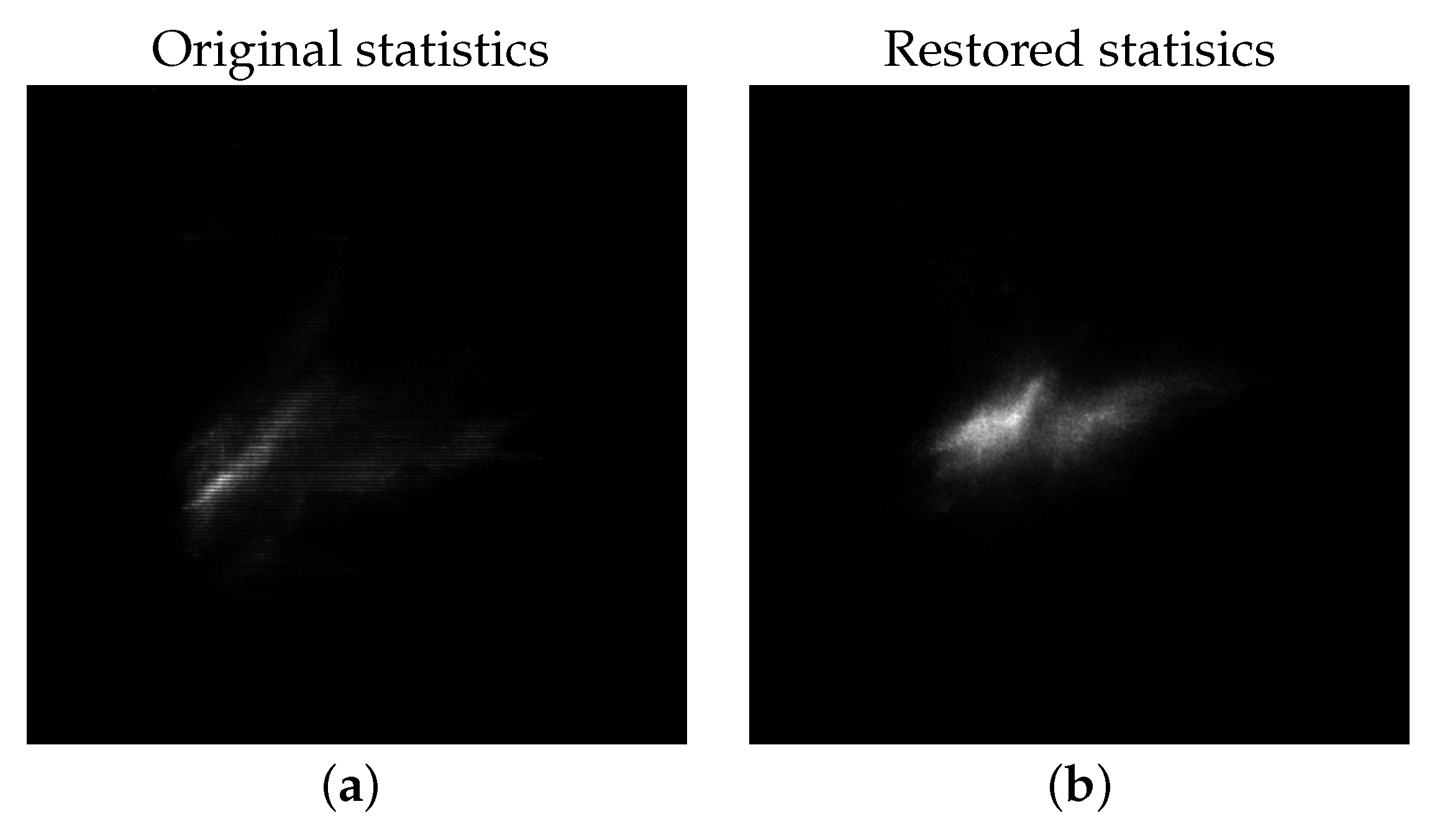
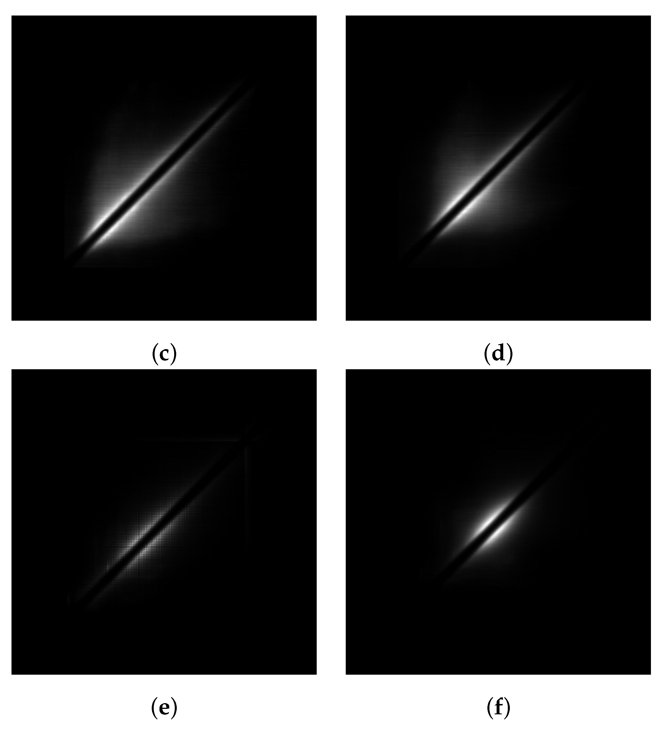
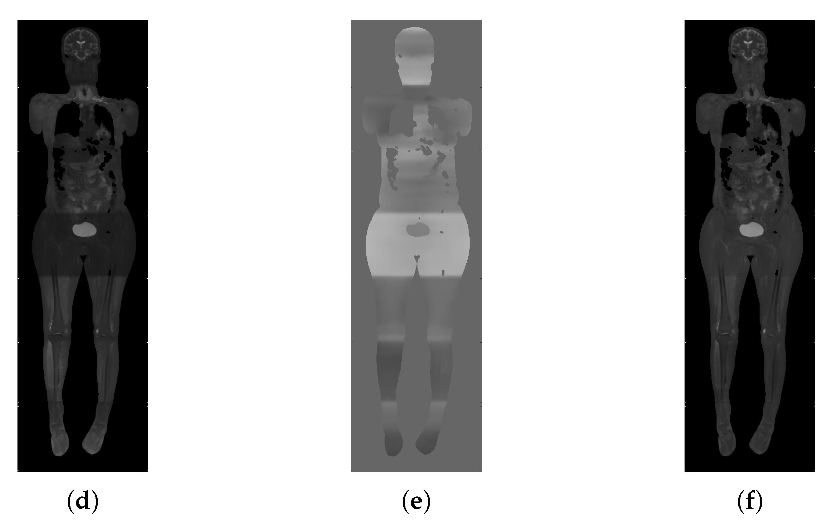
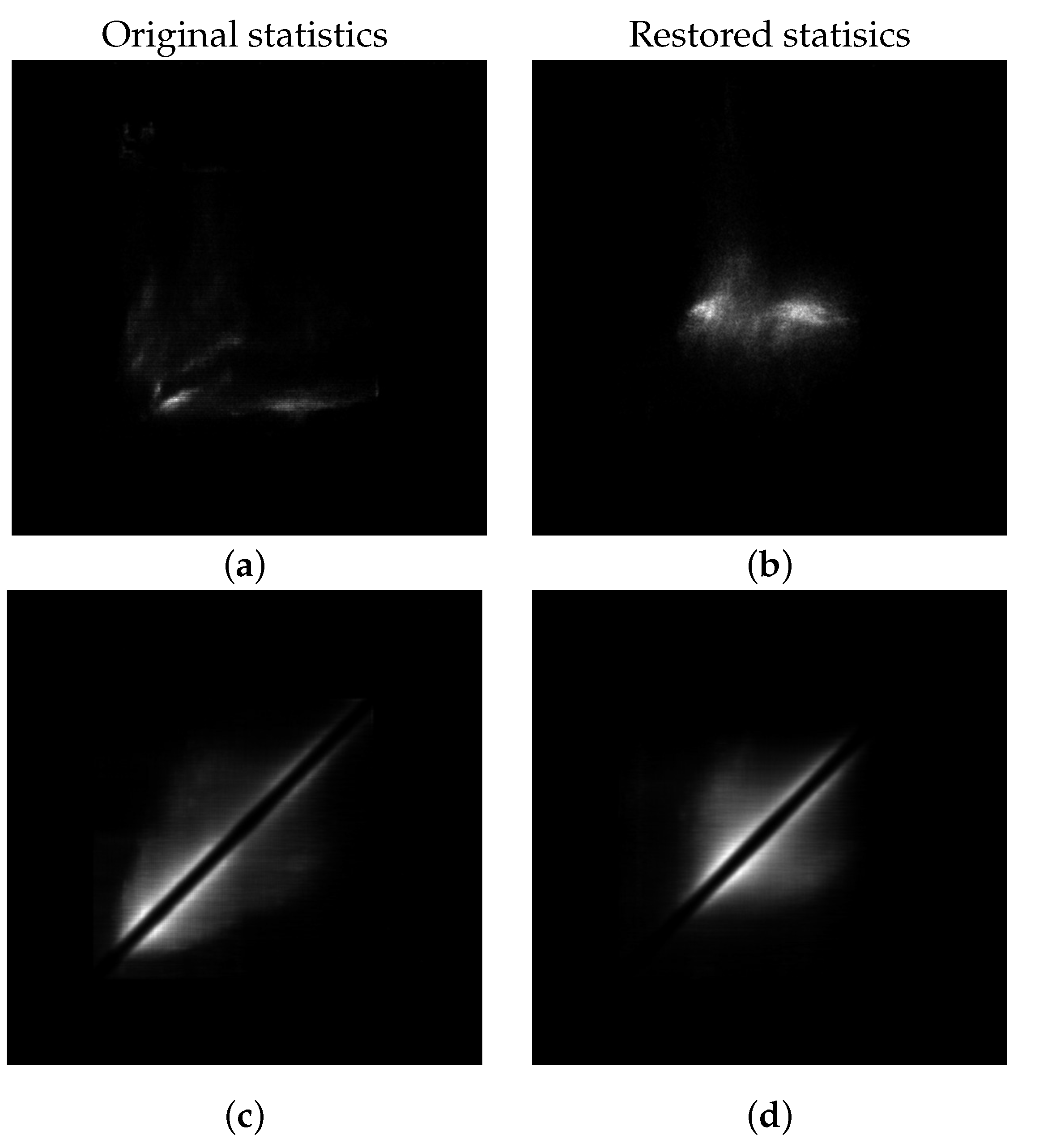
The images in Figure 2, Figure 3, Figure 4 and Figure 5 below offer representative examples of the processing of pairs of anatomic images, T 1 w TSE and T 1 w + T 2 w STIR, of two patients. The anatomic images for the first patient are presented in Figure 2 and the corresponding statistics are presented in Figure 3. The anatomic images for the second patient are presented in Figure 4 and the corresponding statistics are presented in Figure 5. The cumulative restoration fields in the second column of Figure 2 and Figure 4 represent the restorations for the intensity nonuniformities with their discontinuities. The third column of these figures shows the restored images. The restored statistics in the second column of Figure 3 and Figure 5 show that in the statistics of the restored images, the tissue distributions become sharper.
Figure 2. First example of joint restoration of T 1 w TSE and a T 1 w + T 2 w STIR. The cumulative restoration fields account for the spatial variations of the coil sensitivities, their different overall sensitivities, and the junctions between them. (a) Initial T 1 w image TSE; (b) Cumulative restoration field for TSE; (c) Restored T 1 w image TSE; (d) Initial T 1 w + T 2 w STIR image; (e) Cumulative restoration field for STIR; (f) Restored T 1 w + T 2 w STIR image.
Signals 04 00040 g002
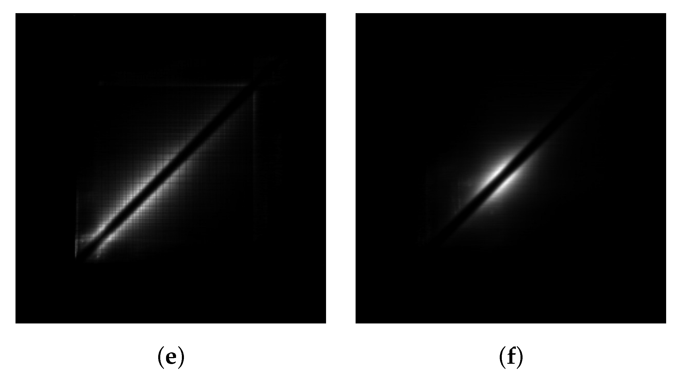
Figure 3. Co-Occurrence statistics of original and restored images of the first example in Figure 2. The restored statistics are sharper. The different distribution of the tissues are better shown in the restored joint-co-occurrence statistics in (b). (a) Original joint-co-occurrence statistics; (b) Restored joint-co-occurrence statistics; (c) Original T 1 w TSE co-occurrence statistics; (d) Restored T 1 w TSE co-occurrence statistics; (e) Original T 2 w STIR co-occurrence statistics; (f) Restored T 2 w STIR co-occurrence statistics.
Signals 04 00040 g003aSignals 04 00040 g003b
Figure 4. Second example of joint restoration of T 1 w TSE and a T 1 w + T 2 w STIR. The cumulative restoration fields account for the spatial variations of the coil sensitivities, their different overall sensitivities, and the junctions between them. (a) Initial T 1 w image TSE; (b) Cumulative restoration field for TSE; (c) Restored T 1 w image TSE; (d) Initial T 1 w + T 2 w STIR image; (e) Cumulative restoration field for STIR; (f) Restored T 1 w + T 2 w STIR image.
Signals 04 00040 g004aSignals 04 00040 g004b
Figure 5. Co-Occurrence statistics of original and restored images of the second example in Figure 4. The restored joint-co-occurrence statistics better show the distributions of the different tissues. The tissues distributions are shown improved in the restored co-occurrence statistics as well. (a) Original joint-co-occurrence statistics; (b) Restored joint-co-occurrence statistics; (c) Original T 1 w TSE co-occurrence statistics; (d) Restored T 1 w TSE co-occurrence statistics; (e) Original T 2 w STIR co-occurrence statistics; (f) Restored T 2 w STIR co-occurrence statistics.
Signals 04 00040 g005aSignals 04 00040 g005b
The measurement of improvement due to restoration uses the decrease in the value of the negative of the entropy of the statistics. In particular, the validation uses the negative of the entropy, H , of the joint-co-occurrence statistics. The initial entropy value is H 01 , i and the entropy of the final statistics is H 01 , f . In particular, the entropy ratio gain value is computed as
H r a t i o = e H 01 , f e H 01 , i e H 01 , i .
The method improves contrast in cases where H 01 , f < H 01 , i . This leads to H r a t i o < 0 and implies higher image quality. The statistics of the entropy ratio gain values over all images are presented in Table 2. The mean value, the minimum value, as well as the maximum value over all images are all negative. This shows that the method results in negative values for H r a t i o for all images. Hence, the method improves performance and is effective for all images.

5. Discussion and Conclusions

Whole-body MRI is a developing and promising imaging method that can be clinically useful for many purposes. It has found several novel applications and can potentially have even more applications. However, it still suffers from many acquisition artifacts. The restoration and the analysis of the MRI imaging data remains a challenge. One of the main artifacts decreasing data quality and preventing the understanding of the data is the intensity nonuniformities that can even have abrupt changes at the junctions between images corresponding to different coils. The proposed method addresses this problem by achieving homogenization of the intensities.
Statistical representation of the images involves co-occurrence statistics. The effect of using co-occurrences as opposed to plain intensity histograms is that they decrease the spread of the dominant distributions in the image and increase the contrasts between them. The sigmoid in the auto-co-occurrence statistics depresses the dominance of their diagonal that corresponds to the interior of intensity uniform image regions. Hence, the sigmoid increases the sensitivity to the statistics across region borders in the 2D statistical space. In whole-body images, the borders are from the extensive interface between not only different tissues, but also different organs as well. The assumed PSF of the distortion filter for the statistics is non-stationary and is used to design the deconvolution filter for the non-stationary restoration. The latter filter is, in turn, used to obtain the conditional expectation of the restored values.
The Bayesian estimate for the intensity correction is back-projected to the image to offer an initial rough estimate of intensity restoration. The Bayesian restoration is efficient since it computes and restores the co-occurrence statistics only once per iteration. The method is stable along the iterations and is even able to accommodate differences between the signal regions of the images.
The rough estimate of the restoration is smoothed with anisotropic Gaussian and anisotropic or inhomogeneous diffusion based on MDL that accommodates the discontinuities of the field at the junctions between images corresponding to different coils, and hence it is able to correct for nonuniformities. The junction surfaces between the images of the different coils may not be known a priori for an image and hence the method does not require their a priori knowledge. The anisotropic inhomogeneous diffusion method used represents the piecewise smooth regions of individual coils. There exists extensive literature on anisotropic image smoothing that preserves discontinuities. However, the methods in the literature are applied directly to the images. They can only accommodate pixel image noise and hence incorrectly interpret shades and discontinuities between the shades as being due to image structure [42,48]. This limitation of current methods is addressed in this work. It is able to account for sharp shading artifacts by applying the inhomogeneous diffusion to the spatial nonuniformity restoration field to estimate it.
The proposed methodology is also shown to be robust to the lower tissue quality of cancer patients data and the high-intensity distortions that are present in most images. The method also restores images effectively despite the more extensive and elongated whole-body anatomy compared to that of more traditional images of individual organs such as the brain which are typically processed for intensity nonuniformity restoration. To the authors’ knowledge, the proposed method can restore, for the first time, for intensity nonuniformities suffering from discontinuities in the context of MRI image processing. This method contributes to the restoration of datasets from whole-body imaging, which is an important and developing topic for several clinical applications.

Author Contributions

Conceptualization, S.H. and I.E.P.; Data curation, L.D.R. and I.E.P.; Methodology, S.H. and L.F.; Project administration, A.M.; Resources, L.D.R. and I.E.P.; Supervision, A.M. All authors have read and agreed to the published version of the manuscript.

Funding

This research received no external funding.

Institutional Review Board Statement

The data were analyzed retrospectively and fully anonymized in accordance with the ethical standards laid down in the 1964 Declaration of Helsinki and its amendments, the European Regulation 536/2014 and its latest addendum ICH GCP E6(R2)/2017, as well as with the guidelines of the Institutional Review Board (IRB) for clinical studies of the University of Jena (IRB number 2019-1452-Daten).

Data Availability Statement

The data presented in this study are available on request from the corresponding author and the authors that were responsible for data curation. The data are not publicly available due to privacy and ethical reasons.

Conflicts of Interest

The authors declare no conflict of interest.

Abbreviations

The following abbreviations are used in this manuscript:
PSFPoint Spread Function
RFRadio-Frequency
IRBInstitutional Review Board
T 1 w T 1 -weighted
T 2 w T 2 -weighted
WB-MRIWhole-Body Magnetic Resonance Imaging
RHSRight Hand Side
ICH GCPInternational Conference on Harmonization—Good Clinical Practice
TSETurbo Spin Echo
FFEFast Field Echo
STIRShort Tau Inversion Recovery
y.o.Years old
MDLMinimum Description Length
MAPMaximum A Posteriori

References

  1. Lecouvet, F.; Simon, M.; Tombal, B.; Jamart, J.; Vande Berg, B.C.; Simoni, P. Whole-body MRI (WB-MRI) versus axial skeleton MRI (AS-MRI) to detect and measure bone metastases in prostate cancer (PCa). Eur. Radiol. 2010, 20, 2973–2982. [Google Scholar] [CrossRef] [PubMed]
  2. Albano, D.; Cuocolo, R.; Patti, C.; Ugga, L.; Chianca, V.; Tarantino, V.; Faraone, R.; Albano, S.; Micci, G.; Costa, A.; et al. Whole-body MRI radiomics model to predict relapsed/refractory Hodgkin Lymphoma: A preliminary study. Magn. Reson. Imaging 2022, 86, 55–60. [Google Scholar] [CrossRef] [PubMed]
  3. Grueneisen, J.; Schaarschmidt, B.M.; Heubner, M.; Suntharalingam, S.; Milk, I.; Kinner, S.; Heubner, A.; Forsting, M.; Lauenstein, T.; Ruhlmann, V.; et al. Implementation of FAST-PET/MRI for whole-body staging of female patients with recurrent pelvic malignancies: A comparison to PET/CT. Eur. J. Radiol. 2015, 84, 2097–2102. [Google Scholar] [CrossRef]
  4. Petralia, G.; Zugni, F.; Summers, P.; Bellomi, M.; Petralia, G. Whole-body magnetic resonance imaging (WB-MRI) for cancer screening: Recommendations for use. Diagn. Imaging Oncol. 2021, 126, 1434–1450. [Google Scholar] [CrossRef]
  5. Thomas, E.; Fitzpatrick, J.; Malik, S.; Taylor-Robinson, S.; Bell, J. Whole body fat: Content and distribution. Prog. Nucl. Magn. Reson. Spectrosc. 2013, 73, 56–80. [Google Scholar] [CrossRef]
  6. Thomas, E.; Saeed, N.; Hajnal, J.; Brynes, A.; Goldstone, A.P.; Frost, G.; Bell, J.D. Magnetic resonance imaging of total body fat. J. Appl. Physiol. 1998, 85, 1778–1785. [Google Scholar] [CrossRef]
  7. Medina, T.; Kolb, J.; Hüttmann, G.; Huber, R.; Medina, O.; Ha, L.; Ulloa, P.; Larsen, N.; Ferrari, A.; Rafecas, M.; et al. Imaging Inflammation—From Whole Body Imaging to Cellular Resolution. Front. Immunol. 2021, 12, 692222. [Google Scholar] [CrossRef]
  8. Noterdaeme, O.; Brady, M. A Fast Method for Computing and Correcting Intensity Inhomogeneities in MRI. In Proceedings of the International Symposium on Biomedical Imaging (ISBI), Paris, France, 14–17 May 2008; pp. 1525–1528. [Google Scholar]
  9. Lui, D.; Modhafar, A.; Haider, M.; Wong, A. Monte Carlo-based Noise Compensation in Coil Intensity Corrected Endorectal MRI. BMC Med. Imaging 2015, 15. [Google Scholar] [CrossRef]
  10. Hooijmans, M.; Dzyubachyk, O.; Nehrke, K.; Koken, P.; Versluis, M.J.; Kan, H.E.; Börnert, P. Fast multistation water/fat imaging at 3T using DREAM-based RF shimming. J. Magn. Reson. Imaging 2015, 42, 217–223. [Google Scholar] [CrossRef]
  11. Zheng, Y.; Gee, J. Estimation of Image Bias Field with Sparsity Constraints. In Proceedings of the IEEE Computer Society Conference on Computer Vision and Pattern Recognition, San Francisco, CA, USA, 13–18 June 2010; pp. 255–262. [Google Scholar]
  12. Ma, W.; Morel, J.M.; Osher, S.; Chien, A. An L1-based variational model for Retinex theory and its application to medical images. In Proceedings of the Conference on Computer Vision and Pattern Recognition (CVPR), Colorado Springs, CO, USA, 20–25 June 2011; pp. 153–160. [Google Scholar] [CrossRef]
  13. Li, C.; Gore, J.; Davatzikos, C. Multiplicative intrinsic component optimization (MICO) for MRI bias field estimation and tissue segmentation. Magn. Reson. Imaging 2014, 32, 913–923. [Google Scholar] [CrossRef]
  14. Li, C.; Huang, R.; Ding, Z.; Gatenby, J.; Metaxas, D.; Gore, J. A Level Set Method for Image Segmentation in the Presence of Intensity Inhomogeneities With Application to MRI. IEEE Trans. Image Process. 2011, 20, 2007–2016. [Google Scholar] [PubMed]
  15. Zhang, H.; Ye, X.; Chen, Y. An Efficient Algorithm for Multiphase Image Segmentation with Intensity Bias Correction. IEEE Trans. Image Process. 2013, 22, 3842–3851. [Google Scholar] [CrossRef] [PubMed]
  16. Mangin, J. Entropy minimization for automatic correction of intensity nonuniformity. In Proceedings of the IEEE Workshop on MMBIA, Hilton Head, SC, USA, 12 June 2000; pp. 162–169. [Google Scholar]
  17. Simoncelli, E.; Adelson, E. Noise Removal via Bayesian Wavelet Coring. In Proceedings of the 3rd IEEE International Conference on Image Processing (ICIP), Lausanne, Switzerland, 16–19 September 1996; Volume 1, pp. 379–382. [Google Scholar]
  18. Vidal-Pantaleoni, A.; Martí, D. Comparison of different speckle reduction techniques in SAR images using wavelet transform. Int. J. Remote Sens. 2004, 25, 4915–4932. [Google Scholar] [CrossRef]
  19. Sled, J.; Zijdenbos, A.; Evans, A. A nonparametric method for automatic correction of intensity nonuniformity in MRI data. IEEE Trans. Med. Imaging 1998, 17, 87–97. [Google Scholar] [CrossRef]
  20. Renugadevi, M.; Varghese, D.; Vaithiyanathan, V.; Raju, N. Variational Level Set Segmentation and Bias Correction of Fused Medical Images. Asian J. Med. Sci. 2012, 4, 66–74. [Google Scholar]
  21. Fan, A.; Wells III, W.; Fisher III, J.; Cetin, M.; Haker, S.; Mulkern, R.; Tempany, C.; Willsky, A. A Unified Variational Approach to Denoising and Bias Correction in MR. In Information Processing in Medical Imaging, Proceedings of the 18th International Conference, IPMI 2003, Ambleside, UK, 20–25 July 2003; Springer: Berlin/Heidelberg, Germany, 2003; Volume 2732, pp. 148–159. [Google Scholar]
  22. Vovk, U.; Pernus, F.; Likar, B. Intensity inhomogeneity correction of multispectral MR images. Neuroimage 2006, 32, 54–61. [Google Scholar] [CrossRef]
  23. Miller, E.; Jain, V. Many heads are better than one: Jointly removing bias from multiple MRIs using nonparametric maximum likelihood. In Proceedings of the 19th International Conference on Information Processing in Medical Imaging, IPMI 2005, Glenwood Springs, CO, USA, 10–15 July 2005; Volume 3565, pp. 615–626. [Google Scholar]
  24. Iglesias, J.E.; Dinov, I.; Singh, J.; Tong, G.; Tu, Z. Synthetic MRI Signal Standardization: Application to Multi-atlas Analysis. In Proceedings of the Medical Image Computing and Computer-Assisted Intervention—MICCAI 2010, Beijing, China, 20–24 September 2010; Jiang, T., Navab, N., Pluim, J.P.W., Viergever, M.A., Eds.; Springer: Berlin/Heidelberg, Germany, 2010; Volume 6363, pp. 81–88. [Google Scholar]
  25. Jog, A.; Roy, S.; Carass, A.; Prince, J. Pulse sequence based multi-acquisition MR intensity normalization. In Proceedings of the Medical Imaging 2013: Image Processing, Lake Buena Vista, FL, USA, 9–14 February 2013; Ourselin, S., Haynor, D.R., Eds.; International Society for Optics and Photonics, SPIE: Bellingham, WA, USA, 2013; Volume 8669, p. 86692H. [Google Scholar] [CrossRef]
  26. Nyul, L.; Udupa, J. On standardizing the MR image intensity scale. Magn. Reson. Med. 1999, 42, 1072–1081. [Google Scholar] [CrossRef]
  27. Schmidt, M. A Method for Standardizing MR Intensities between Slices and Volumes; Technical Report, TR05-14; University of Alberta: Edmonton, AB, Canada, 2005. [Google Scholar] [CrossRef]
  28. Weisenfeld, N.; Warfield, S. Normalization of joint image-intensity statistics in MRI using the Kullback-Leibler divergence. In Proceedings of the 2004 2nd IEEE International Symposium on Biomedical Imaging: Nano to Macro (IEEE Cat No. 04EX821), Arlington, VA, USA, 15–18 April 2004; Volume 1, pp. 101–104. [Google Scholar] [CrossRef]
  29. Bergeest, J.P.; Jäger, F. A Comparison of Five Methods for Signal Intensity Standardization in MRI. In Proceedings of the Bildverarbeitung für die Medizin 2008, Berlin, Germany, 6–8 April 2008; Tolxdorff, T., Braun, J., Deserno, T.M., Horsch, A., Handels, H., Meinzer, H.P., Eds.; Springer: Berlin/Heidelberg, Germany, 2008; pp. 36–40. [Google Scholar]
  30. Madabhushi, A.; Udupa, J. Interplay between intensity standardization and inhomogeneity correction in MR image processing. IEEE Trans. Med. Imaging 2005, 24, 561–576. [Google Scholar] [CrossRef]
  31. Robinson, K.; Ghita, O.; Whelan, P.F. Intensity non-uniformity correction in multi-section whole body MRI. In Proceedings of the Opto-Ireland 2005: Imaging and Vision, Dublin, Ireland, 5–6 April 2005; Murtagh, F.D., Ed.; International Society for Optics and Photonics, SPIE: Bellingham, WA, USA, 2005; Volume 5823, pp. 164–174. [Google Scholar] [CrossRef]
  32. Jäger, F.; Nyúl, L.; Frericks, B.; Wacker, F.; Hornegger, J. Whole Body MRI Intensity Standardization. In Proceedings of the Bildverarbeitung für die Medizin 2007, Munich, Germany, 25–27 March 2007; Horsch, A., Deserno, T.M., Handels, H., Meinzer, H.P., Tolxdorff, T., Eds.; Springer: Berlin/Heidelberg, Germany, 2007; pp. 459–463. [Google Scholar]
  33. Jager, F.; Hornegger, J. Nonrigid Registration of Joint Histograms for Intensity Standardization in Magnetic Resonance Imaging. IEEE Trans. Med. Imaging 2009, 28, 137–150. [Google Scholar] [CrossRef]
  34. Li, C.; Xu, C.; Anderson, A.; Gore, J. MRI Tissue Classification and Bias Field Estimation Based on Coherent Local Intensity Clustering: A Unified Energy Minimization Framework. In Proceedings of the International Conference on Information Processing in Medical Imaging IPMI 2009, Williamsburg, VA, USA, 5–10 July 2009; Volume 5636, pp. 288–299. [Google Scholar]
  35. Dzyubachyk, O.; van der Geest, R.J.; Staring, M.; Börnert, P.; Reijnierse, M.; Bloem, J.L.; Lelieveldt, B.P.F. Joint Intensity Inhomogeneity Correction for Whole-Body MR Data. In Proceedings of the Medical Image Computing and Computer-Assisted Intervention—MICCAI 2013, Nagoya, Japan, 22–26 September 2013; Mori, K., Sakuma, I., Sato, Y., Barillot, C., Navab, N., Eds.; Springer: Berlin/Heidelberg, Germany, 2013; Volume 8149, pp. 106–113. [Google Scholar]
  36. Tustison, N.; Avants, B.; Cook, P.; Zheng, Y.; Egan, A.; Yushkevich, P.; Gee, J. N4ITK: Improved N3 Bias Correction. IEEE Trans. Med. Imaging 2010, 29, 1310–1320. [Google Scholar] [CrossRef]
  37. Dzyubachyk, O.; Staring, M.; Reijnierse, M.; Lelieveldt, B.; Geest, R. Inter-station intensity standardization for whole-body MR data. Magn. Reson. Med. 2016, 77, 422–433. [Google Scholar] [CrossRef]
  38. Perona, P.; Malik, J. Scale-space and edge detection using anisotropic diffusion. IEEE Trans. Pattern Anal. Mach. Intell. 1990, 12, 629–639. [Google Scholar] [CrossRef]
  39. Sapiro, G. Geometric Partial Differential Equations and Image Analysis; Cambridge University Press: Cambridge, UK, 2001. [Google Scholar]
  40. Sapiro, G. Geometric partial differential equations in image analysis: Past, present, and future. In Proceedings of the International Conference on Image Processing, 1995, Washington, DC, USA, 23–26 October 1995; Volume 3, pp. 1–4. [Google Scholar] [CrossRef]
  41. Leclerc, Y. Constructing simple stable descriptions for image partitioning. Int. J. Comput. Vis. 1989, 3, 73–102. [Google Scholar] [CrossRef]
  42. Leclerc, Y. The Local Structure of Image Intensity Discontinuities; McGill University: Montreal, QC, Canada, 1989. [Google Scholar]
  43. Yue, H.; Yang, J.; Sun, X.; Wu, F.; Hou, C. Contrast Enhancement Based on Intrinsic Image Decomposition. IEEE Trans. Image Process. 2017, 26, 3981–3994. [Google Scholar] [CrossRef]
  44. Bi, S.; Han, X.; Yu, Y. An L1 image transform for edge-preserving smoothing and scene-level intrinsic decomposition. ACM Trans. Graph. 2015, 34, 1–12. [Google Scholar] [CrossRef]
  45. Cai, J.F.; Dong, B.; Shen, Z. Image restoration: A wavelet frame based model for piecewise smooth functions and beyond. Sparse Representations with Applications in Imaging Science, Data Analysis and Beyond. Appl. Comput. Harmon. Anal. 2016, 41, 94–138. [Google Scholar] [CrossRef]
  46. Trzasko, J.; Manduca, A. Highly Undersampled Magnetic Resonance Image Reconstruction via Homotopic 0 -Minimization. IEEE Trans. Med. Imaging 2009, 28, 106–121. [Google Scholar] [CrossRef]
  47. Krissian, K.; Aja-Fernandez, S. Noise-Driven Anisotropic Diffusion Filtering of MRI. IEEE Trans. Image Process. 2009, 18, 2265–2274. [Google Scholar] [CrossRef]
  48. Leclerc, Y.G.; Zucker, S.W. The Local Structure of Image Discontinuities in One Dimension. IEEE Trans. Pattern Anal. Mach. Intell. 1987, PAMI-9, 341–355. [Google Scholar] [CrossRef]
  49. Hadjidemetriou, S.; Studholme, C.; Mueller, S.; Weiner, M.; Schuff, N. Restoration of MRI data for intensity non-uniformities using local high order intensity statistics. Med. Image Anal. 2009, 13, 36–48. [Google Scholar] [CrossRef]
  50. Hadjidemetriou, S.; Buechert, M.; Ludwig, U.; Hennig, J. Joint Restoration of Bi-contrast MRI Data for Spatial Intensity Non-uniformities. In Information Processing in Medical Imaging, Proceedings of the 22nd International Conference, IPMI 2011, Kloster Irsee, Germany, 3–8 July 2011; Springer: Berlin/Heidelberg, Germany, 2011; Volume 6801, pp. 346–358. [Google Scholar]
  51. Hadjidemetriou, S.; Psychogios, M.N.; Lingor, P.; Von Eckardstein, K.; Papageorgiou, I. Restoration of Bi-Contrast MRI Data for Intensity Uniformity with Bayesian Coring of Co-Occurrence Statistics. J. Imaging 2017, 3, 67. [Google Scholar] [CrossRef]
  52. Hadjidemetriou, S.; Psychogios, M.N.; Lingor, P.; von Eckardstein, K.; Papageorgiou, I. Restoration of Intensity Uniformity of Bi-contrast MRI Data with Bayesian Co-Occurrence Coring. In Proceedings of the Medical Image Understanding and Analysis—21st Annual Conference, MIUA 2017, Edinburgh, UK, 11–13 July 2017; del C. Valdés Hernández, M., González-Castro, V., Eds.; Springer: Berlin/Heidelberg, Germany, 2017; Volume 723, pp. 616–628. [Google Scholar] [CrossRef]
  53. Papageorgiou, I.; Dvorak, J.; Cosma, I.; Pfeil, A.; Teichgraeber, U.; Malich, A. Whole-body MRI: A powerful alternative to bone scan for bone marrow staging without radiation and gadolinium enhancer. Clin. Transl. Oncol. 2019, 22, 1321–1328. [Google Scholar] [CrossRef] [PubMed]
  54. Bennia, A.; Riad, S. Filtering Capabilities and Convergence of the Van-Cittert Deconvolution Technique. IEEE Trans. Instrum. Meas. 1992, 41, 246–250. [Google Scholar] [CrossRef]
  55. Otsu, N. A Threshold Selection Method from Gray-Level Histograms. IEEE Trans. Syst. Man. Cybern. 1979, 9, 62–66. [Google Scholar] [CrossRef]
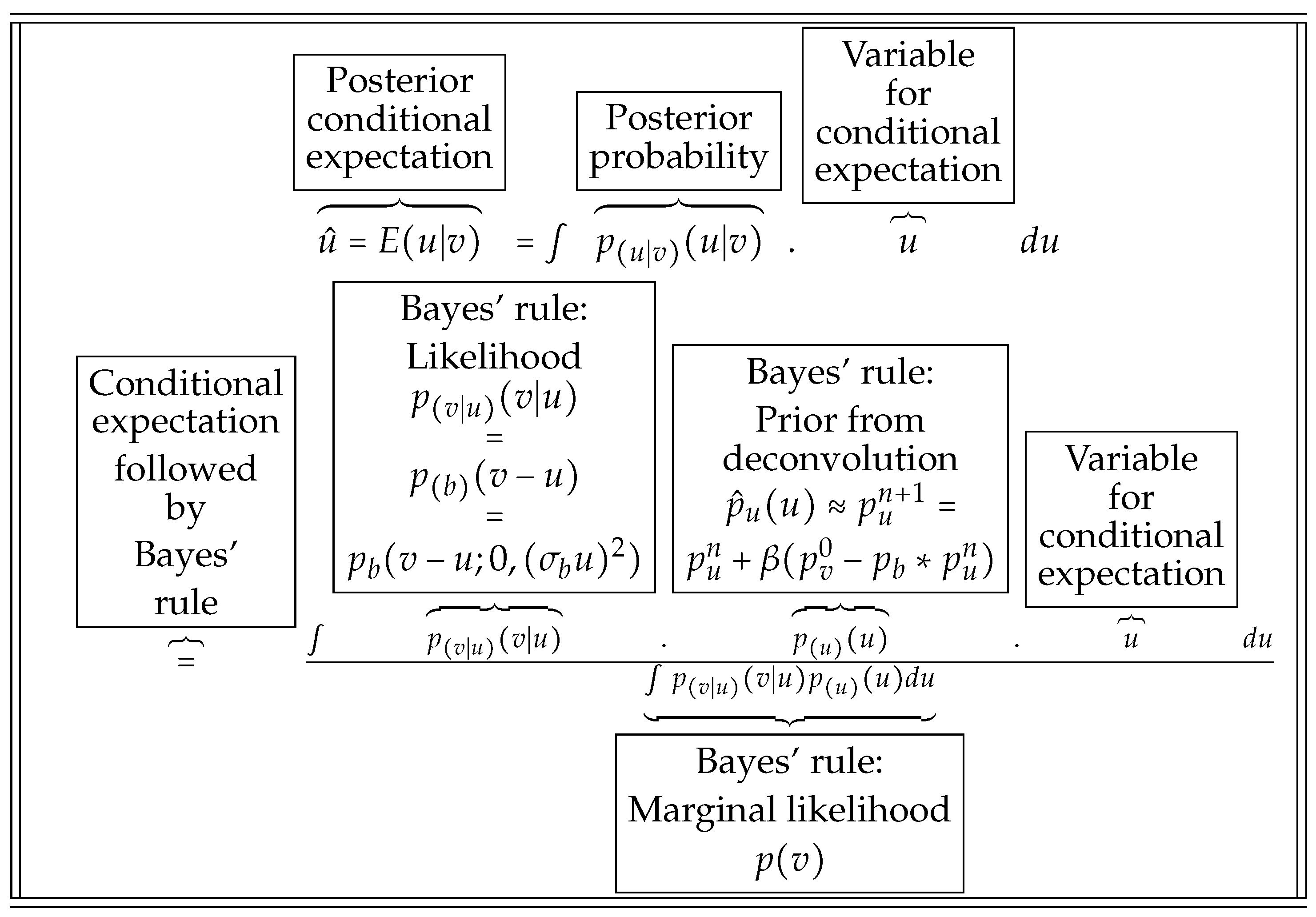
Figure 1. Overview of the non-parametric Bayesian coring derivation of the posterior conditional expectation. The conditional expectation is further expanded with Bayes’ rule. The expressions for the prior and the likelihood are then substituted. It provides the intermediate vector field u ^ = E ( u | v , x ) for image restoration.
Signals 04 00040 g001
Table 1. Acquisition parameters of the imaging sequences for individual coils.
Parameters ∖Sequence,
Static Field
T 1 w TSE
1.5 T
STIR
1.5 T
T 1 w TSE
3.0 T
STIR
3.0 T
Number of
slices
66666060
Voxel size
mm2
1.17 × 1.17 0.95 × 0.95 1.02 × 1.02 1.04 × 1.04
Slice hickness
(mm)
3333
Spacing
(slice gap) (mm)
0.30.311
Matrix
size
215 × 188 226 × 152 233 × 180 151 × 148
Table 2. Statistics of entropy ratio gain values H r a t i o for validation.
MeanSt.Dev.MedianMinimumMaximum
−0.460.23−0.52−0.89−0.02
Disclaimer/Publisher’s Note: The statements, opinions and data contained in all publications are solely those of the individual author(s) and contributor(s) and not of MDPI and/or the editor(s). MDPI and/or the editor(s) disclaim responsibility for any injury to people or property resulting from any ideas, methods, instructions or products referred to in the content.