Abstract
The goal of this study is to explore the effectiveness of applying multi-objective particle swarm optimization (MOPSO) algorithms in the design of infinite impulse response (IIR) filters. Given the widespread application of IIR filters in digital signal processing, the precision of their design plays a significant role in the system’s performance. Traditional design methods often encounter the problem of local optima, which limits further enhancement of the filter’s performance. This research proposes a method based on multi-objective particle swarm optimization algorithms, aiming not just to find the local optima but to identify the optimal global design parameters for the filters. The design methodology section will provide a detailed introduction to the application of multi-objective particle swarm optimization algorithms in the IIR filter design process, including particle initialization, velocity and position updates, and the definition of objective functions. Through multiple experiments using Butterworth and Chebyshev Type I filters as prototypes, as well as examining the differences in the performance among these filters in low-pass, high-pass, and band-pass configurations, this study compares their efficiencies. The minimum mean square error (MMSE) of this study reached 1.83, the mean error (ME) reached 2.34, and the standard deviation (SD) reached 0.03, which is better than the references. In summary, this research demonstrates that multi-objective particle swarm optimization algorithms are an effective and practical approach in the design of IIR filters.
1. Introduction
Digital signal processing (DSP) plays a crucial role in contemporary technology, including in communication systems, audio signal processing, image processing, and medical applications [1,2,3]. Infinite impulse response (IIR) filters, as fundamental components in DSP, have a direct impact on the overall system performance. Whether implemented in hardware or software, the design of IIR filters significantly influences the results achieved. In designing IIR filters, challenges such as selecting design parameters, ensuring filter stability, and meeting specific frequency response requirements must be addressed. Traditional design methods like the bilinear transform method [4] or frequency sampling method [5,6,7,8,9] are often limited when facing complex filter specifications. These methods might not achieve optimal design, especially in cases requiring precise control over filter characteristics or in handling complex requirements, potentially leading to issues like instability, distortion, or ineffective noise reduction. These methods also require extensive manual adjustment and testing, making the design process tedious and inflexible. To overcome these issues, particle swarm optimization (PSO) or multi-objective particle swarm optimization (MOPSO) can be used. Although MOPSO is used to design filters [10], this article discusses how to design hardware components such as capacitors and resistors for analog filters while focusing designing digital filters, and at the same time using Pareto efficiency combined with MOPSO rules to design parameters related to digital filters. By setting target functions, these algorithms help achieve the best design parameters for filters. PSO, a group intelligence-based optimization method, has proven effective in various domains for solving complex problems, offering a new approach to overcome the limitations of traditional IIR filter design methods. Its advantages include simplicity, ease of implementation, and excellent global optimization capabilities, making PSO a compelling choice for traditional IIR filter design issues. Combining PSO with IIR filter design through automated optimization processes not only enhances design efficiency and accuracy but also explores new filter design methods, providing precise and efficient signal processing solutions for complex systems. The successful application of this method also promotes further research and application of PSO and other evolutionary algorithms in the field of signal processing. Haruna Aimi and Kenji Suyama [11] propose a novel approach utilizing a multi-swarm PSO framework to reallocate particles dynamically, using the global bests from multiple swarms to define a new search space. Kenzo Yamamoto and Kenji Suyama [12] propose addressing local minimum stagnation in traditional PSO approaches to IIR filter design by implementing a fixed penalty range and alternating between diversification and intensification strategies. G. Dhanarasi et al. [13] aim to design an optimal stable digital low pass IIR filter using a modified particle swarm optimization approach, incorporating a constriction factor and inertia weight approach (PSO-CFIWA). This method is intended to overcome the limitations of standard PSO, such as premature convergence and stagnation, by adjusting the particle velocities more effectively during the search process. Yuya Takase and Kenji Suyama [14] aim to enhance the PSO method to overcome the drawback of premature convergence by incorporating a diversification strategy called Problem Space Stretch (PSS)-PSO. This approach modifies the search space dynamically to avoid local minima stagnation, allowing for a more thorough exploration of the solution space. This study explores the application of particle swarm optimization in IIR filter design, evaluating the effectiveness of MOPSO in optimizing IIR filter design parameters, including stability, frequency response, and phase response. MOPSO simplifies the IIR filter design process, reduces complexity, improves efficiency, and explores the possibilities of automated filter design. The adaptability of MOPSO in handling multi-variable optimization problems, especially in designing IIR filters with specific performance requirements like minimizing passband and stopband errors or optimizing transition bandwidth, is also assessed. Furthermore, the application of MOPSO in various types of IIR filter designs, such as low-pass, high-pass, and band-pass filters or more complex designs, is explored. This study demonstrates MOPSO’s effectiveness in finding global optimal solutions for IIR filters, particularly in overcoming the issues of traditional methods that often get stuck in local optima. These research objectives provide a deep understanding of the potential and challenges of multi-objective particle swarm optimization in IIR filter design, offering valuable insights and methodologies to advance the technology in the digital signal processing field.
The structure of this paper is as follows: Section 2 details the methodologies and system description, and Section 3 shows the experimental results. In Section 4 and Section 5, the experimental results are discussed, and the main findings and contributions of this study are summarized, respectively.
2. Methodologies and System Description
This research will use the Butterworth filter and Chebyshev filter as prototypes, conduct particle swarm optimization and Pareto efficiency to achieve multi-objective optimized filter design parameters, and design the filter design parameters through the obtained optimal design parameters. Low-pass, high-pass, and band-pass filters complying with Butterworth and Chebyshev Type I theorems are presented below.
2.1. Low-Pass Filter
A low-pass filter is designed to only allow signals with frequencies below a specific cutoff frequency to pass through. When designing an IIR low-pass filter, key design parameters include cutoff frequency, filter order, and transfer function. The transfer function and difference equation [15] are Equations (1) and (2), respectively, essential mathematical formulas for designing IIR low-pass filters.
2.2. High-Pass Filter
A high-pass filter allows frequency components above a specific cutoff frequency while suppressing those below that. In addition to the basic mathematical formulas mentioned earlier, the design of IIR high-pass filters also incorporates other important mathematical concepts and formulas [15], such as the Frequency Conversion of Equation (3); a standard method uses frequency transformation formulas to convert low-pass filters into high-pass filters.
Alternatively, Equation (4) of group delay is used. Group delay measures how a filter’s phase response changes with frequency, indicating the filter’s delay for different frequency components.
2.3. Band-Pass Filter
The core of a band-pass filter is also represented through mathematical formulas like transfer functions and difference equations, as mentioned in Section 2.1. The frequency response of a band-pass filter is a crucial characteristic that describes how the filter affects the amplitude of signals at different frequencies.
However, a band-pass filter focuses explicitly on two frequency points: the lower cutoff frequency and the upper cutoff frequency . The design aims to allow signals within these frequency ranges to pass through while attenuating signals outside this range. The filter’s bandwidth () is given by Equation (5), and the center frequency () is given by Equation (6) [15].
2.4. Butterworth Filter
The Butterworth filter, known for its unique design and performance characteristics, has a maximally flat frequency response in the passband, meaning there are no ripples. Its crucial feature is achieving a smooth response across the entire passband by eliminating ripples, ensuring signal stability and predictability. The characteristics of this filter can be primarily divided into the following three aspects.
- Maximal Flatness
The frequency response of a Butterworth filter in the passband is flat, with no ripples. This means all frequencies passing through have the same gain, ensuring stable signal transmission.
- 2.
- Transition Band Performance
Its transition band is smooth but less steep than Chebyshev or elliptical filters. This ensures the Butterworth filter provides gradual and smooth control in the transition band, preventing sudden changes to the signal.
- 3.
- Flexible Order Design
The Butterworth filter can be designed to any order. Higher orders lead to steeper transitions between the passband and stopband but can result in increased phase distortion.
Various mathematical formulas, such as the transfer function and frequency response, can be used to design and analyze a Butterworth filter, for example, the Transfer Function of Equation (7) [15].
- is a complex frequency variable (i.e., Laplacian variable), is the angular frequency. is the cutoff frequency. is the order of the filter. G is the gain, usually set to 1, so that when , the value of is .
2.5. Chebyshev Filter
An equiripple response in either the passband or the stopband characterizes the Chebyshev filter. Compared to the Butterworth filter, this filter provides a steeper transition in the transition band at the cost of introducing ripples in the passband or stopband. Chebyshev filters are categorized into two types based on their ripple characteristics.
- Type I Chebyshev Filter
This filter has equal ripples in the passband and remains flat in the stopband. This design suits applications that can tolerate passband oscillation but require high stopband attenuation.
- 2.
- Type II Chebyshev Filter
This kind of filter is also called an inverse Chebyshev filter. It has equal ripples in the stop band and remains flat in the pass band. It is suitable for situations where a stable response needs to be maintained in the pass band.
Chebyshev filters can be designed using mathematical formulas such as transfer functions, polynomials, and others [15]. The transfer functions are expressed as in Equations (8) and (9), respectively.
- Equations (8) and (9) are only true when , is the ripple coefficient, is the cutoff frequency, and is the order of the filter. is a Chebyshev polynomial of type I, and is a Chebyshev polynomial of type II.
2.6. Particle Swarm Optimization (PSO) Algorithm
In the particle swarm optimization algorithm, “particles” refer to the abstract representation of potential solutions. Each particle has its position and speed. These particles are randomly placed in the multi-dimensional search space. Each particle represents the search A point in space, which is a possible solution, and the “speed” of the particle determines its movement direction and distance in the search space [16,17,18,19,20].
Particle position update is the core concept in the particle swarm optimization algorithm. Each particle swarm updates its speed and position based on its own flight experience and the experience of other particles in the group. Specifically, the particle speed update considers three factors: the current speed, the best position found by the particle so far (pbest), and the best position found by all particles in the group (gbest). This update mechanism facilitates both local search (via pbest) and global search (via gbest), thus balancing the needs of exploration and exploitation.
To improve the efficiency of the algorithm and avoid premature convergence, subsequent research introduced the concept of inertia weight. Inertia weight controls the degree of retention of particle speed and helps particles balance between global exploration and local exploration. By adjusting the inertia weight, extensive exploration and detailed local exploration of the solution space can be promoted at different stages of the algorithm; the performance of the particle swarm optimization algorithm depends to a large extent on the selection of parameters, including the size of the particle swarm, inertial weights and learning factors that control the social behavior of particles (i.e., pbest and gbest effects). The selection of these parameters must be adjusted according to the specific problem to achieve the best performance.
The main calculation formulas involved in the particle swarm optimization algorithm include particle speed update and position update. These formulas are the algorithm’s core and are used to simulate the exploration behavior of particles in the solution space. Formulas (10)–(12) are particle speed update, position update, and dynamic adjustment of all tank types.
- is the velocity of particle at the next time step.
- is the inertia weight, which controls the degree of retention of particle speed.
- is the speed of particle i at the current time step.
- and are learning factors, which are called personal learning factors and social learning factors, respectively. They are used to adjust the tendency of particles to move to pbest and gbest.
- and are random numbers in the range [0, 1], used to introduce randomness.
- is the best position found so far for particle , and is the best position found by all particles in the swarm.
- is the position of particle i at the current time step, and is the position of particle i at the next time step.
- is the maximum value of the inertia weight, and is the minimum value of the inertia weight.
- is the current iteration number, and is the maximum number of iterations.
2.7. Multi-Objective Particle Swarm Optimization (MOPSO) Algorithm
MOPSO is widely used in engineering, economics, science, and other fields. The difference between MOPSO and PSO is that PSO is used to find a single best solution with a single objective function, while MOPSO uses multiple objective functions to find a set of solutions. In this case, the objectives are usually conflicting with each other; so, it is necessary to seek a set of equilibrium solutions to handle multi-objective optimization problems by introducing external files and domination sorting. In order to effectively handle multi-objective optimization problems, some specific strategies need to be introduced to ensure that well-diversified and evenly distributed Pareto fronts are found. These strategies include the following:
- External Archive
The external archive is used to store the non-dominated solutions found so far. The external archive usually has a fixed size and needs to be updated regularly to maintain its diversity and representativeness. When the size of the external archive exceeds the predetermined capacity, strategies such as fitness will be used. Ranking or diffusion distance are used to select which solutions to retain, ensuring the solution set’s diversity.
- 2.
- Selection of Guide Particles
When updating the particle speed, a non-dominated solution is selected from the external file as the particle’s reference (guide) particle. It can be selected randomly or based on specific criteria (such as fit, distance, etc.). The purpose is to promote search diversity and distribution uniformity.
- 3.
- Fitness Assessment and Dominance Judgment
Each particle calculates its fitness based on the values of all objective functions to determine whether each particle is dominated by other particles (that is, it is not inferior to another particle on all objectives and is better than another particle on at least one objective).
- 4.
- Archive Update Strategy
After each generation iteration, the new non-dominated solutions are merged with the external archive, and then the optimal solution is retained according to the reduction strategy. Strategies such as fitness ranking, or diffusion distance ensure that the solutions in the archive are evenly distributed in the target space.
- 5.
- Distance Measure and Goodness of Fit Ranking
Crowding distance measures the crowding degree of solutions in the target space and prioritizes retaining solutions with lower crowding degrees to ensure the uniformity of distribution of the Pareto front. Fitness assignment assigns a fitness value to each particle based on the particle’s dominance relationship and distance measurement for selection and update.
2.8. Pareto Efficiency
Pareto efficiency provides a framework to help solve these multi-objective optimization problems. Pareto efficiency focuses on finding solutions that can do better on all objectives simultaneously when no other solution can. In the best case, the best at some goal, these solutions form the Pareto Front, representing the best trade-offs between different design choices.
When implementing multi-objective optimization, engineers often use various algorithms, such as Genetic Algorithm (GA) [21] and multi-objective particle swarm optimization algorithm [22], to explore the possible design space and find the Paley owing to the cutting edge. These algorithms can effectively identify balanced solutions across all objectives considered. In multi-objective optimization problems in engineering and economics, the goal is to maximize or minimize multiple objective functions simultaneously. These problems can be expressed as follows:
are the objective functions, is the constraint of the inequality, and is the constraint of Equation, the vector of decision variables.
2.9. Particle Swarm Algorithm Combined with Pareto Efficiency Process
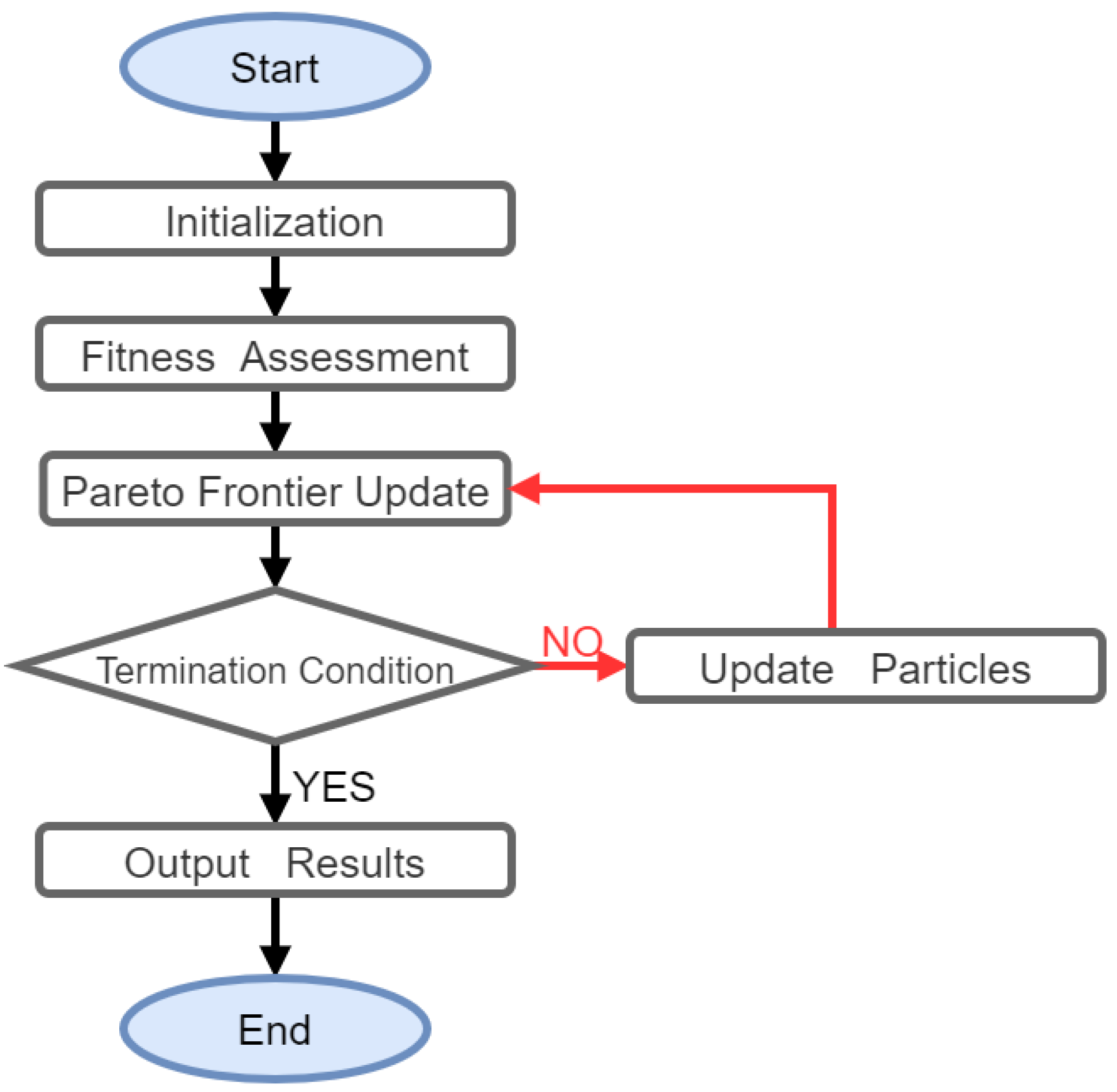
Table 1 shows the multi-objective particle swarm optimization algorithm parameters for MOPSO. Figure 1 shows a flow chart of the PSO algorithm combined with Pareto efficiency to form a MOPSO algorithm. It starts at random by generating a group of particles and initializing them. Next, the fitness value of each example according to the multi-objective function is evaluated, and the individual and global optimal solutions are updated based on the Pareto dominance rule. The particle updates its position and velocity based on these optimal solutions while updating the Pareto front to reflect the best non-dominated solution found. Finally, this process is repeated until the termination condition is met. The objective function can be changed according to the type of filter to be designed. And the fitness function of MOPSO can be expressed in the following mathematical form:

Table 1.
MOPSO algorithm parameter settings.
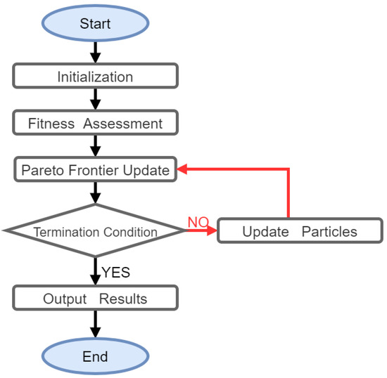
Figure 1.
PSO algorithm combined with Pareto efficiency process.
Among them, can represent the passband oscillation, can represent the stopband suppression, can represent the range of the numerator or denominator coefficient of the filter, and can be increased or decreased according to the set parameters. is the parameter vector of the particle.
In Pareto efficiency, target constraints and correction sorting mechanisms are added. The concept of objective constraints is to transform specific objectives into constraints and optimize other objectives only under these constraints. For example, a threshold for a specific goal can be set, and only when this threshold is met will the optimization of other goals be considered, which can be expressed by a mathematical formula (17). The concept of modifying the ranking is to introduce additional ranking criteria. For example, Pareto ranking can be adjusted based on the distribution, uniformity, or diversity of solutions to ensure the diversity of solutions and the uniformity of distribution.
Among them, is the preset constraint threshold.
The following is the pseudocode architecture process of proposal method.
Pseudocode steps:
Define fitness_function(x):
Define objective_constraints(f1, f2, f3, …, fn):
Initialize_particles(num_particles, dim):
Update_particles(particles, velocities, p_best, g_best, w, c1, c2):
Pareto_sort(particles, fitness_values):
MOPSO_algorithm(num_particles, dim, num_iterations, w, c1, c2):
|
- Define fitness_function(x).
- Define objective_constraints(f1, f2, f3, …, fn).
- Initialize particles using Initialize_particles(num_particles, dim).
- For each iteration from 1 to num_iterations:
- Calculate fitness values for each particle using fitness_function.
- Update personal best positions (p_best) and fitness values (p_best_fitness), If current fitness values are better than personal best values.
- Use Pareto_sort to get Pareto front indices.
- Update global best position (g_best) to the best solution in Pareto front.
- Output the best particle position (g_best) and the best particle fitness values (g_best_fitness).
2.10. Experimental Procedure
Figure 2 shows a flow chart of the experimental steps used in this experiment to apply the MOPSO algorithm to the design of IIR filters. This experimental step can be divided into parameter setting, MOPSO optimization, and filter design.
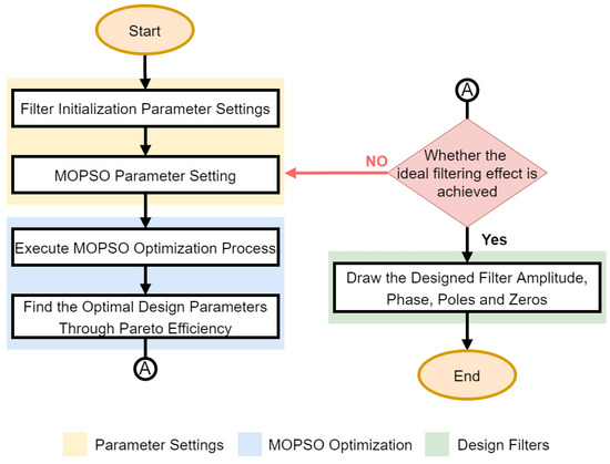
Figure 2.
Design system process diagram of MOPSO algorithm applied to IIR Filter.
- Parameter Setting: In the initial basic parameter settings, we first need to set the filter type to be optimized and the filter type, such as low-pass, high-pass, band-pass, and other filter types. The initial filter parameter settings also include filter sampling. Frequency, passband frequency range, stopband frequency range, and frequency response; MOPSO initial parameter settings include objective function, number of iterations, number of particles, weights, and other related parameters; this study uses Butterworth filter, and two types of Chebyshev Type I filters as prototypes, and the design parameters of these two types of low-pass filters, high-pass filters, and band-pass filters are optimized.
- MOPSO Optimization: The MOPSO optimization algorithm is used to form a Pareto boundary for each set of iterated solutions and find a set of relatively optimal trade-off solutions through Pareto efficiency. All relevant constraints are defined according to the type of filter to be designed. Each candidate solution should be a vector containing the values of all objective functions. An external archive is used to store the Pareto optimal solution set (Pareto front). The solution of the current particle is compared with the solution in the Pareto Archive, and the archive is updated to keep it containing only non-dominated solutions (Pareto optimal solutions) until the stopping condition is met (for example, the maximum number of iterations is reached, or the solution no longer changes significantly in the external archive). Return to the parameter-setting part if the ideal filtering effect is not achieved and readjust parameters.
- Design Filter: The obtained optimal design parameter solution is used to design a filter and draw the filter amplitude, phase, pole, and zero-point diagrams; then, a section of white noise is randomly generated and filtered through the designed filter. Moreover, the signal-to-noise ratio (SNR) before and after filtering is calculated to confirm whether the designed filter achieves the filtering effect.
3. Experimental Results
In this experiment, the Butterworth filter and Chebyshev Type I filter were used as design prototypes to optimize low-pass, high-pass, and band-pass filters that meet the characteristics, and white noise was randomly generated and filtered through the filter. After calculating the SNR before and after filtering, it is confirmed that the design parameters optimized through the MOPSO algorithm can effectively improve the filter performance.
Results
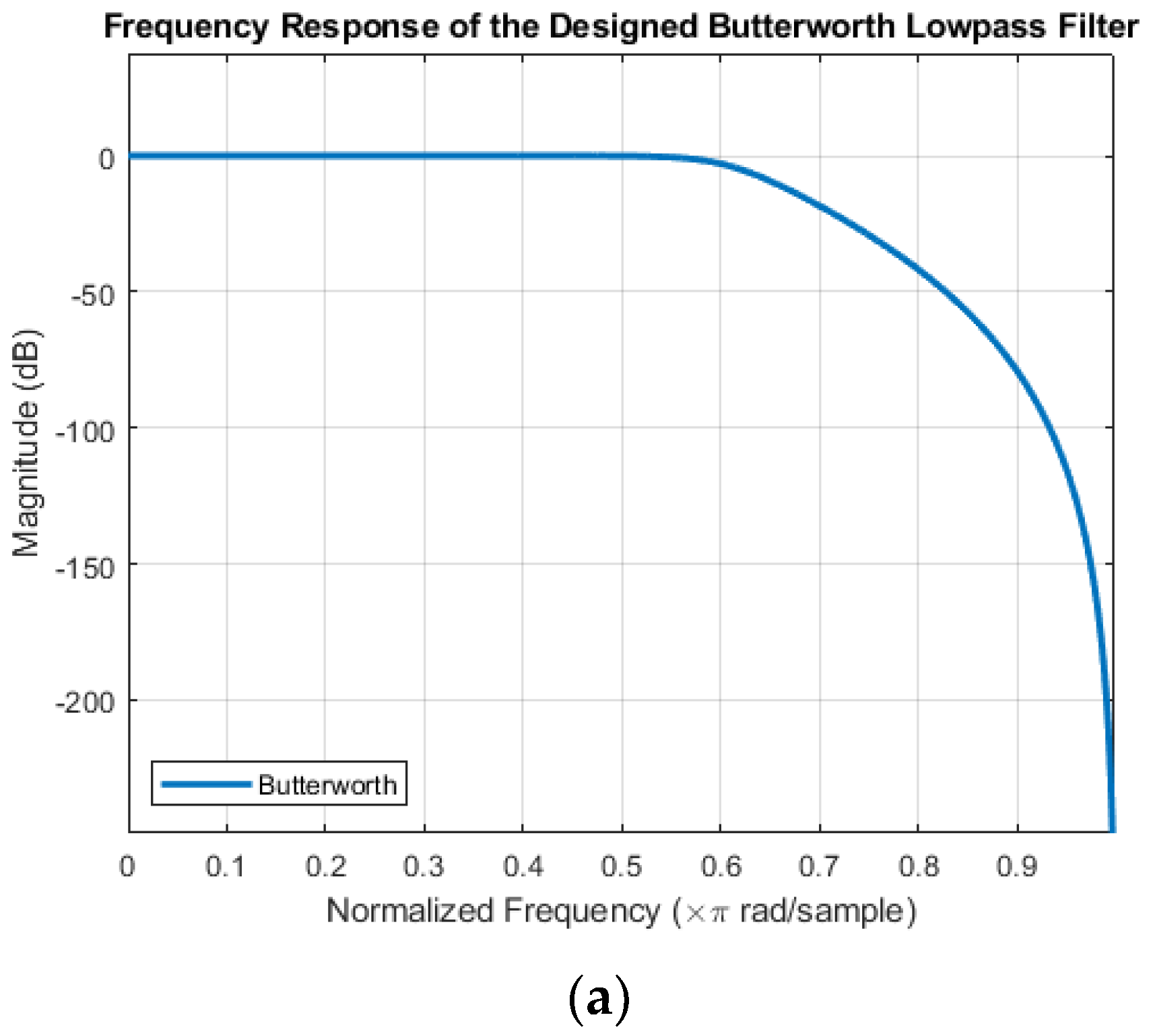
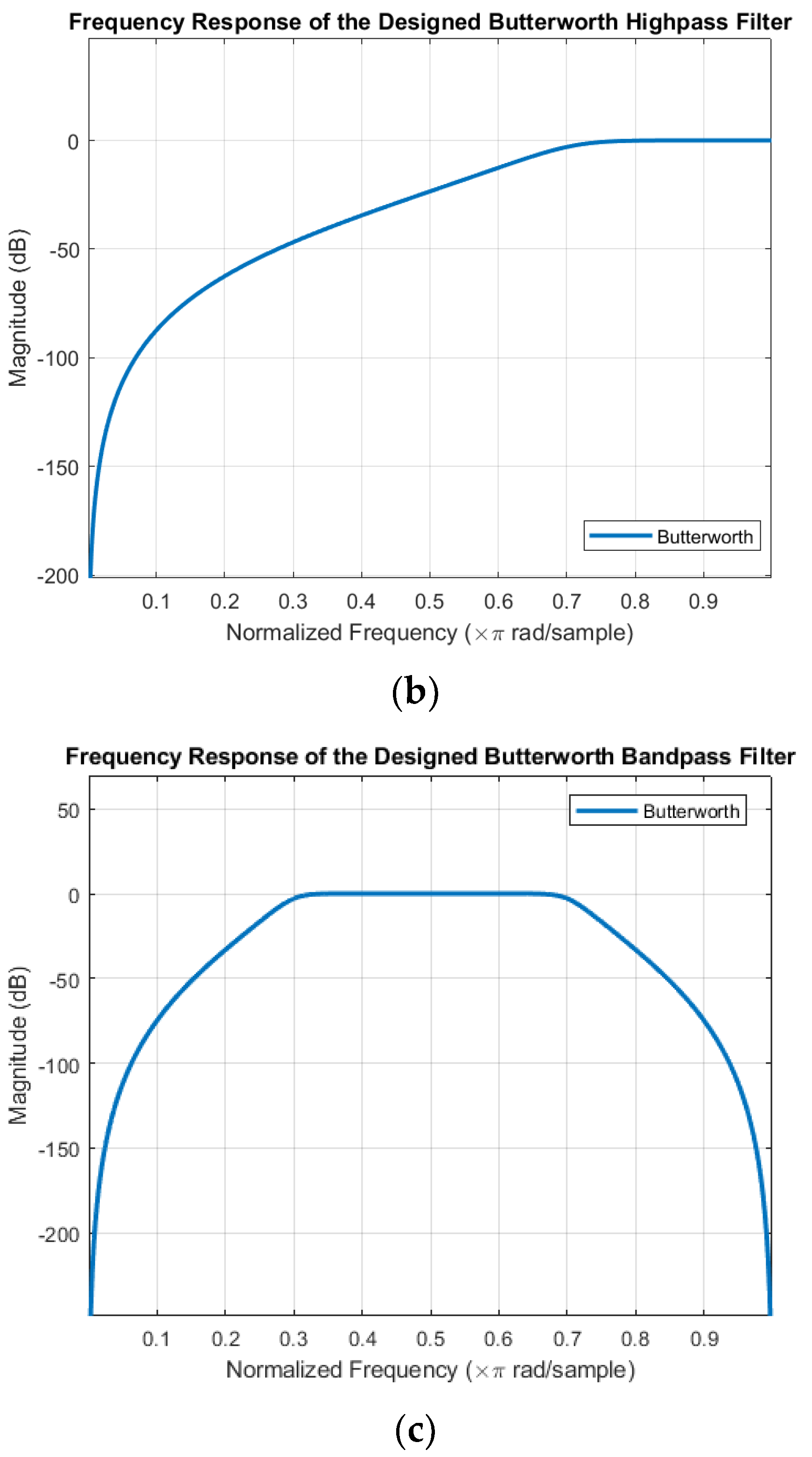
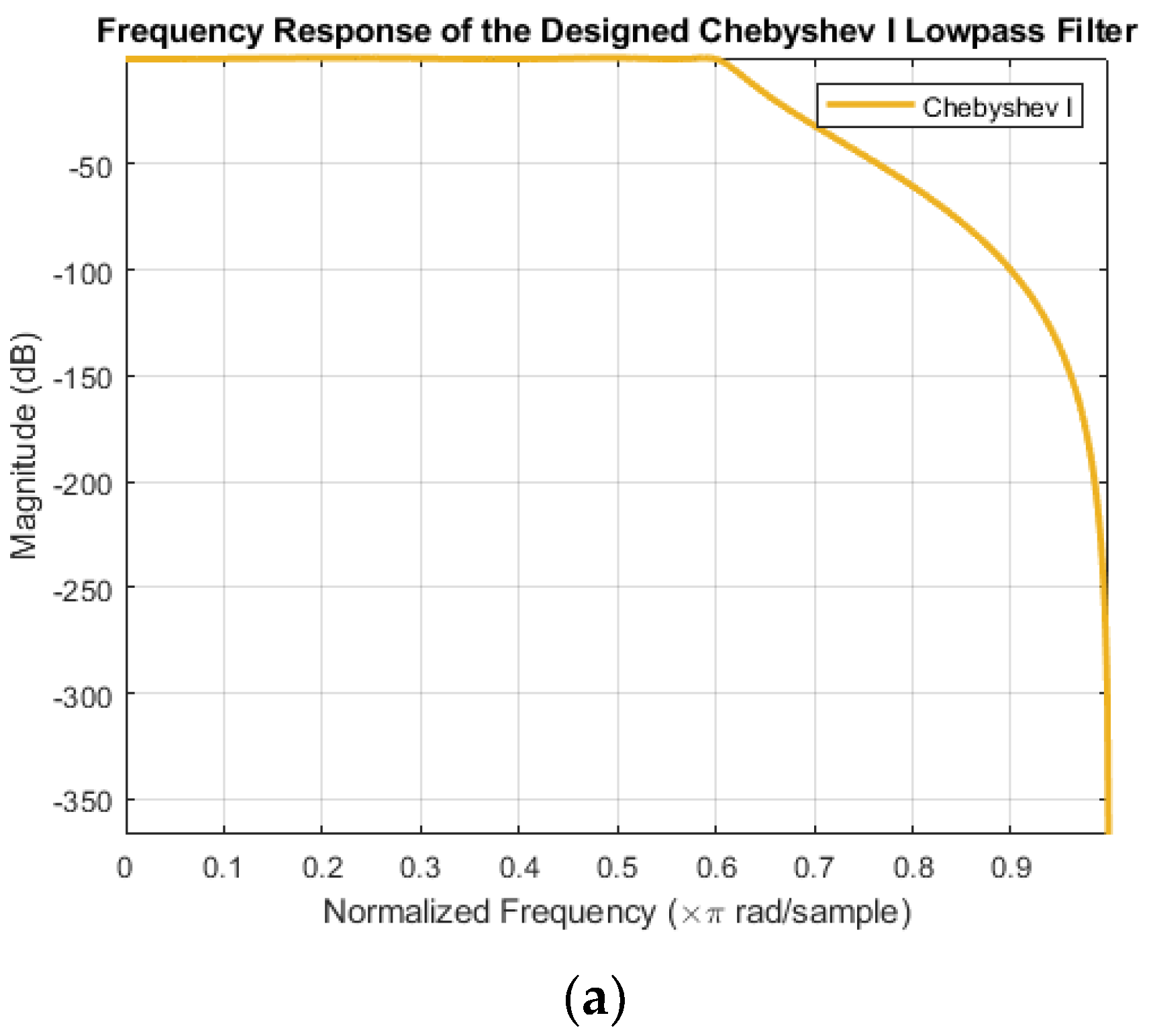
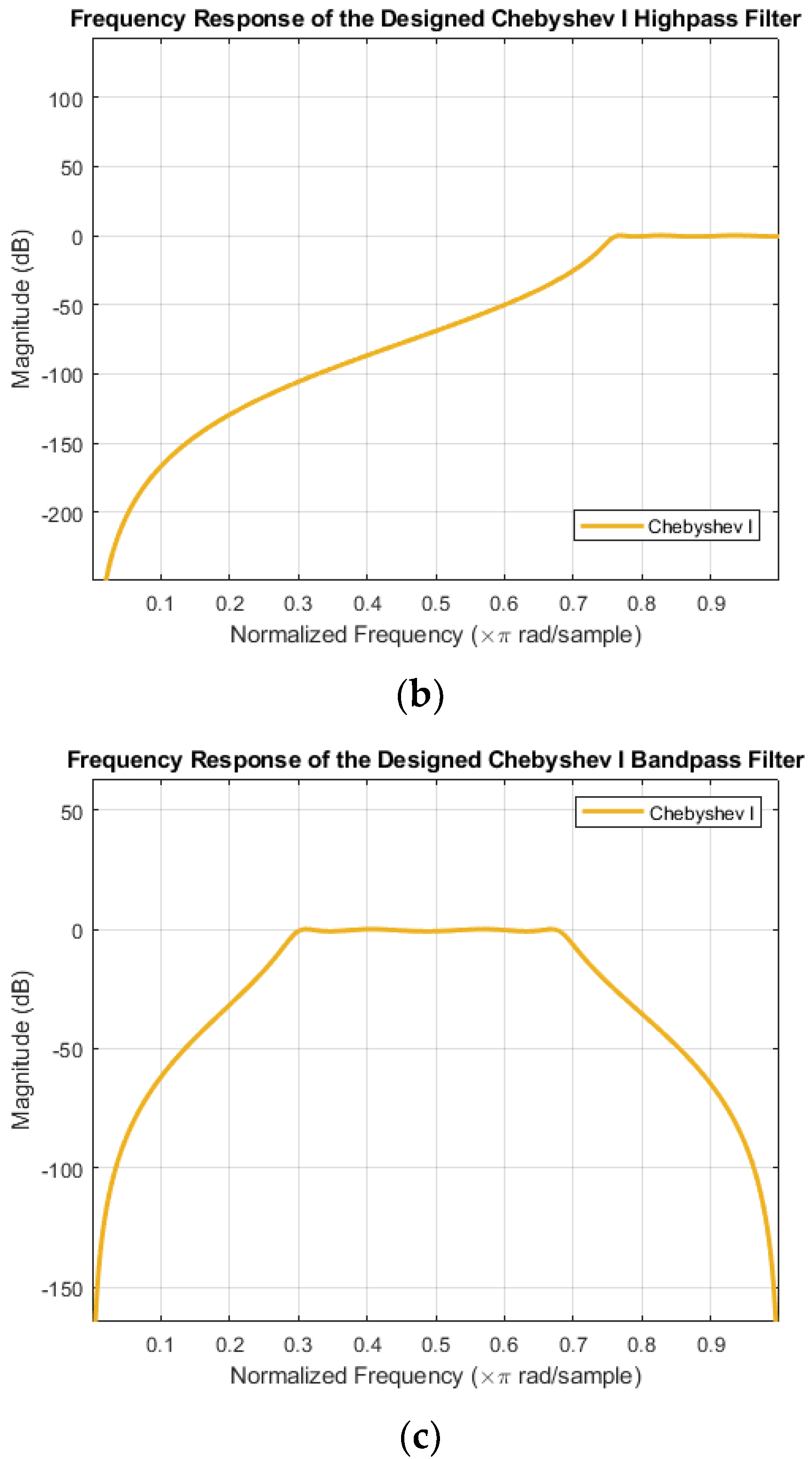
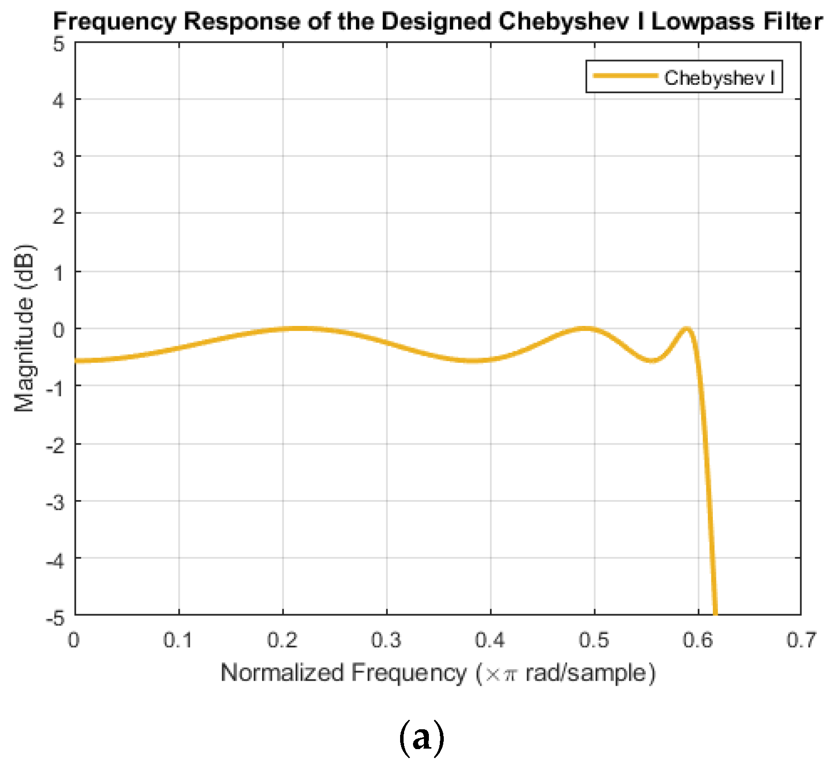
Figure 3 and Figure 4 are three filter types designed based on Butterworth and Chebyshev Type I characteristics. One has no passband oscillation, and the other has passband os-cillation. However, with the filter, practical considerations will cause the passband to os-cillate between 0 and 1 (dB) and speed up the roll-off. Figure 5 shows Chebyshev Type I Filter Passband Ripple Enlarged View.
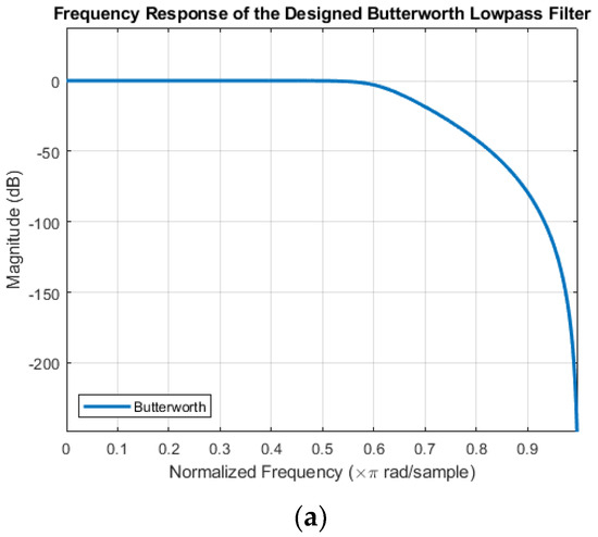
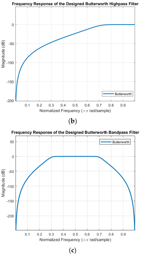
Figure 3.
(a) Design of Butterworth low–pass filter. (b) Design of Butterworth high–pass filter. (c) Design of Butterworth band–pass filter.

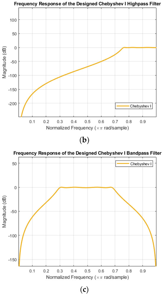
Figure 4.
(a) Design of Chebyshev Type I low–pass filter. (b) Design of Chebyshev Type I high–pass filter. (c) Design of Chebyshev Type I band–pass filter.
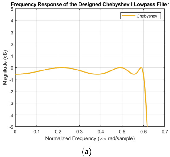

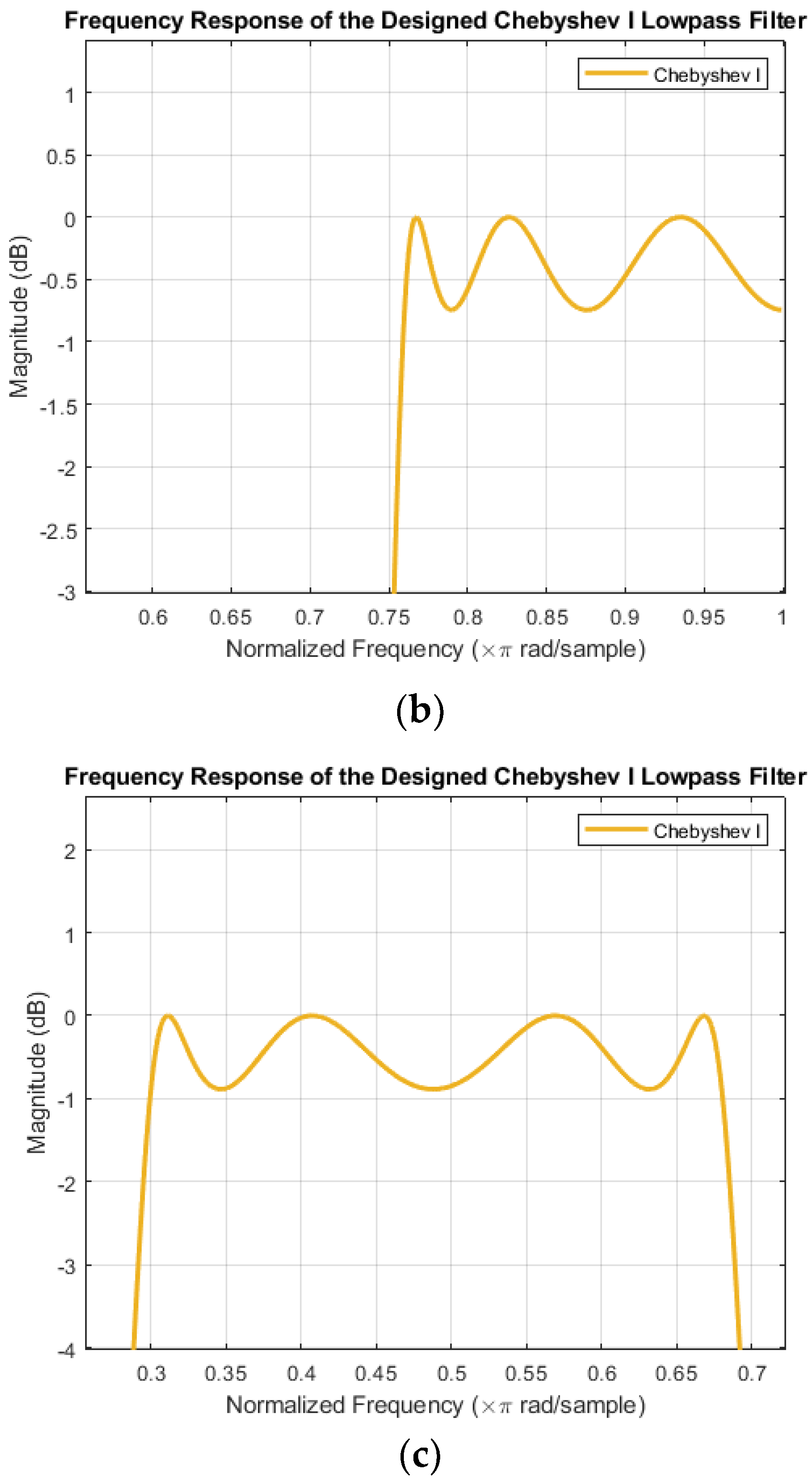
Figure 5.
(a) Chebyshev Type I low–pass filter passband ripple enlarged view. (b) Chebyshev Type I high–pass filter passband ripple enlarged view. (c) Chebyshev Type I band–pass filter passband ripple enlarged view.
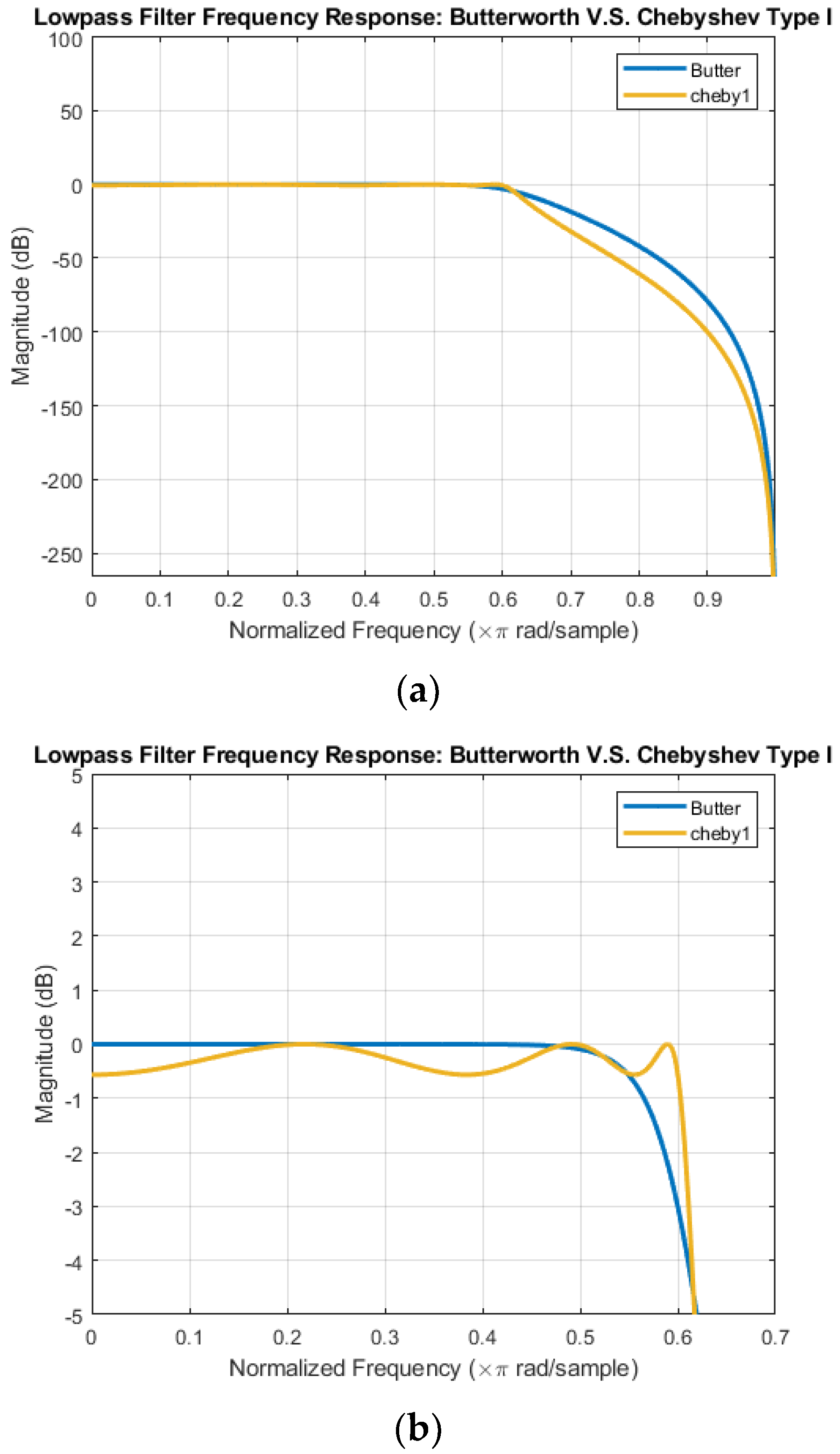
The difference in the responses can be seen in Figure 6; although the low-pass filters designed using the same design parameters look similar in the filter transition bandwidth, the roll-off decreases the speed. The descent speed of Upper Chebyshev I is slightly faster than Butterworth’s. To make the roll-off speed faster, one can also re-adjust the parameters of the particle swarm to achieve a faster roll-off, but this will cause the problem of large passband oscillation. In practical applications, most people still hope to have a smooth and stable passband, especially when processing audio. They hope the passband will be stable to maintain signal stability and complete noise filtering.
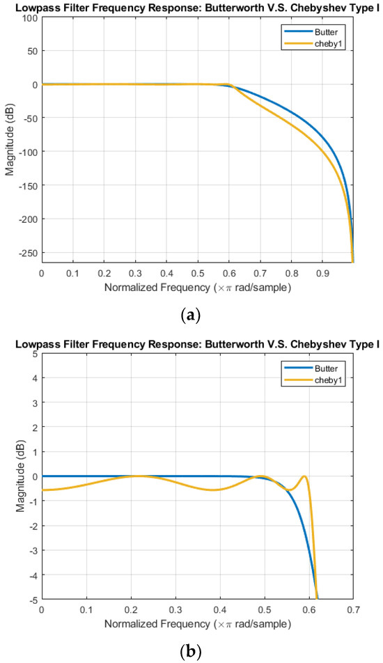
Figure 6.
(a) Low–pass filter comparison chart. (b) Low–pass filter comparison chart passband ripple enlarged view.
Table 2 randomly generates a section of white noise and filters it through the designed filter. The signal-to-noise ratio is calculated before and after filtering to ensure the designed filter can effectively filter.
Table 2.
SNR comparison.
4. Discussion
This study has greatly improved the process of the multi-objective particle swarm optimization algorithm. Compared with the particle swarm optimization method proposed by Haruna Aimi and other scholars [11] and Kenzo Yamamoto and other scholars [11], by calculating the MMSE, ME, and SD, this study optimized the following two parts.
- Optimization of frequency response
The particle swarm optimization algorithm, combined with Pareto efficiency, can find the best balance between multiple objectives, such as between the frequency response of the passband and stopband, which can help design a design that satisfies the frequency within the passband requirements and can effectively suppress the stopband frequency filter.
- 2.
- Optimization of selectivity and bandwidth
The selectivity (the ability to distinguish the passband and stopband) and bandwidth of the filter are essential considerations in design. The particle swarm optimization algorithm combined with Pareto efficiency can improve the selectivity while appropriately controlling the bandwidth to achieve the best compromise between these two aspects.
Comparison with Related Literature
Table 3.
Design parameters used in the literature.
and are the numerator and denominator of the filter transfer function. is the expected group delay. is the passband frequency edge frequency. is the stopband edge frequency. is the maximum value of the pole radius. is the number of particles. is the maximum number of iterations.
Using the same design parameters as in the literature (as shown in Table 3) to perform filter design, in Table 4 and Table 5, our approach demonstrates superior or comparable performance in filter design, with lower error rates and more consistent results. This validates the effectiveness of our PSO-based method for multi-objective optimization in IIR filter design, outperforming the methods proposed by Haruna Aimi et al. [11] and Yamamoto et al. [12].
Table 4.
Comparison of results to those of Haruna Aimi et al.
Table 5.
Comparison of results to those of Yamamoto et al.
In summary, combined with Pareto efficiency, the particle swarm optimization algorithm can more effectively identify the optimal balance point between multiple objectives and provide a set of Pareto optimal solutions, which helps solve multi-objective optimization problems. It is beneficial, and this method is suitable for continuous problems and can effectively solve discrete problems. It does not require making assumptions about the specific form of the problem (such as the linearity or nonlinearity of the objective function), making it very adaptable and powerful.
5. Conclusions
This study realizes the “multi-objective particle swarm optimization algorithm applied to the design of infinite impulse response filter” using the particle swarm algorithm combined with Pareto efficiency. This method takes advantage of the global search capability. The multi-objective optimization concept of the Pareto frontier effectively solves the multi-objective conflict problems existing in traditional infinite impulse response filter design, especially the balance between passband and stopband performance filter orders and qualitative questions. Under the same conditions as other references, this research method can reach 1.83 and 2.83 in MMSE, 2.34 and 3.34 in ME, and 0.03 and 2.72 in SD. It has been proven that through the optimization method proposed in this study, a better balance can be achieved between multiple objectives, significantly minimizing passband oscillation and maximizing stopband suppression. Thus, the cutoff frequency can be guaranteed, and the filter order, passband, and stopband performance can meet predetermined specifications. These are essential factors to consider in filter design.
Author Contributions
Conceptualization, Q.-Y.Z.; Software, W.-R.Y.; Formal analysis, W.-H.L.; Investigation, Y.-C.H.; Resources, W.-H.L., Y.-C.H. and S.-M.W.; Writing—original draft, Q.-Y.Z.; Writing—review & editing, T.-J.S.; Supervision, T.-J.S.; Project administration, Q.-Y.Z. and S.-M.W. All authors have read and agreed to the published version of the manuscript.
Funding
This research is supported financially in part by the National Science and Technology Council, ROC (No. 113-2221-E-230-004-) and ICP DAS Co., Ltd.
Data Availability Statement
The original contributions presented in the study are included in the article, further inquiries can be directed to the corresponding author.
Conflicts of Interest
The authors declare no conflict of interest.
References
- Chauhan, R.S.; Mehra, R.; Shallu. ASIC design of IIR butterworth digital filter for electrocardiogram. In Proceedings of the 2017 8th International Conference on Computing, Communication and Networking Technologies (ICCCNT), Delhi, India, 3–5 July 2017; pp. 1–6. [Google Scholar]
- Podder, P.; Hasan, M.M.; Islam, M.R.; Sayeed, M. Design and implementation of Butterworth, Chebyshev-I and elliptic filter for speech signal analysis. arXiv 2020, arXiv:2002.03130. [Google Scholar] [CrossRef]
- Ardakani, A.; Leduc-Primeau, F.; Gross, W.J. Hardware implementation of FIR/IIR digital filters using integral stochastic computation. In Proceedings of the 2016 IEEE International Conference on Acoustics, Speech and Signal Processing (ICASSP), Shanghai, China, 20–25 March 2016; pp. 6540–6544. [Google Scholar]
- Getu, B.N. Digital IIR Filter Design using Bilinear Transformation in MATLAB. In Proceedings of the 2020 International Conference on Communications, Computing, Cybersecurity, and Informatics (CCCI), Sharjah, United Arab Emirates, 3–5 November 2020; pp. 1–6. [Google Scholar]
- Agrawal, N.; Kumar, A.; Bajaj, V.; Singh, G. Design of digital IIR filter: A research survey. Appl. Acoust. 2021, 172, 107669. [Google Scholar] [CrossRef]
- Loubna, K.; Bachir, B.; Izeddine, Z. Optimal digital IIR filter design using ant colony optimization. In Proceedings of the 2018 4th International Conference on Optimization and Applications (ICOA), Mohammedia, Morocco, 26–27 April 2018; pp. 1–5. [Google Scholar]
- Agrawal, N.; Kumar, A.; Bajaj, V. A new method for designing of stable digital IIR filter using hybrid method. Circuits Syst. Signal Process. 2019, 38, 2187–2226. [Google Scholar] [CrossRef]
- Matei, R. Analytic design of directional and square-shaped 2D IIR filters based on digital prototypes. Multidimens. Syst. Signal Process. 2019, 30, 2021–2043. [Google Scholar] [CrossRef]
- Agrawal, N.; Kumar, A.; Bajaj, V. Optimized design of digital IIR filter using artificial bee colony algorithm. In Proceedings of the 2015 International Conference on Signal Processing, Computing and Control (ISPCC), Waknaghat, India, 24–26 September 2015; pp. 316–321. [Google Scholar]
- Sharaf, A.M.; El-Gammal, A.A.A. A novel discrete multi-objective Particle Swarm Optimization (MOPSO) of optimal shunt power filter. In Proceedings of the 2009 IEEE/PES Power Systems Conference and Exposition, Seattle, WA, USA, 15–18 March 2009; pp. 1–7. [Google Scholar]
- Aimi, H.; Suyama, K. Design of IIR filters by determining particle reallocation space using multi-swarm PSO. In Proceedings of the 2015 15th International Symposium on Communications and Information Technologies (ISCIT), Nara, Japan, 7–9 October 2015; pp. 29–32. [Google Scholar]
- Yamamoto, K.; Suyama, K. Active enumeration of local minima for IIR filter design using PSO. In Proceedings of the 2017 Asia-Pacific Signal and Information Processing Association Annual Summit and Conference (APSIPA ASC), Kuala Lumpur, Malaysia, 12–15 December 2017; pp. 910–917. [Google Scholar]
- Dhanarasi, G.; Kumar, P.S.; Krishna, B.T. Design of Infinite Impulse Response Filter Using Particle Swarm Optimization and its Invariants. In Proceedings of the 2022 International Conference on Smart and Sustainable Technologies in Energy and Power Sectors (SSTEPS), Mahendragarh, India, 7–11 November 2022; pp. 306–310. [Google Scholar]
- Takase, Y.; Suyama, K. A Diversification Strategy for IIR Filter Design Using PSO. In Proceedings of the 2018 Asia-Pacific Signal and Information Processing Association Annual Summit and Conference (APSIPA ASC), Honolulu, HI, USA, 12–15 November 2018; pp. 1365–1369. [Google Scholar]
- Antoniou, A. Digital Filters: Analysis, Design and Applications, 2nd ed.; McGraw-Hill Education (ISE Editions): New York, NY, USA, 1993. [Google Scholar]
- Wang, D.; Tan, D.; Liu, L. Particle swarm optimization algorithm: An overview. Soft Comput. 2018, 22, 387–408. [Google Scholar] [CrossRef]
- Federico, M.; Walczak, B. Particle swarm optimization (PSO). A Tutor. Chemom. Intell. Lab. Syst. 2015, 149, 153–165. [Google Scholar]
- Gad, A.G. Particle swarm optimization algorithm and its applications: A systematic review. Arch. Comput. Methods Eng. 2022, 29, 2531–2561. [Google Scholar] [CrossRef]
- Saptarshi, S.; Basak, S.; Peters, R.A. Particle Swarm Optimization: A survey of historical and recent developments with hybridization perspectives. Mach. Learn. Knowl. Extr. 2018, 1, 157–191. [Google Scholar] [CrossRef]
- Cheng, R.; Jin, Y. A social learning particle swarm optimization algorithm for scalable optimization. Inf. Sci. 2015, 291, 43–60. [Google Scholar] [CrossRef]
- Ganjehkaviri, A.; Jaafar, M.M.; Hosseini, S.E.; Barzegaravval, H. Genetic algorithm for optimization of energy systems: Solution uniqueness, accuracy, Pareto convergence and dimension reduction. Energy 2017, 119, 167–177. [Google Scholar] [CrossRef]
- Figueiredo, E.M.; Ludermir, T.B.; Bastos-Filho, C.J. Many objective particle swarm optimization. Inf. Sci. 2016, 374, 115–134. [Google Scholar] [CrossRef]

Disclaimer/Publisher’s Note: The statements, opinions and data contained in all publications are solely those of the individual author(s) and contributor(s) and not of MDPI and/or the editor(s). MDPI and/or the editor(s) disclaim responsibility for any injury to people or property resulting from any ideas, methods, instructions or products referred to in the content. |
© 2024 by the authors. Licensee MDPI, Basel, Switzerland. This article is an open access article distributed under the terms and conditions of the Creative Commons Attribution (CC BY) license (https://creativecommons.org/licenses/by/4.0/).