Abstract
In brain–computer interface motor imagery (BCI-MI) systems, convolutional neural networks (CNNs) have traditionally dominated as the deep learning method of choice, demonstrating significant advancements in state-of-the-art studies. Recently, Transformer models with attention mechanisms have emerged as a sophisticated technique, enhancing the capture of long-term dependencies and intricate feature relationships in BCI-MI. This research investigates the performance of EEG-TCNet and EEG-Conformer models, which are trained and validated using various hyperparameters and bandpass filters during preprocessing to assess improvements in model accuracy. Additionally, this study introduces EEG-TCNTransformer, a novel model that integrates the convolutional architecture of EEG-TCNet with a series of self-attention blocks employing a multi-head structure. EEG-TCNTransformer achieves an accuracy of 83.41% without the application of bandpass filtering.
1. Introduction
Artificial intelligence (AI) is versatile and supports people in various areas, such as intelligent medicine, transportation, education, and entertainment. Brain–control interface (BCI) is a research field in AI that learns and extracts information in human brain waves to control assistive devices such as prosthetic hands [1], intelligent wheelchairs [2], and exoskeletons [3]. In 2013, the Centers for Disease Control and Prevention estimated that about 5.4 million people, which accounted for 1.7% of the United States population, had been living with paralysis [4]. Regarding the methods for collecting brain waves, BCI can be categorised into invasive, partially invasive, and non-invasive. Electrode devices are implanted directly into human skulls for invasive methods. However, the risk and potential complications after surgery have restricted patients to invasive methods. Non-invasive methods place electrodes on the scalp’s surface to record data. There are many non-invasive modalities, such as electroencephalography (EEG) [5], positron emission tomography (PET) [6], magnetoencephalography (MEG) [7], functional near-infrared spectroscopy (fNIRS) [8], and magnetic resonance imaging (fMRI) [9].
Convolutional neural network methods have contributed to most of the significantly advanced studies in brain–control interfaces by effectively extracting spatial and temporal features from EEG signals. However, the emergence of Transformer methods, which have advanced techniques with powerful self-attention mechanisms, promises to enhance the modelling of long-term dependencies and feature relationships. This study explores the integration of CNN and Transformer techniques, aiming to leverage their combined strengths for improved accuracy and efficiency in motor imagery BCI applications. By extensively evaluating the EEG-TCNet and EEG-Conformer models, including their architecture, hyperparameters, and the impact of bandpass filtering, this research seeks to identify the most effective strategies for enhancing overall performance. Additionally, this study introduces EEG-TCNTransformer, a novel BCI-MI model that incorporates TCN and self-attention and achieves an accuracy of 83.41% without a bandpass filter. The source code of EEG-TCNTransformer isavailable on GitHub, accessed on 17 September 2024.
2. Background
Traditional machine learning methods require handcrafted feature extractors and a classification network. In terms of extracting the spatial features, a common spatial pattern (CSP) [10] and an extended version of CSP, which is a filter bank CSP (FBCSP) [11], are the most common methods. Moreover, short-time Fourier transform (STFT) [12] and continuous wavelet transform (CWT) [13] are used to extract the time–frequency features. Additionally, the feature extractors must be combined with classification, such as support vector machine (SVM) [14], Bayesian classifier [11], and linear discriminant analysis (LDA) [15], to classify the target tasks. However, EEG signals are non-stationary and have a low signal-to-noise ratio, so deep learning methods are researched to improve the weaknesses of traditional machine learning methods.
Regarding traditional deep learning methods, convolutional neural network (CNN) methods are the most common methods that achieve various state-of-the-art studies. Lawhern proposed EEGNet [16], which is applied to multiple BCI paradigms, including movement-related cortical potentials (MRCPs), error-related negativity responses (ERNs), sensory-motor rhythms (SMRs), and P300 visual-evoked potentials. ShallowNet, proposed by Schirrmeister (2017) [17], measures the performance of different deep levels in convolution networks, from 5 convolution layers to 31 convolution layer residual networks, using ResNet architecture. EEG-TCNet [18] incorporates convolution layers in EEGNet and temporal convolutional networks (TCNs) [19], which can exponentially increase the receptive field size by using dilated causal convolution [20,21]. Moreover, recurrent neural networks (RNNs), gated recurrent unit (GRU), and long short-term memory (LSTM) are combined with CNN methods to learn long sequence data [22].
The transformer method is an advanced method that allows the learning of features in parallel and improves the learning of long sequence dependency [23]. Because of the structure of multi-head attention, the transformer method can efficiently capture the relationships in features through attention mechanisms. Liu proposed a Transformer-based one-dimensional convolutional neural network model (CNN-Transformer), which uses 1D-CNN to extract low-level time–frequency features and a transformer module to extract higher-level features [24]. Hybrid CNN-Transformer [25] was proposed as a complex architecture with spatial Transformer and spectral Transformer to encode raw EEG signals to an attention map, and then utilise CNN to explore the local features and temporal Transformer to perceive global temporal features. EEG-Conformer [26], proposed by Song, is a lightweight model with a shallow convolution to extract temporal and spatial features and self-attention mechanisms to learn the relationships in the time domain.
This study aims to research the contributions of different hyperparameters and different bandpass filter parameters to the CNN method and the Transformer method in MI-BCI. EEG-TCNet and EEG-Conformer were selected for this study. Therefore, there are two sub-projects, as follows:
- First sub-project: EEG-TCNet and EEG-Conformer are trained and validated with different hyperparameters (i.e., filters, kernel sizes).
- Second sub-project: EEG signals are preprocessed with a bandpass filter, then input in training and testing EEG-TCNet and EEG-Conformer.
In this research, a new model is introduced, EEG-TCNTransformer, inspired by EEG-TCNet and EEG-Conformer. EEG-TCNTransformer has the advantage of learning low-level temporal features and spatial features by the novel convolution architecture from EEG-TCNet and extracting the global temporal correlation from the self-attention mechanism. Moreover, EEG-TCNTransformer uses raw EEG data, so the bandpass filter is omitted.
3. Methods
3.1. Dataset
The data studied in this project are from the BCI Competition in 2008 [27]. Data Group 2A, accessed on 17 September 2024, is a set of experimental data on motor imagery for electric wheelchair control. It includes four motor tasks: move the left hand, move the right hand, move both feet, and move the tongue, which represent turn left, turn right, move forward, and move backward, respectively. This dataset includes 22 EEG channels and 3 EOG channels, collected from 9 participants over 2 sessions on 2 different days. Each session consists of 6 runs with 48 trials each. The data from each session are stored in one MATLAB file.
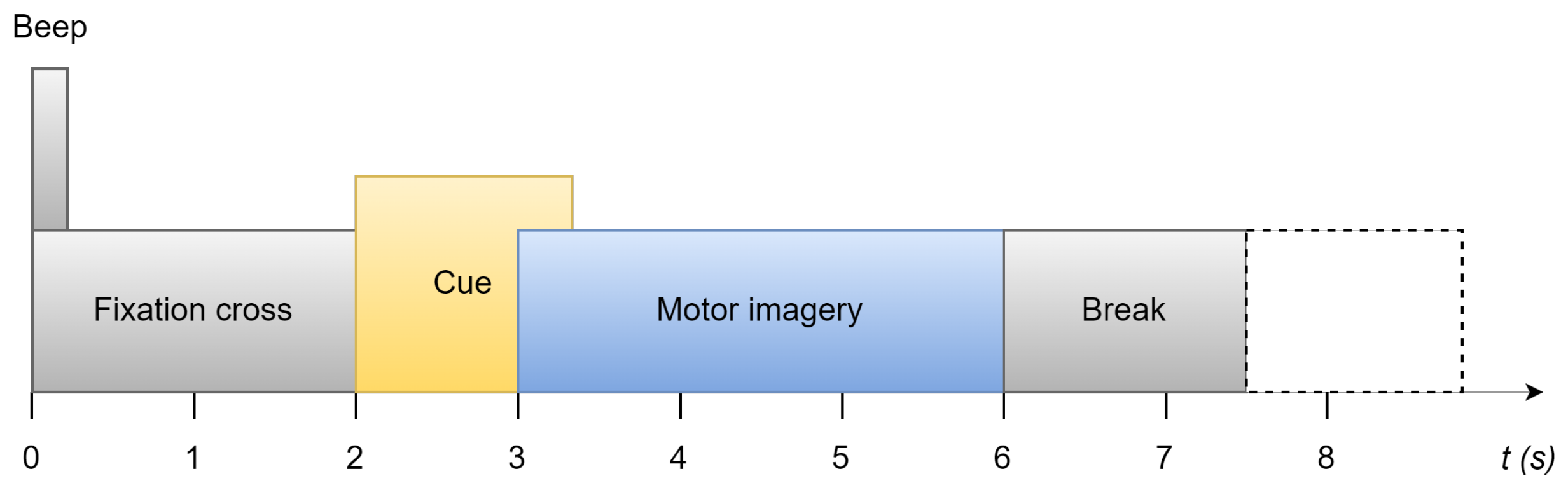
In Figure 1, each trial is between 7.5 s and 8.5 s. It starts with a prompt beep and a cross displayed on the screen. Two seconds later, the cue of this trial displays on the screen in the form of an arrow. The four directions it points to represent moving forward, moving backward, turning left, and turning right. This instruction stays on the screen for 1.25 s. The participant is required to perform motor imagery for the next 3 s. At the end of the trial, there is a 1.5 s short break before the next trial, which could be increased randomly to 2.5 s to avoid adaption.
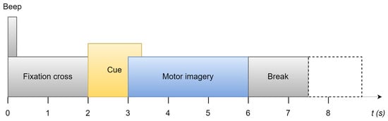
Figure 1.
Time scheme of data record [27].
At the beginning of the data collection, EOG data for each subject were also recorded for the elimination of interference information. These EOG data are removed from this study.
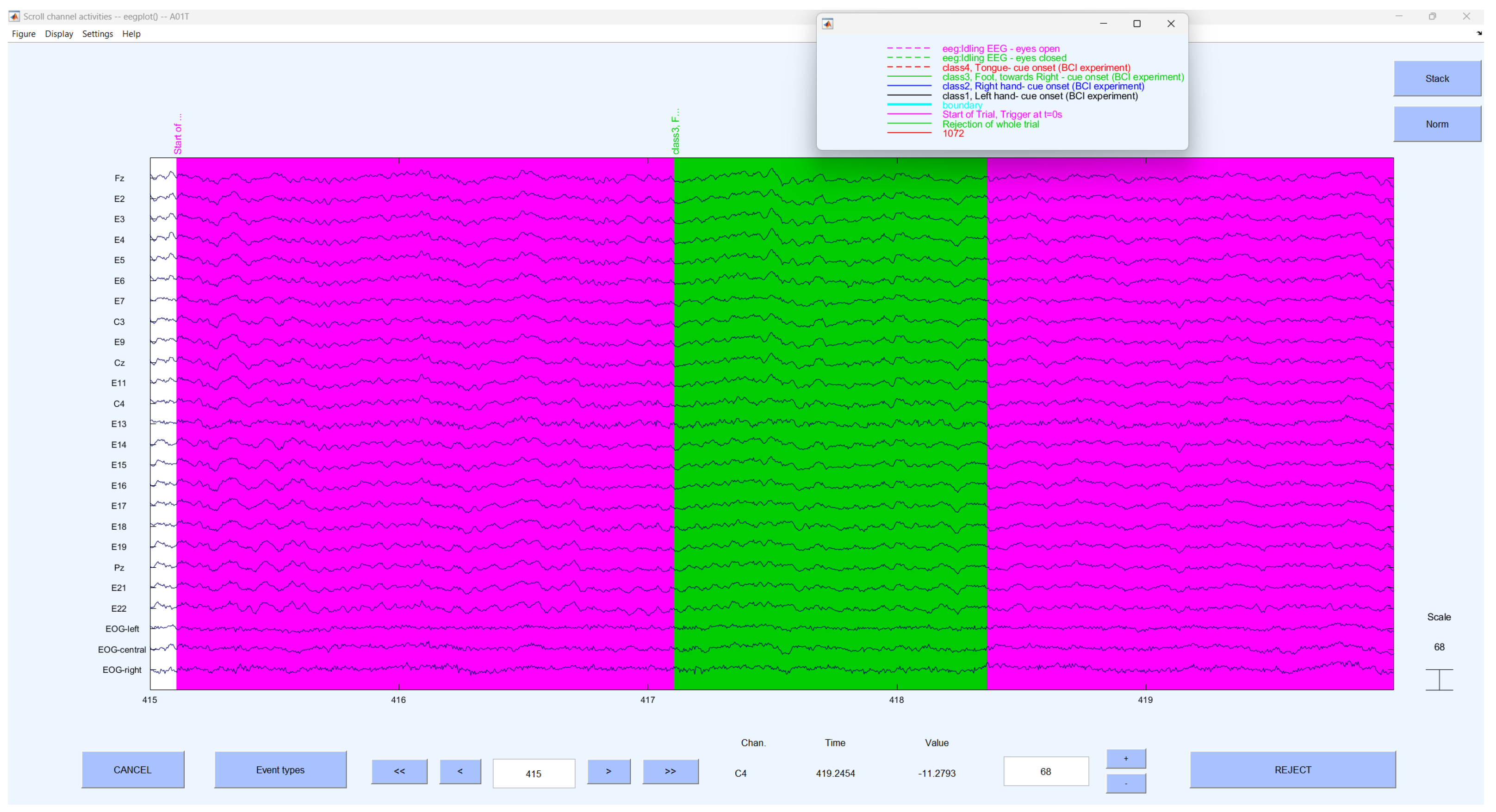
In this study, EEG-LAB is used as the primary tool for data visualisation. EEG-LAB is an add-on for MATLAB that provides various features for analysing electrophysiological data, including processing of EEG, visualisation, and integration of algorithms. Figure 2 shows the visualisation of the EGG signals in EEG-LAB.

Figure 2.
EEG signals visualised in EEG-LAB.
3.2. Preprocessing
Data preprocessing was conducted to ensure the best and most relevant data for training the models, employing multiple techniques.
The three extra EOG channels measure eye movements and are easily influenced by non-study-induced factors such as attention levels and blinks. Therefore, these channels were excluded from training to avoid introducing noise and confounding variables.
During motor imagery, there is usually a change in neural oscillations indicating Event-Related Desynchronisation (ERD) and Event-Related Synchronisation (ERS), which are mostly observed in the alpha (8–13 Hz) and beta frequency bands (18–24 Hz) [28]. These provide good features for model training. Signal filtration was employed to increase the signal-to-noise ratio. The sharp transition band between the pass and stop bands, as well as the low ripple in the pass band, made the Chebyshev type 2 bandpass filter (Figure 3) the filter of choice. The effectiveness of this filter is primarily determined by the order of the filter N and, to a lesser extent, the stop-band attenuation requirement . The amplitude response is given as
where
| is parameter related to the ripples in the stop-band; | |
| is the nth-order Chebyshev polynomial; | |
| is the stop-band edge frequency; and | |
| f | is the frequency variable. |
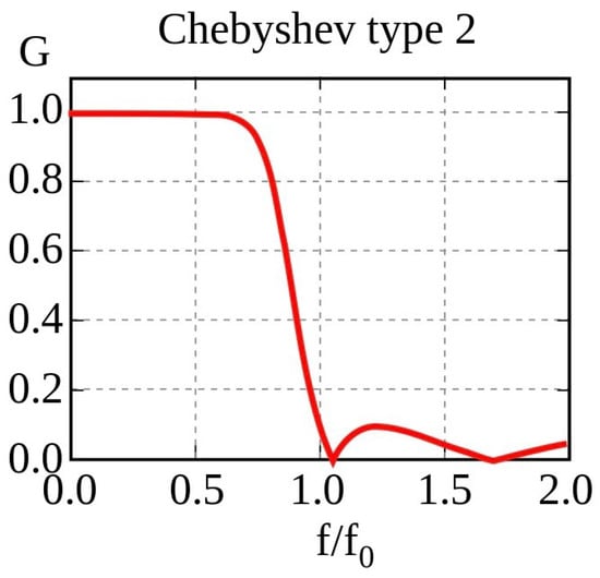
Figure 3.
Transfer function of the Chebyshev filter (type 2) [29].
The ripple factor is related to the stop-band attenuation by
These two hyperparameters, N and , were included in the hyperparameter optimisation process.
In addition, z-score normalisation is applied to the signals to ensure that all channels are on the same scale, increasing comparability and handling variability in the dataset. The z-score normalisation is defined as
where
| z | is the standardised value; |
| x | is the original value; |
| is the mean of the distribution; and | |
| is the standard deviation of the distribution |
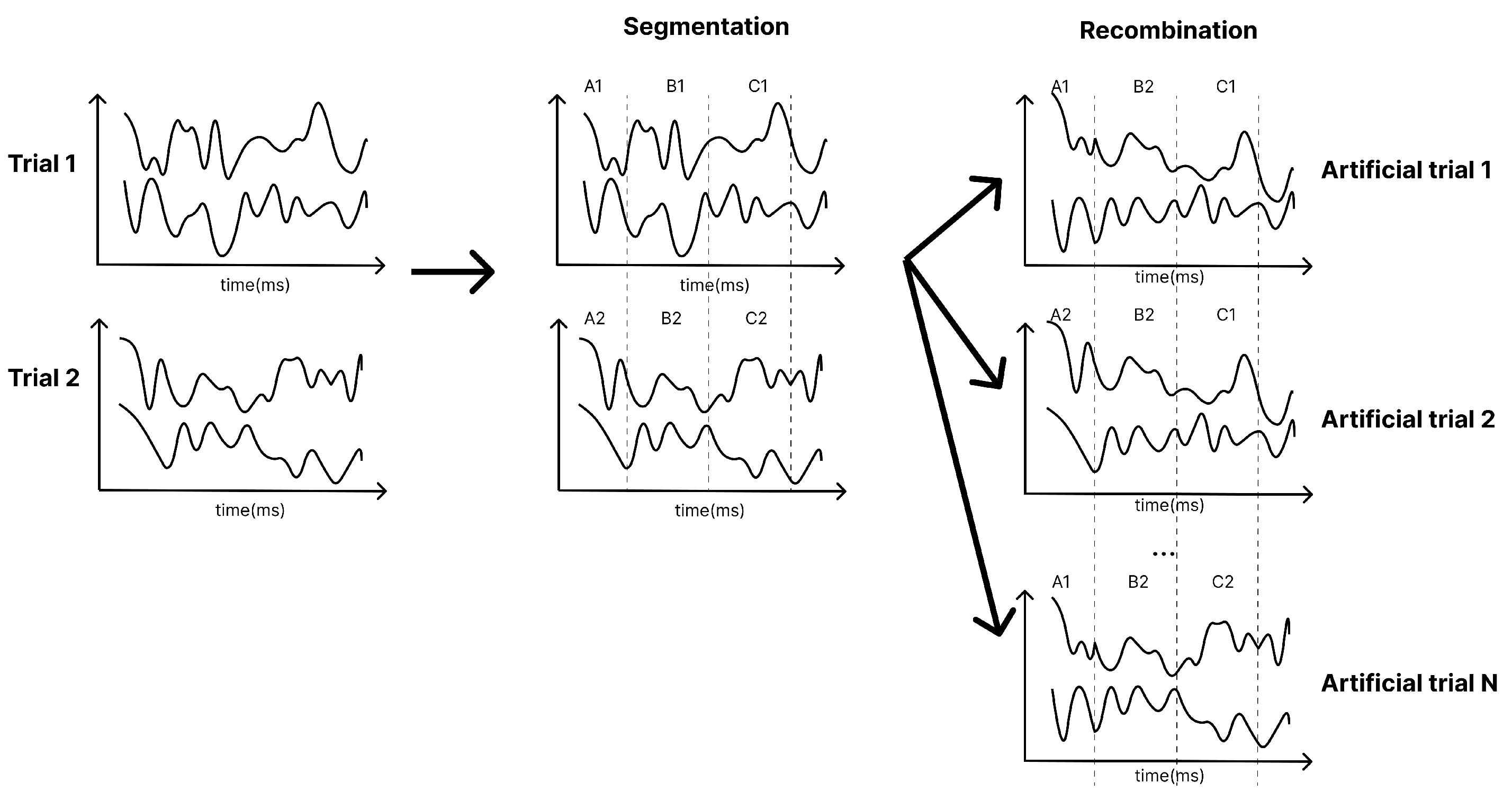
Furthermore, due to the limited size of the training dataset, data augmentation was applied by segmenting and recombining signals in the time domain [30]. As illustrated in Figure 4, each training trial is divided into multiple non-overlapping segments. A large amount of new data are generated by randomly concatenating segments from different trials of the same class. This technique was specifically applied to the Conformer model. Further research is needed to analyse the impact of data augmentation across a broader range of models.
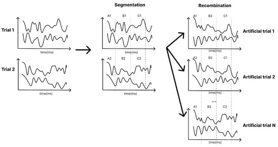
Figure 4.
Segmentation and reconstruction (R&S) augmentation in time domain [30]. Trial 1 cut into A1, B1, and C1 and trial 2 cut into A2, B2, and C2. In the recombination stage, each output trial randomly combines 3 segments of A1, B1, C1, A2, B2, and C2. Artificial trial 1 combines A1, B2, and C1.
3.3. EEG-TCNet
The first model in this study is EEG-TCNet, which is incorporated from the EEGNet and TCN modules. The EEGNet module in EEG-TCNet is slightly modified, with 2D temporal convolution at the beginning to extract the frequency filters, followed by a depthwise convolution to extract frequency-specific spatial filters. The third part of the EEGNet module is a separable convolution extract temporal summary for each feature map from depthwise convolution and mixes the feature maps before going into the TCN module.
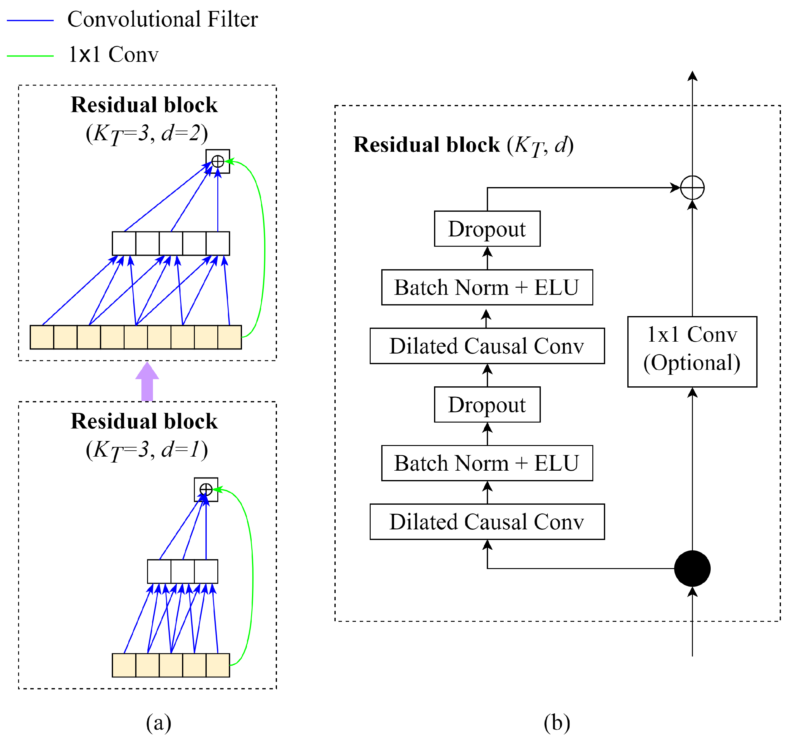
Regarding the TCN module, based on the idea of the temporal convolutional network (TCN), the TCN module in EEG-TCNet could be described as follows (Figure 5):
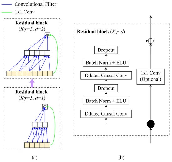
Figure 5.
Architecture elements in a TCN. (a) Stacking of two residual blocks with dilated causal convolution with dilation factors d = 1, 2 and kernel size k = 3. (b) Detailed layers in TCN residual block [19].
- (a)
- Causal Convolutions: TCN aims to produce the output of the same size as the input, so TCN uses a 1D fully convolutional network with each hidden layer having the same size as the input layer. To keep the length of subsequent layers equal to the previous ones, zero padding of length (kernel size: 1) is applied. Moreover, to prevent information leakage from a feature to the past in training, only the inputs from time t and earlier determine the output at time t.
- (b)
- Dilated Convolutions: The major disadvantage of regular causal convolutions is that the network must be extremely deep or have large filters to obtain a large receptive field size. A sequence of dilated convolutions could increase the receptive field exponentially by increasing dilation factors d.
- (c)
- Residual Blocks: In EEG-TCNet, the weight normalisation in the original TCN is replaced by batch normalisation. The residual blocks have a stack of two layers of dilated convolution, batch normalisation with ELU, and dropout. The skip connection 1 × 1 convolution is applied from the input to the output feature map to ensure the same shape of input and output tensors.
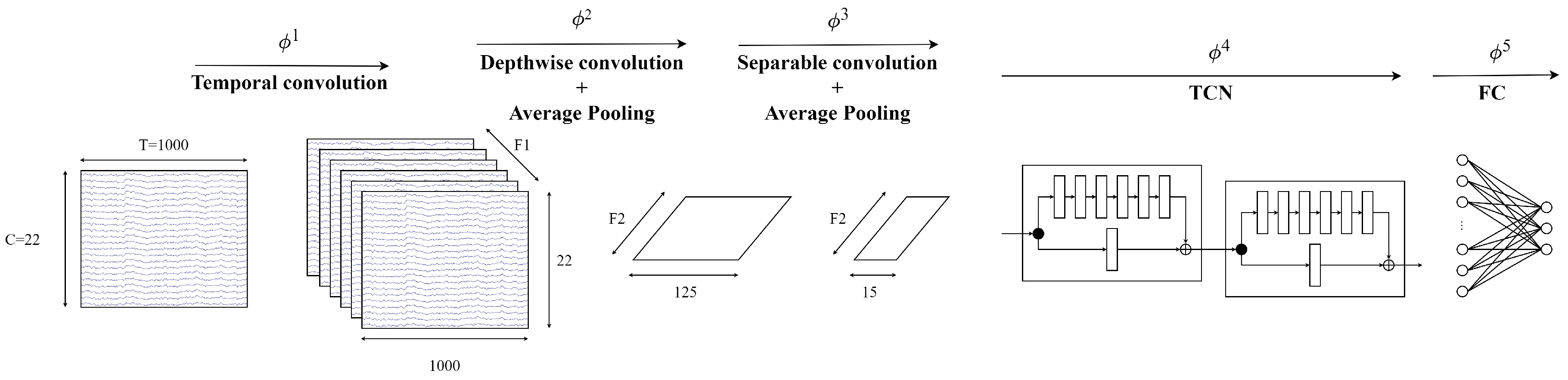
Figure 6 visualises the architecture of EEG-TCNet. EEG-TCNet has a temporal convolution module, depthwise convolution, separable convolution, TCN, and a fully connected network. Two-dimensional temporal convolution learns the frequency information, and then feature maps are extracted from the frequency-specific spatial information by depthwise convolution before the temporal summary for each feature map is learned by separable convolution. The TCN continues to extract the temporal information from feature maps after separable convolution and, finally, classification by the fully connected network.
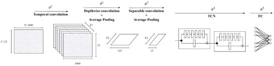
Figure 6.
Architecture of EEG-TCNet [18].
3.4. EEG-Conformer
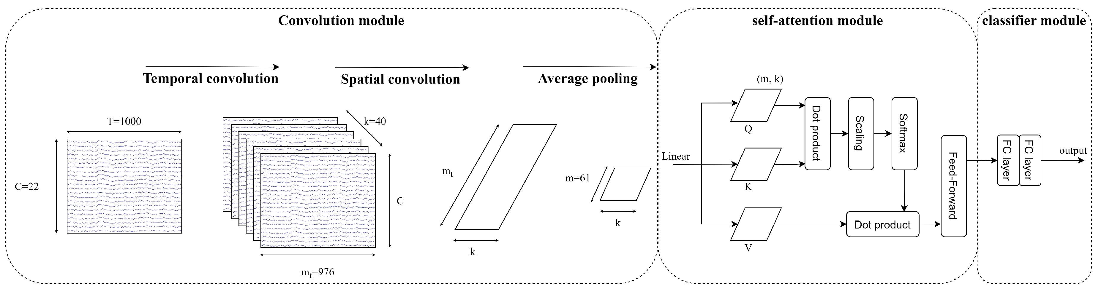
The second model in this study is EEG-Conformer, proposed by Song [26], based on the concept of using CNN to learn the low-level temporal and spatial features in EEG signals combined with self-attention to learn the global temporal dependencies in EEG feature maps. EEG-Conformer could be described in detail as follows:
- (a)
- Convolution module: The EEG signals after preprocessing and augmenting are learned through two 1D temporal and spatial convolution layers. The first temporal convolution layer learns the time dimension of input, and then the spatial convolution layer learns the spatial features. The spatial features are the information between the electrode channels. Then, the feature maps go through batch normalisation to avoid overfitting and the nonlinearity activation function ELU. The average pooling layer smooths the feature maps and rearranges to put all feature channels of each temporal point as a token into the self-attention module.
- (b)
- Self-attention module: The self-attention module has advantages in learning global features and long sequence data, which improve the CNN weaknesses. The self-attention module calculates as below:where Q is a matrix of stacked temporal queries, K and V are temporal matrices that denote key and value, and k is the length of tokens.Multi-head attention (MHA) is applied to strengthen representation performance. The tokens are separated into the same shape h segments, described as follows:where MHA is the multi-head attention , indicating the query, key, and value acquired by a linear transformation of a segment token in the lth head, respectively.
- (c)
- Classifier module: The features from the self-attention module go through two fully connected layers. The Softmax function is utilised to predict M labels. Cross-entropy loss is utilised as a cost function as follows:where is the batch size, M is the number of target labels (M = 4), y is the ground truth, and is the prediction.
Figure 7 visualises the architecture of an EEG-Conformer architecture. The network starts with a shallow convolution module; temporal information of the input is extracted by temporal convolution, and then the spatial information is extracted by spatial convolution. After that, the global temporal dependencies in feature maps are learned by the self-attention module. Finally, the classifier module, including fully connected networks, produces the prediction.
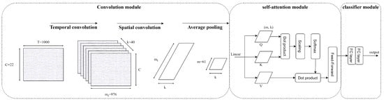
Figure 7.
Architecture of EEG-Conformer [26].
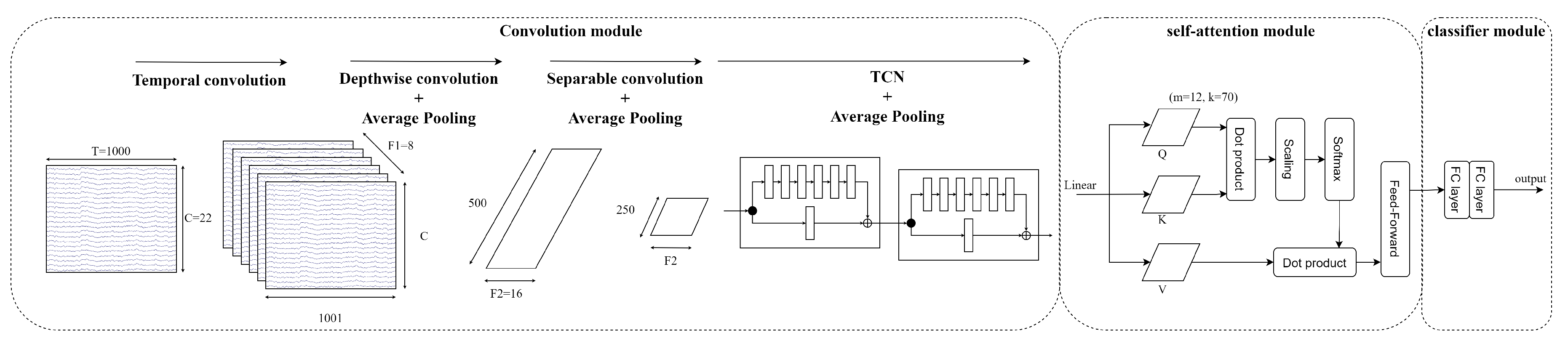
3.5. EEG-TCNTransformer
The concept of EEG-TCNTransformer is inspired by EEG-TCNet and EEG-Conformer. EEG-TCNet performs well in learning the local features in EEG signals because of the EEGNet and TCN modules. Besides that, EEG-Conformer solves the problem of global feature dependencies, which improves the learning of long sequence inputs. EEG-TCNTransformer has a convolution module, self-attention module, and classifier module.
- (a)
- Convolution module: The sequence of a 2D convolution layer, depthwise convolution layer, separable convolution layer, and average pooling layer extracts the temporal and spatial information in EEG signals. After that, a sequence of TCN blocks continues to learn large receptive fields efficiently with small parameters because of dilated causal convolution and a residual block structure. In this study, the different numbers of filters k in a TCN block and the numbers of a TCN block T are validated to select the best hyperparameter for EEG-TCNTransformer. Then, the average pooling layer smooths the features and rearranges the features to the shape of channels of each temporal point.
- (b)
- Self-attention module: Six self-attention blocks with a multi-head attention architecture learn the global temporal dependencies in features from the convolution module. The self-attention module calculates as below:where Q is a matrix of stacked temporal queries, K and V are temporal matrices that denote key and value, and k is the length of tokens.Multi-head attention (MHA) is applied to strengthen representation performance. The tokens are separated into the same shape h segments, described as follows:where MHA is the multi-head attention , indicating the query, key, and value acquired by a linear transformation of a segment token in the lth head, respectively.
- (c)
- Classifier module: Two fully connected layers transform the features into M labels that calculate probability distribution by the Softmax function. The loss function is the cross-entropy loss, as follows:where is the batch size, M is the number of target labels (M = 4), y is the ground truth, and is the prediction.
Figure 8 visualises the architecture of an EEG-TCNTransformer architecture. Instead of a shallow convolution module in EEG-Conformer, the temporal convolution, depthwise convolution, and separable convolution are used to extract the temporal information, frequency-temporal information, and temporal summary from feature maps. The TCN module exploits the temporal features from feature maps before the global temporal dependencies are learned by the self-attention module. Finally, the classification is produced by the classifier module.
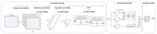
Figure 8.
Architecture of EEG-TCNTransformer.
4. Experiments and Results
4.1. Experimental Setup
The training environment was set up on a Linux computer with CPU AMD Ryzen 9 5900X, GPU RTX 3080, and CUDA 12.1. EEG-TCNet was implemented in the Python 3.6.8 code using TensorFlow. EEG-Conformer and EEG-TCNTransformer were implemented in the Python 3.10.14 code using PyTorch. The Conda environment is used in this experiment to change the Python version.
4.2. Training and Testing Preparation
A four-class motor imagery (001-2014) dataset can be retrieved from https://bnci-horizon-2020.eu/database/data-sets (accessed on 17 September 2024); there are 18 data files for 9 subjects, so 1 subject has 1 training data file ending with T (A01T, A02T, A03T, …) and 1 testing data file ending with E (A01E, A02E, A03E, …). Before training, there are 2 different data preparation procedures:
- Without a bandpass filter, data are loaded from Matlab files, and for each trial, , which is equivalent to 4 s from the cue section to the end of the motor imagery section.
- With a bandpass filter, data are exactly the same as above; then the data are processed by a bandpass filter step with the order of the filter N and the minimum attenuation required in the stop band .
The data preparation without a bandpass filter is utilised for training and evaluating models with different hyperparameters; then the data preparation with a bandpass filter is utilised for evaluating the influence of different bandpass filters on models’ performance. After the data preparation stage, the processed data are trained with 3 models, EEG-TCNet, EEF-Conformer, and EEG-TCNTransformer. For each model, there are different configurations, as follows:
- Regarding EEG-TCNet, each subject is trained with 1000 epochs with a learning rate of 0.001, the criterion is categorical cross-entropy, the optimiser is Adam, and the activation function is ELU.
- With regard to EEG-Conformer, each subject is trained with 2000 epochs with a learning rate of 0.0002, the criterion is cross-entropy, the optimiser is Adam, the activation function in the convolution module and classification module is ELU, and the activation function in self-attention blocks is GELU.
- With respect to EEG-TCNTransformer, each subject is trained 5000 epochs with a learning rate of 0.0002, the criterion is cross-entropy, the optimiser is Adam, the activation function in EEGNet module, TCN module and classification module is ELU, and the activation function in self-attention blocks is GELU.
The accuracy metric is utilised to measure the performance.
4.3. EEG-TCNet with Different Hyperparameters
The detailed architecture of EEG-TCNet is described in Table 1. C and T denote the number of EEG channels and the number of time points. In the first sub-project, and because the time points used in training are 4 s from the cue section to the end of the motor imagery section. The baseline hyperparameters of EEG-TCNet are , the same as those for the authors. Besides that, the dropout values in the EEGNet module and the TCN module are , the same as in the original paper. Where is dropout in EEGNet module and is dropout in TCN module.

Table 1.
EEG-TCNet architecture [18].
In the first sub-project, EEG-TCNet is trained with different numbers of filters and kernel sizes in the EEGNet module and TCN module, as described in Table 2.
Table 2.
Experiment EEG-TCNet with different hyperparameters.
In Table 3, the contribution of each to the performance of EEG-TCNet is examined by keeping the baseline value of three parameters and changing one parameter. The average accuracy of EEG-TCNet increases when and increase. The average accuracy of EEG-TCNet drops when it increases to 12 while increasing to 14 improves the average accuracy of EEG-TCNet. Increasing to 6 also improve the accuracy, but the performance declines when increasing to 8. The detailed accuracy of 9 subjects is in Table A1.
Table 3.
Comparison of different numbers of filters and kernel sizes in the EEGNet module and the TCN module in average accuracy.
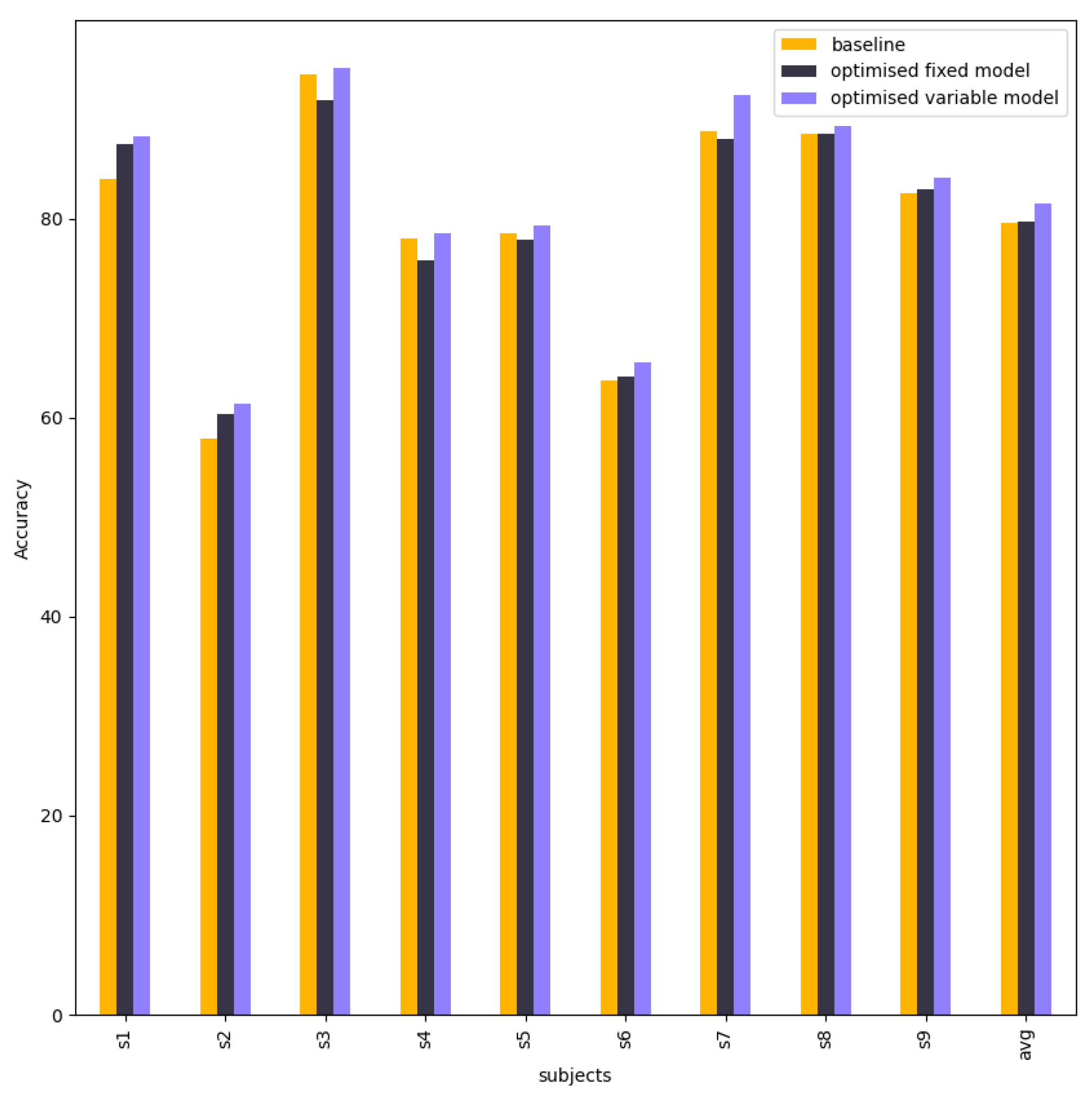
After training 81 experiments, a fixed result and a variable result are selected. In terms of the fixed result, the best hyperparameters for all 9 subjects are selected based on the average accuracy. Regarding the variable result, the best hyperparameters for each subject are selected. Table 4 shows the hyperparameters of the variable model.
Table 4.
Variable hyperparameters of EEG-TCNet.
Table 5 compares the accuracies between the baseline model, fixed model, and variable model. The fixed model is better than the baseline model in subject 2, subject 4, subject 6, and subject 9, whereas others are nearly equal. When each subject is selected as the best result in the variable model, the final performance is much higher than the baseline model, especially for subject 2, subject 4, subject 5, subject 6, and subject 9.
Table 5.
Accuracy of the EEG-TCNet baseline model, fixed model, and variable models (%).
Figure 9 shows a column chart of a comparison in accuracy between baseline EEG-TCNet, EEG-TCNet with the best tuning hyperparameters (optimised fix model), and EEG-TCNet with the best hyperparameters of each subject from different trainings. This experiment aims to research the impact of different hyperparameters on EEG-TCNet. The variable model is obviously better than the baseline and fixed model because each subject is the best hyperparameter from numerous training experiments.
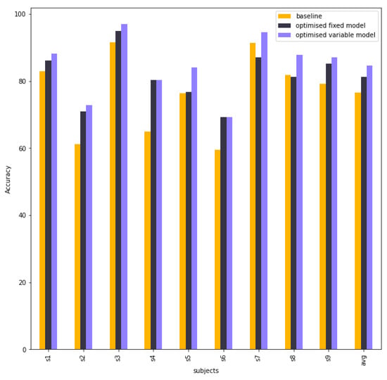
Figure 9.
The column chart shows the accuracy between the EEG-TCNet baseline model, fixed model, and variable model.
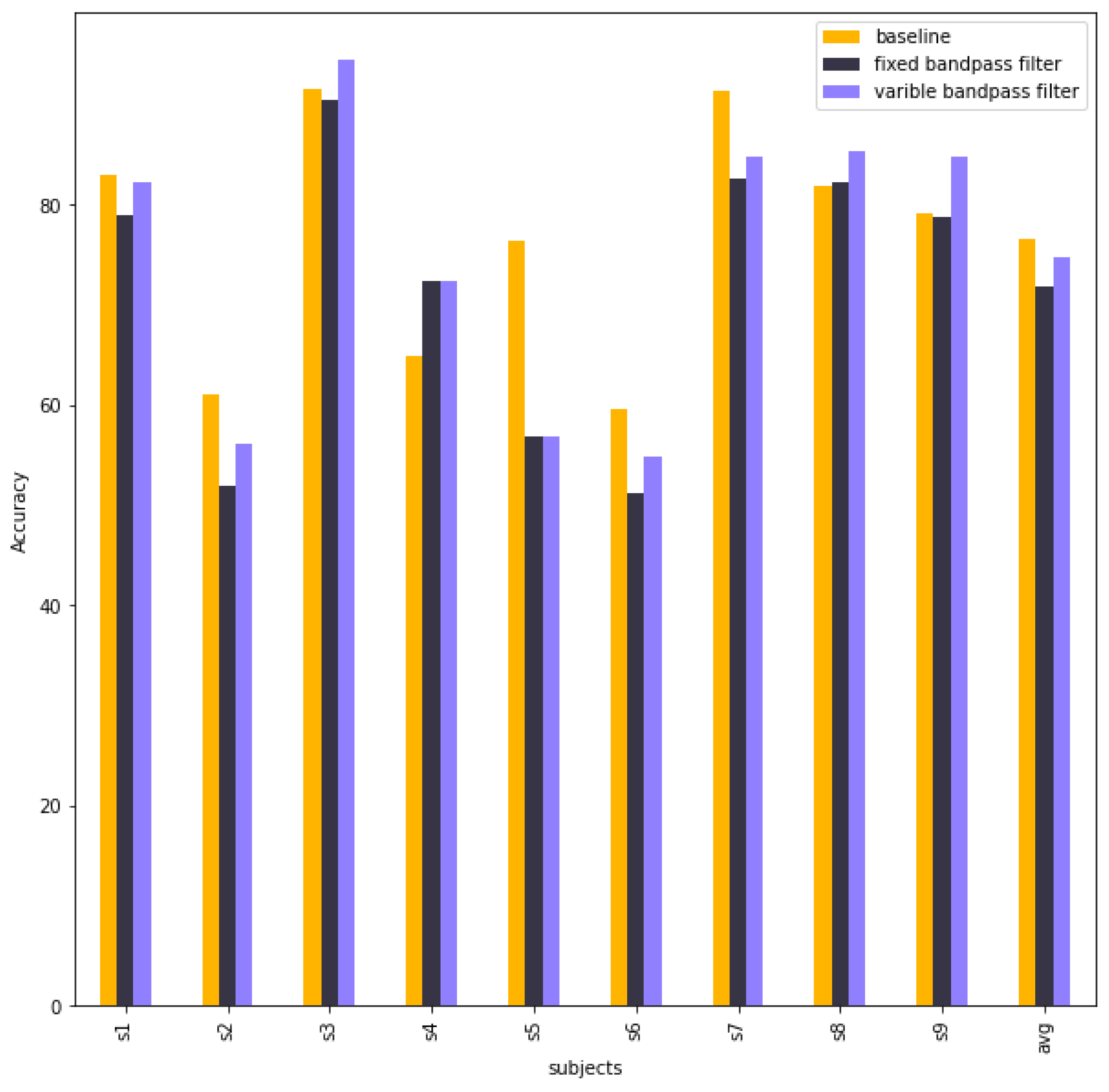
4.4. EEG-TCNet with Different Bandpass Filter Parameters
In sub-project 2, EEG-TCNet with baseline hyperparameters is trained with different orders of the filter and the minimum attenuations required in the stop band of Chebyshev type 2, described in Table 6. The parameters N and are defined in cheby2 of SciPy API for Python (3.12.5).
Table 6.
Experiment EEG-TCNet with different parameters of Chebyshev type 2 filter.
After training 45 experiments, a fixed result and a variable result are selected. With regard to the fixed result, the best Chebyshev type 2 parameters for all 9 subjects are selected based on the average accuracy. Regarding the variable result, the best Chebyshev type 2 parameters N, for each subject are selected. Table 7 summarises the variable result.
Table 7.
Variable bandpass filter of EEG-TCNet.
Table 8 compares the accuracy of 9 subjects and the average accuracy between baseline EEG-TCNet, EEG-TCNet with a fixed bandpass filter, and EEG-Net with a variable bandpass filter. The performance of EEG-TCNet decreased after using Chebyshev type 2 in preprocessing in both a fixed bandpass filter and a variable bandpass filter. The detailed accuracy of 9 subjects is in Table A2.
Table 8.
Accuracy of baseline EEG-TCNet and EEG-TCNet with fixed bandpass filter and with variable bandpass filter (%).
Figure 10 shows a comparison of accuracies between baseline EEG-TCNet, EEG-TCNet with the best bandpass filter parameters (fixed bandpass filter), and EEG-TCNet with the best bandpass filter parameters of each subject from different trainings. This experiment aims to research the impact of different bandpass filter parameters on EEG-TCNet. Figure 10 shows that the bandpass filter does not improve the performance of EEG-TCNet.
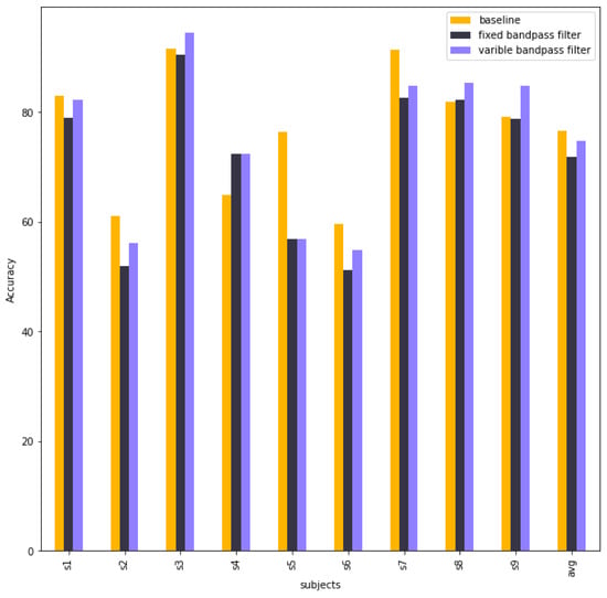
Figure 10.
The column chart shows the accuracies of baseline EEG-TCNet, EEG-TCNet with a fixed bandpass filter, and EEG-TCNet with a variable bandpass filter.
4.5. EEG-Conformer with Different Hyperparameters
The architecture of the convolution module of EEG-Conformer is described in Table 9.
Table 9.
The architecture of the convolution module in EEG-Conformer [26].
In sub-project 1 with EEG-Conformer, the model is trained with different numbers of temporal filters in convolution module k and different numbers of self-attention blocks N, described in Table 10. The baseline model in the original study has and .
Table 10.
Experiment EEG-Conformer with different hyperparameters.
In Table 11, the contribution of each to the performance of EEG-TCNet is examined by keeping the baseline value of one parameter and changing one parameter. The increasing k improves the average accuracy, but the performance declines when k rises from 40 to 60. The average accuracy decreases when N is from 6 to 7 and then increases slightly when N is from 7 to 10, but the average accuracy is still lower than N of 6. The detailed accuracy of 9 subjects is in Table A3.
Table 11.
Comparison of different numbers of filters k and numbers of self-attention blocks N in EEG-Conformer in average accuracy.
After training 25 experiments, the fixed hyperparameters selected are and . The variable hyperparameters are described in Table 12.
Table 12.
Variable hyperparameters of EEG-Conformer.
Table 13 compares and visualises the accuracies of the EEG-Conformer baseline model, fixed model, and variable models. Their accuracies are nearly equal in each subject. However, subject 2 in the fixed model has higher accuracy than that in the baseline model.
Table 13.
Accuracies of the EEG-Conformer baseline model, fixed model, and variable models.
Figure 11 shows a comparison of accuracies between baseline EEG-Conformer, EEG-Conformer with the best tuning hyperparameters (optimised fix model), and EEG-Conformer with the best hyperparameters of each subject from different trainings. This experiment aims to research the impact of different hyperparameters on EEG-Conformer. This is evidence that different hyperparameters do not enhance EEG-Conformer.
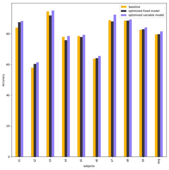
Figure 11.
The column chart shows the accuracy between the EEG-Conformer baseline model, fixed model, and variable.
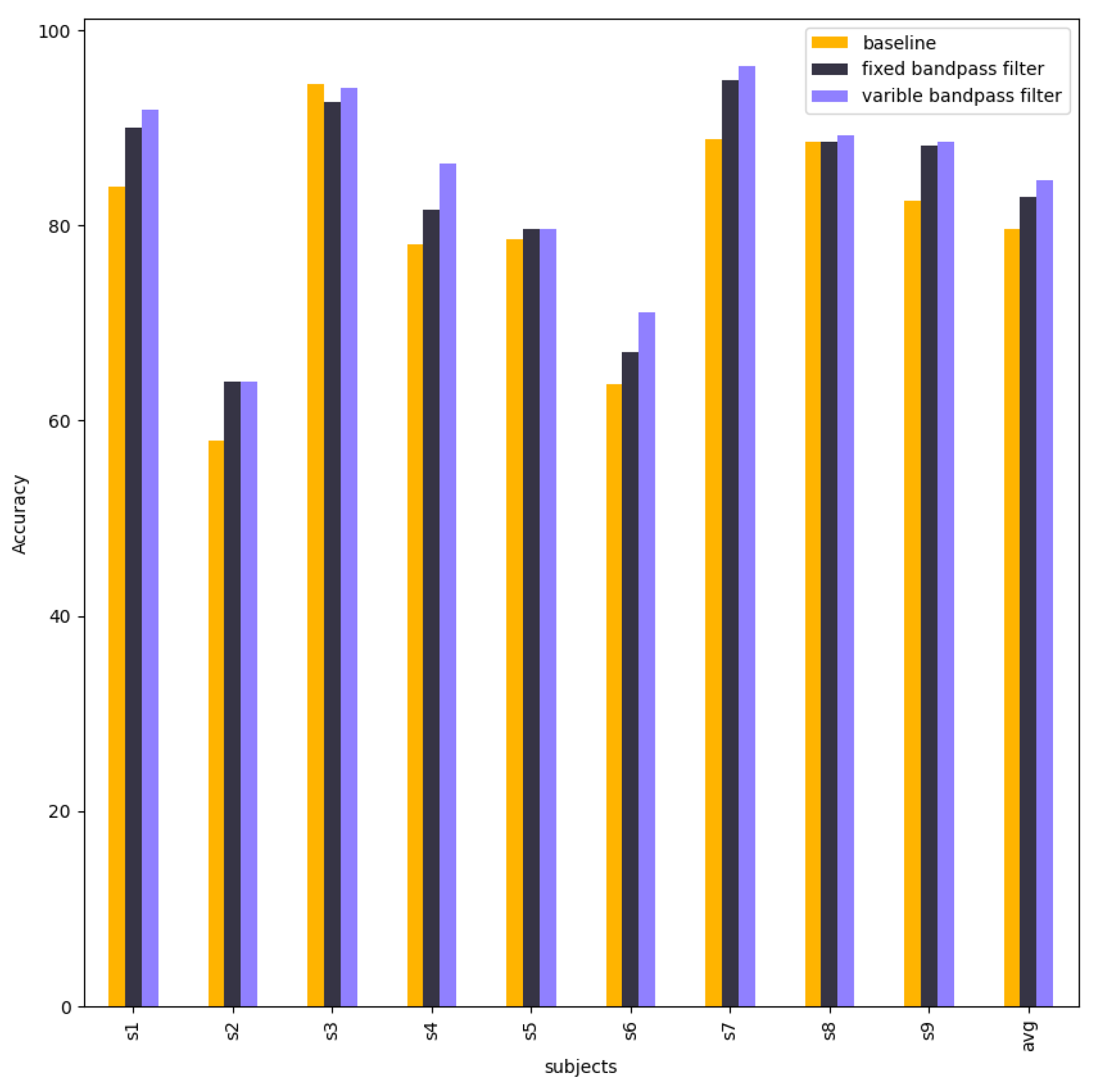
4.6. EEG-Conformer with Different Bandpass Filter Parameters
In the second sub-project with EEG-Conformer, the baseline model is trained with different orders of the filter and the minimum attenuations required in the stop band of Chebyshev type 2, as described in Table 14.
Table 14.
Experiment EEG-Conformer with different parameters of Chebyshev type 2 filter.
After training 45 experiments, a fixed result and a variable result are selected. With regard to the fixed result, the best Chebyshev type 2 parameters for all 9 subjects are selected based on the average accuracy. Regarding the variable result, the best Chebyshev type 2 parameters for each subject are selected. Table 15 summarises the variable result.
Table 15.
Variable bandpass filter of EEG-Conformer.
Table 16 compares and visualises the accuracies of baseline EEG-Conformer, EEG-Conformer with a fixed bandpass filter, and EEG-Conformer with a variable bandpass filter. Chebyshev type 2 contributes to improving the accuracy of subject 1, subject 2, subject 4, and subject 7. Other subjects are approximate to the baseline model. The variable result obtained an average accuracy of 84.61%. The detailed accuracy of 9 subjects is in Table A4.
Table 16.
Accuracy of baseline EEG-Conformer, EEG-Conformer with a fixed bandpass filter, and EEG-Conformer with a variable bandpass filter (%).
Figure 12 shows a comparison of accuracies between baseline EEG-Conformer, EEG-Conformer with the best bandpass filter parameters (fixed bandpass filter), and EEG-Conformer with the best bandpass filter parameters of each subject from different trainings. This experiment aims to research the impact of different bandpass filter parameters on EEG-Conformer. The improvement in accuracy shows that the bandpass filter contributes to the robustness of EEG-Conformer.

Figure 12.
The column chart shows the accuracies of baseline EEG-Conformer, EEG-Conformer with a fixed bandpass filter, and EEG-Conformer with a variable bandpass filter.
4.7. EEG-TCNTransformer with Different Hyperparameters
The different number of filters k in the TCN block and number of TCN blocks T are validated to select the best hyperparameters. In Table 17, the average of all subjects is summarised with different k and T. With each T, the more filters k, the higher the average accuracy, but the average accuracy stops increasing and decreases at a level of filters. With , the average accuracy is highest at k = 60. With , the average accuracy is highest at k = 60. With , the average accuracy is highest at k = 70. Overall, and produce the best average accuracy of 83.41%. The detailed accuracy of 9 subjects is in Table A5.
Table 17.
The average accuracy of different numbers of filters k and the number of TCN blocks T.
In Table 18, the most improvement is seen in subject 2; EEG-TCNTransformer is higher than EEG-Conformer by about 10.95% and higher than EEG-TCNet by about 7.77%. Subject 6 and subject 9 of EEG-TCNTransformer are also more improved significantly than those of EEG-Conformer, by about 4.65% and 6.44%, respectively. Additionally, EEG-TCNTransformer improves subject 1 and subject 4 by about 3.91% and 3.95%, respectively. The average accuracy of EEG-TCNTransformer is 83.41% (confidence interval = 95.2%), which is higher by 3.77% than the average accuracy of EEG-Conformer and 6.86% than the average accuracy of EEG-TCNet.
Table 18.
Comparisons in the accuracy EEG-TCNet baseline, EEG-Conformer baseline, and EEG-TCNTransformer.
In Table 19, EEG-TCNTransformer improves subject 2 by about 11.16% compared with EEG-Conformer, but only higher by 2.59% than EEG-TCNet. Subject 9 of EEG-TCNTransformer has the highest improvement in precision, about 6.44% and 9.85% compared with EEG-Conformer and EEG-TCNet, respectively. Moreover, EEG-TCNTransformer also improves the precision of subject 1, subject 4, subject 5, and subject 6 compared with both EEG-TCNet and EEG-Conformer. The average precision of EEG-TCNTransformer is 83.43%, which is higher by 3.77% than the average precision of EEG-Conformer and 4.36% than the average precision of EEG-TCNet.
Table 19.
Comparisons in the precision of baseline EEG-TCNet, baseline EEG-Conformer, and EEG-TCNTransformer.
In Table 20, the recall of subject 2 of EEG-TCNTransformer is significantly higher than that of EEG-Conformer by 12.62% and higher than that of EEG-TCNet by 9.97%. Moreover, EEG-TCNTransformer improves the recall of subject 6 and subject 9 by about 6.49% and 5.28% compared with EEG-Conformer. Additionally, EEG-TCNTransformer also improves the recall of subject 1, subject 4, and subject 5. The average recall of EEG-TCNTransformer is 84.05%, which is higher by 3.89% than the average recall of EEG-Conformer and 7.49% than the average recall of EEG-TCNet.
Table 20.
Comparisons in the recall of baseline EEG-TCNet, baseline EEG-Conformer, and EEG-TCNTransformer.
Table 21 is a comparison table of F1 score between baseline EEG-TCNet, baseline EEG-Conformer, and EEG-TCNTransformer. EEG-TCNTransformer improves the F1 score of subject 2 by about 10.23% and 6.67% compared with EEG-Conformer and EEG-TCNet, respectively. Moreover, EEG-TCNTransformer improves the F1 score of subject 1, subject 4, subject 5, subject 6, and subject 9 from 3.2% up to 4.44%. The average F1 score of EEG-TCNTransformer is 83.25%, which is higher by 3.63% than the average F1 score of EEG-Conformer and 7.23% than the average F1 score of EEG-TCNet.
Table 21.
Comparisons of the F1 scores of baseline EEG-TCNet, baseline EEG-Conformer, and EEG-TCNTransformer.
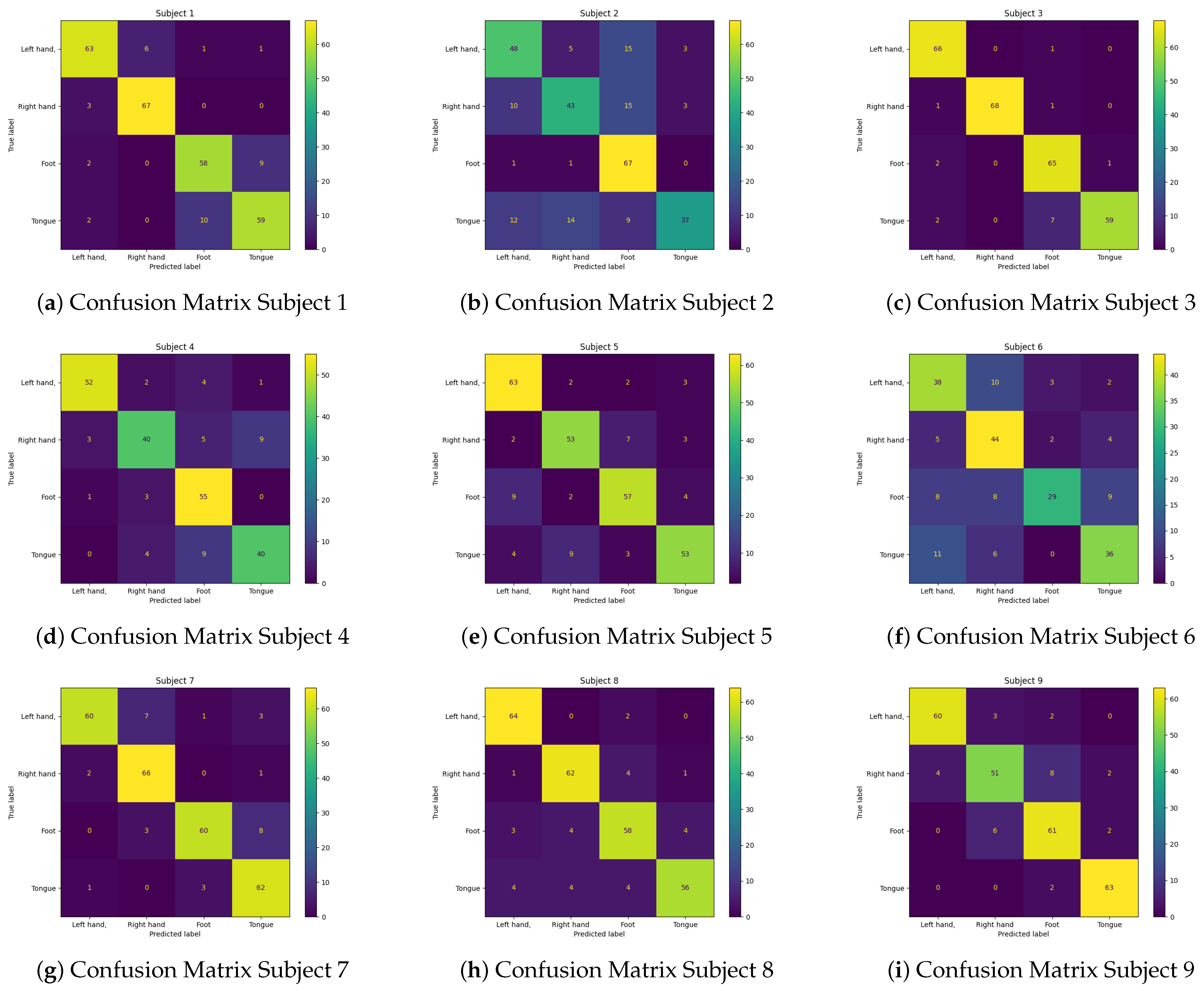
Besides that, Figure 13 provides the confusion matrices of 9 subjects of EEG- TCNTransformer below. Models of subject 3, subject 4, subject 5, subject 7, subject 8, and subject 9 perform well in classifying 4 classes: left hand, right hand, foot, and tongue. Subject 1 has an incorrect classification of about 9 to 10 samples in the foot and tongue classes. Subject 2 has some incorrect classifications between the tongue and other classes and between the foot and other classes. Subject 6 also has some incorrect classifications in the left hand and other classes and between the right hand and other classes.

Figure 13.
Confusion Matrix of EEG-TCNTransformer model for 9 subjects.
-2.2in
4.8. EEG-TCNTransformer with Different Bandpass Filter Parameters
The bandpass filter is also added to the preprocessing to validate the performance of EEG-TCNTransformer. Table 22 describes the average accuracy of different orders of the filter N = (1, 2, 3, 4, 5, 6, 7, 8, 9, 10) with the minimum attenuations required in the stop band = (10, 20, 30). The highest average accuracy when training EEG-TCNTransformer with a bandpass filter is 80.27%, while increasing reduces the performance (Table A6). Therefore, the bandpass filter is inefficient for EEG-TCNTransformer.
Table 22.
The average accuracy of EEG-TCNTransformer with different bandpass filter parameters.
5. Discussion
This research aims to study the contribution of changing hyperparameters and changing bandpass filter parameters of Chebyshev type 2 to a CNN method and a Transformer method in brain–computer interface motor imagery. Regarding the CNN method, EEG-TCNet is a novel study for research. The increase in the number of filters and kernel sizes in EEG-TCNet architecture provides better performance. However, the bandpass filter Chebyshev type 2 in data preprocessing is inefficient for training EEG-TCNet. In terms of the Transformer method, EEG-Conformer is chosen for this research. The average accuracy improves when the number of filters is between 20 and 40. The Chebyshev type 2 bandpass filter was found to contribute significantly to the accuracy of each subject, producing an average accuracy of 83.41%. However, EEG-TCNet still has other hyperparameters, such as dropout, depth of TCN blocks, depth in EEGNet module, or EEG-Conformer, still having dropout and head number in multi-head that cannot be examined in this study because of the limit of training resource and time.
In this research, a new model called EEG-TCNTransformer is created, which combines the convolution parts of EEG-TCNet and the sequence of self-attention blocks. The average accuracy of EEG-TCNTransformer improves when the number of TCN blocks increases, which learns better the low-level temporal features in temporal and spatial features. The number of filters also contributes to the performance, but it gets overfitting at specific filters. Moreover, the bandpass filter is inefficient for EEG-TCNTransformer, so the raw EEG data with standardisation are used in training and testing. Therefore, the optimised hyperparameters for EEG-TCNTransformer generate better accuracy for each subject compared with baseline EEG-TCNet and baseline EEG-Conformer without a bandpass filter in preprocessing, and the average accuracy of EEG-TCNTransformer is 83.41%.
6. Conclusions
Brain–computer interface motor imagery is an emerging research topic in artificial intelligence. This study explores the contributions of hyperparameters and bandpass filters to the performance of EEG-TCNet and EEG-Conformer. The average accuracy of EEG-TCNet is improved when increasing the number of filters and kernel size, but the bandpass filter is inefficient in training. In contrast, the bandpass filter significantly improves the accuracy of EEG-Conformer, where the performance is unimproved when increasing the number of self-attention blocks. Furthermore, a new model, EEG-TCNTransformer, incorporates the convolution architecture of EEG-TCNet and a stack of self-attentions with a multi-head structure. This EEG-TCNTransformer outperforms with an average accuracy of 83.41%. In future, various techniques within the transformer architecture will be explored to enhance the global feature correlation for EEG-TCNTransformer.
Author Contributions
Conceptualisation, A.H.P.N. and O.O.; methodology, A.H.P.N. and O.O.; software, A.H.P.N.; validation, A.H.P.N.; formal analysis, A.H.P.N.; investigation, A.H.P.N. and O.O.; resources, A.H.P.N.; data curation, A.H.P.N.; writing—original draft preparation, A.H.P.N. and O.O.; writing—review and editing, A.H.P.N., O.O., M.A.P. and S.H.L.; visualisation, A.H.P.N.; supervision, M.A.P. and S.H.L.; project administration, M.A.P. and S.H.L. All authors have read and agreed to the published version of the manuscript.
Funding
This research received no external funding.
Institutional Review Board Statement
This study’s EEG dataset is already accessible in the BNCI Horizon 2020 database. Ethical review and approval were waived for this study, due to the use of publicly available datasets.
Informed Consent Statement
This study used publicly available dataset where informed consent was obtained from all subjects involved in the study.
Data Availability Statement
The data are available in the BNCI Horizon 2020 database found on this link: https://bnci-horizon-2020.eu/database/data-sets (accessed on 17 September 2024).
Conflicts of Interest
The authors declare no conflicts of interest.
Appendix A. TCNet Training Results
Appendix A.1. Experiment EEG-TCNet with Different Hyperparameters
Table A1 shows the accuracy of 9 subjects when changing in EEG-TCNet architecture.
Table A1.
Accuracy of EEG-TCNet with different .
Table A1.
Accuracy of EEG-TCNet with different .
| S1 | S2 | S3 | S4 | S5 | S6 | S7 | S8 | S9 | Average Accuracy (%) | ||||
|---|---|---|---|---|---|---|---|---|---|---|---|---|---|
| 6 | 16 | 10 | 4 | 79.36 | 59.36 | 91.21 | 67.11 | 75.72 | 56.28 | 75.09 | 81.92 | 75.00 | 73.45 |
| 6 | 16 | 10 | 6 | 82.21 | 60.07 | 94.51 | 72.37 | 75.72 | 62.33 | 76.17 | 84.13 | 79.55 | 76.34 |
| 6 | 16 | 10 | 8 | 82.92 | 59.72 | 95.24 | 74.56 | 75.72 | 66.98 | 81.23 | 82.66 | 76.52 | 77.28 |
| 6 | 16 | 12 | 4 | 80.78 | 66.43 | 93.77 | 66.23 | 77.90 | 58.14 | 93.14 | 83.03 | 82.95 | 78.04 |
| 6 | 16 | 12 | 6 | 80.43 | 60.78 | 93.77 | 76.75 | 80.80 | 64.19 | 88.45 | 83.03 | 83.33 | 79.06 |
| 6 | 16 | 12 | 8 | 83.63 | 67.49 | 91.21 | 67.98 | 80.80 | 65.12 | 76.53 | 83.76 | 84.47 | 77.89 |
| 6 | 16 | 14 | 4 | 75.09 | 53.00 | 88.28 | 67.11 | 75.72 | 54.88 | 76.17 | 81.55 | 75.00 | 71.87 |
| 6 | 16 | 14 | 6 | 78.65 | 61.48 | 89.38 | 73.68 | 75.72 | 64.65 | 92.78 | 82.29 | 76.89 | 77.28 |
| 6 | 16 | 14 | 8 | 82.56 | 60.42 | 95.60 | 74.12 | 75.72 | 68.84 | 92.06 | 76.75 | 76.14 | 78.02 |
| 6 | 32 | 10 | 4 | 76.51 | 63.96 | 91.21 | 72.37 | 79.35 | 53.49 | 75.09 | 82.29 | 75.38 | 74.40 |
| 6 | 32 | 10 | 6 | 82.21 | 68.20 | 94.51 | 65.35 | 76.09 | 64.65 | 91.34 | 80.07 | 80.68 | 78.12 |
| 6 | 32 | 10 | 8 | 76.16 | 57.95 | 95.24 | 75.44 | 78.99 | 63.26 | 88.09 | 86.72 | 85.23 | 78.56 |
| 6 | 32 | 12 | 4 | 81.49 | 56.89 | 91.58 | 70.18 | 72.10 | 61.40 | 77.62 | 82.66 | 84.47 | 75.38 |
| 6 | 32 | 12 | 6 | 80.43 | 65.37 | 94.87 | 74.56 | 79.35 | 61.86 | 91.70 | 80.44 | 81.44 | 78.89 |
| 6 | 32 | 12 | 8 | 82.56 | 56.18 | 93.41 | 75.88 | 78.62 | 61.40 | 91.70 | 84.87 | 85.98 | 78.96 |
| 6 | 32 | 14 | 4 | 83.63 | 59.01 | 94.51 | 67.98 | 70.65 | 60.00 | 90.25 | 78.60 | 79.17 | 75.98 |
| 6 | 32 | 14 | 6 | 76.16 | 61.84 | 97.07 | 80.26 | 73.55 | 60.93 | 81.23 | 83.76 | 81.82 | 77.40 |
| 6 | 32 | 14 | 8 | 85.05 | 66.78 | 91.21 | 71.49 | 75.36 | 60.93 | 87.73 | 77.86 | 76.89 | 77.03 |
| 6 | 48 | 10 | 4 | 87.54 | 63.96 | 93.41 | 70.61 | 75.36 | 57.67 | 75.81 | 82.66 | 78.03 | 76.12 |
| 6 | 48 | 10 | 6 | 79.36 | 59.36 | 89.74 | 70.61 | 76.45 | 65.58 | 90.25 | 83.39 | 79.17 | 77.10 |
| 6 | 48 | 10 | 8 | 78.65 | 63.25 | 93.04 | 72.81 | 81.16 | 63.26 | 91.70 | 81.92 | 82.95 | 78.75 |
| 6 | 48 | 12 | 4 | 78.65 | 51.94 | 91.94 | 69.30 | 73.91 | 64.65 | 84.12 | 81.92 | 83.71 | 75.57 |
| 6 | 48 | 12 | 6 | 88.26 | 64.66 | 97.07 | 63.60 | 79.35 | 63.26 | 90.97 | 81.55 | 81.82 | 78.95 |
| 6 | 48 | 12 | 8 | 83.27 | 61.84 | 94.87 | 77.63 | 79.71 | 66.51 | 76.17 | 83.39 | 82.20 | 78.40 |
| 6 | 48 | 14 | 4 | 79.00 | 57.95 | 91.21 | 70.18 | 71.38 | 59.53 | 90.25 | 84.13 | 81.06 | 76.08 |
| 6 | 48 | 14 | 6 | 77.22 | 56.54 | 93.04 | 71.93 | 78.99 | 61.86 | 76.90 | 84.13 | 79.55 | 75.57 |
| 6 | 48 | 14 | 8 | 83.27 | 65.72 | 92.67 | 76.32 | 77.54 | 57.67 | 78.34 | 81.92 | 80.30 | 77.08 |
| 8 | 16 | 10 | 4 | 79.36 | 62.54 | 89.74 | 71.05 | 72.46 | 60.00 | 90.25 | 85.98 | 83.33 | 77.19 |
| 8 | 16 | 10 | 6 | 82.21 | 67.14 | 95.24 | 69.30 | 76.45 | 67.91 | 90.61 | 82.29 | 80.68 | 79.09 |
| 8 | 16 | 10 | 8 | 83.27 | 67.49 | 94.14 | 76.32 | 80.43 | 66.51 | 91.34 | 80.07 | 75.76 | 79.48 |
| 8 | 16 | 12 | 4 | 82.92 | 60.78 | 93.04 | 67.98 | 66.30 | 62.79 | 93.14 | 80.81 | 82.20 | 76.66 |
| 8 | 16 | 12 | 6 | 81.49 | 66.43 | 93.41 | 70.61 | 77.17 | 64.65 | 88.81 | 84.50 | 85.23 | 79.15 |
| 8 | 16 | 12 | 8 | 82.21 | 67.49 | 94.14 | 78.07 | 73.91 | 67.44 | 88.45 | 83.76 | 85.61 | 80.12 |
| 8 | 16 | 14 | 4 | 78.65 | 57.60 | 88.64 | 66.23 | 80.43 | 60.47 | 92.78 | 84.13 | 82.20 | 76.79 |
| 8 | 16 | 14 | 6 | 79.72 | 67.14 | 93.04 | 68.86 | 80.43 | 55.81 | 88.81 | 83.39 | 79.17 | 77.37 |
| 8 | 16 | 14 | 8 | 81.14 | 61.13 | 92.67 | 75.88 | 79.35 | 66.51 | 88.09 | 79.70 | 80.68 | 78.35 |
| 8 | 32 | 10 | 4 | 85.77 | 65.72 | 95.24 | 75.88 | 76.09 | 56.74 | 88.81 | 81.92 | 75.76 | 77.99 |
| 8 | 32 | 10 | 6 | 82.56 | 67.49 | 93.77 | 78.51 | 79.71 | 64.65 | 90.25 | 85.61 | 84.85 | 80.82 |
| 8 | 32 | 10 | 8 | 82.56 | 65.72 | 94.14 | 76.32 | 84.06 | 65.58 | 92.42 | 84.13 | 86.36 | 81.26 |
| 8 | 32 | 12 | 4 | 82.92 | 61.13 | 91.58 | 64.91 | 76.45 | 59.53 | 91.34 | 81.92 | 79.17 | 76.55 |
| 8 | 32 | 12 | 6 | 83.63 | 66.43 | 94.87 | 75.00 | 75.72 | 66.51 | 87.73 | 85.24 | 84.47 | 79.96 |
| 8 | 32 | 12 | 8 | 82.92 | 61.48 | 94.51 | 73.68 | 79.35 | 65.12 | 91.34 | 76.75 | 82.20 | 78.59 |
| 8 | 32 | 14 | 4 | 79.36 | 60.78 | 97.07 | 72.37 | 77.90 | 61.86 | 88.45 | 82.29 | 87.12 | 78.58 |
| 8 | 32 | 14 | 6 | 81.85 | 67.84 | 94.51 | 71.05 | 75.72 | 65.58 | 89.17 | 85.61 | 79.92 | 79.03 |
| 8 | 32 | 14 | 8 | 82.92 | 57.60 | 95.60 | 73.68 | 80.80 | 65.12 | 89.89 | 82.66 | 83.33 | 79.07 |
| 8 | 48 | 10 | 4 | 82.21 | 54.06 | 92.31 | 63.60 | 75.36 | 58.14 | 75.09 | 79.70 | 79.92 | 73.38 |
| 8 | 48 | 10 | 6 | 81.85 | 66.08 | 95.24 | 76.32 | 78.26 | 62.79 | 85.92 | 82.29 | 79.17 | 78.66 |
| 8 | 48 | 10 | 8 | 83.27 | 64.66 | 95.24 | 78.95 | 80.07 | 67.91 | 86.64 | 83.03 | 84.85 | 80.51 |
| 8 | 48 | 12 | 4 | 81.14 | 62.19 | 94.87 | 70.18 | 78.99 | 60.47 | 84.12 | 79.34 | 82.20 | 77.05 |
| 8 | 48 | 12 | 6 | 81.85 | 67.49 | 93.41 | 72.37 | 76.81 | 58.60 | 88.81 | 83.03 | 83.33 | 78.41 |
| 8 | 48 | 12 | 8 | 82.92 | 61.48 | 90.84 | 76.32 | 79.71 | 65.58 | 90.61 | 81.18 | 83.71 | 79.15 |
| 8 | 48 | 14 | 4 | 83.99 | 56.18 | 94.87 | 75.00 | 78.26 | 62.79 | 89.53 | 84.13 | 83.71 | 78.72 |
| 8 | 48 | 14 | 6 | 81.14 | 72.44 | 95.60 | 80.26 | 80.07 | 62.79 | 91.34 | 84.13 | 81.44 | 81.02 |
| 8 | 48 | 14 | 8 | 80.78 | 65.37 | 94.87 | 71.05 | 78.62 | 64.19 | 80.87 | 84.13 | 84.47 | 78.26 |
| 10 | 16 | 10 | 4 | 82.56 | 61.84 | 93.77 | 65.79 | 77.17 | 58.60 | 88.09 | 84.13 | 83.33 | 77.25 |
| 10 | 16 | 10 | 6 | 80.07 | 62.54 | 93.04 | 71.93 | 79.35 | 62.79 | 89.17 | 84.13 | 79.55 | 78.06 |
| 10 | 16 | 10 | 8 | 80.43 | 65.72 | 93.77 | 76.32 | 77.90 | 65.58 | 92.06 | 83.76 | 82.95 | 79.83 |
| 10 | 16 | 12 | 4 | 81.49 | 64.66 | 93.04 | 73.68 | 74.28 | 58.60 | 94.58 | 84.13 | 79.17 | 78.18 |
| 10 | 16 | 12 | 6 | 83.63 | 63.96 | 92.67 | 69.74 | 77.90 | 63.26 | 92.78 | 82.66 | 82.58 | 78.80 |
| 10 | 16 | 12 | 8 | 81.14 | 62.90 | 93.77 | 73.68 | 81.88 | 66.51 | 92.42 | 82.66 | 83.71 | 79.85 |
| 10 | 16 | 14 | 4 | 81.49 | 60.78 | 94.14 | 76.32 | 79.35 | 65.12 | 92.06 | 84.87 | 82.20 | 79.59 |
| 10 | 16 | 14 | 6 | 80.43 | 66.08 | 95.24 | 75.44 | 77.17 | 68.84 | 91.34 | 83.39 | 78.41 | 79.59 |
| 10 | 16 | 14 | 8 | 82.21 | 64.66 | 93.04 | 77.63 | 77.54 | 66.98 | 89.53 | 84.13 | 79.17 | 79.43 |
| 10 | 32 | 10 | 4 | 83.27 | 64.31 | 95.24 | 74.56 | 74.64 | 62.33 | 89.17 | 81.92 | 81.44 | 78.54 |
| 10 | 32 | 10 | 6 | 85.05 | 69.61 | 94.14 | 79.82 | 77.90 | 62.79 | 89.53 | 80.81 | 84.09 | 80.42 |
| 10 | 32 | 10 | 8 | 85.05 | 68.90 | 95.60 | 76.32 | 76.81 | 66.05 | 90.61 | 83.76 | 84.85 | 80.88 |
| 10 | 32 | 12 | 4 | 81.85 | 58.66 | 95.97 | 69.30 | 79.71 | 63.72 | 90.25 | 83.76 | 79.17 | 78.04 |
| 10 | 32 | 12 | 6 | 82.92 | 65.02 | 93.77 | 71.93 | 79.71 | 61.40 | 89.89 | 85.24 | 84.47 | 79.37 |
| 10 | 32 | 12 | 8 | 81.85 | 69.96 | 93.41 | 74.12 | 80.43 | 66.51 | 89.17 | 84.87 | 86.36 | 80.74 |
| 10 | 32 | 14 | 4 | 84.70 | 62.90 | 94.14 | 70.18 | 77.90 | 60.93 | 89.89 | 83.03 | 85.23 | 78.76 |
| 10 | 32 | 14 | 6 | 83.99 | 66.78 | 95.24 | 71.93 | 83.33 | 61.86 | 92.06 | 83.03 | 84.47 | 80.30 |
| 10 | 32 | 14 | 8 | 82.92 | 62.54 | 94.87 | 74.12 | 81.52 | 68.37 | 90.25 | 86.72 | 85.98 | 80.81 |
| 10 | 48 | 10 | 4 | 83.63 | 61.13 | 94.14 | 68.42 | 78.62 | 58.60 | 90.97 | 83.39 | 71.97 | 76.77 |
| 10 | 48 | 10 | 6 | 84.70 | 62.54 | 93.77 | 73.25 | 76.45 | 66.98 | 89.89 | 83.39 | 85.98 | 79.66 |
| 10 | 48 | 10 | 8 | 84.70 | 65.72 | 93.77 | 73.25 | 76.45 | 62.79 | 82.67 | 85.24 | 83.71 | 78.70 |
| 10 | 48 | 12 | 4 | 82.21 | 65.02 | 94.87 | 69.74 | 76.09 | 59.53 | 77.26 | 85.24 | 82.20 | 76.91 |
| 10 | 48 | 12 | 6 | 83.63 | 72.79 | 93.41 | 69.30 | 78.99 | 64.19 | 90.61 | 84.13 | 85.23 | 80.25 |
| 10 | 48 | 12 | 8 | 86.12 | 71.02 | 94.87 | 80.26 | 76.81 | 69.30 | 87.00 | 81.18 | 85.23 | 81.31 |
| 10 | 48 | 14 | 4 | 81.85 | 59.72 | 94.87 | 72.37 | 77.54 | 56.74 | 90.25 | 84.50 | 81.44 | 77.70 |
| 10 | 48 | 14 | 6 | 82.21 | 68.90 | 96.70 | 77.19 | 78.99 | 60.93 | 91.34 | 87.82 | 79.55 | 80.40 |
| 10 | 48 | 14 | 8 | 86.12 | 69.96 | 95.60 | 75.88 | 80.43 | 60.93 | 88.09 | 83.76 | 82.95 | 80.42 |
Appendix A.2. Experiment EEG-TCNet with Different Parameters of Chebyshev Type 2 Filter
Table A2 shows the accuracy of 9 subjects when training EEG-TCNet with different parameters N, in the bandpass filter.
Table A2.
Accuracy of EEG-TCNet with different bandpass filter parameters .
Table A2.
Accuracy of EEG-TCNet with different bandpass filter parameters .
| N | rs | S1 | S2 | S3 | S4 | S5 | S6 | S7 | S8 | S9 | Average Accuracy (%) |
|---|---|---|---|---|---|---|---|---|---|---|---|
| 4 | 20 | 76.87 | 51.24 | 92.31 | 65.35 | 37.68 | 50.70 | 75.09 | 78.97 | 79.17 | 67.49 |
| 4 | 30 | 80.43 | 52.65 | 91.58 | 58.33 | 35.87 | 45.58 | 71.84 | 83.39 | 79.17 | 66.54 |
| 4 | 40 | 77.94 | 48.41 | 89.38 | 52.63 | 34.78 | 46.98 | 73.29 | 83.39 | 82.20 | 65.44 |
| 4 | 50 | 76.87 | 47.35 | 91.94 | 56.58 | 33.33 | 47.44 | 68.59 | 78.60 | 79.17 | 64.43 |
| 4 | 60 | 77.94 | 38.52 | 91.21 | 51.75 | 35.87 | 44.65 | 61.37 | 85.24 | 84.09 | 63.40 |
| 4 | 70 | 80.78 | 33.57 | 91.58 | 50.00 | 35.87 | 46.51 | 63.54 | 81.92 | 78.03 | 62.42 |
| 4 | 80 | 81.49 | 41.34 | 92.31 | 46.49 | 35.51 | 45.58 | 54.87 | 77.12 | 76.14 | 61.21 |
| 4 | 90 | 79.72 | 34.98 | 93.77 | 45.61 | 34.06 | 43.72 | 51.62 | 59.78 | 66.29 | 56.62 |
| 4 | 100 | 77.94 | 36.04 | 91.21 | 43.42 | 37.32 | 41.86 | 48.74 | 53.87 | 48.11 | 53.17 |
| 5 | 20 | 78.65 | 54.06 | 92.31 | 66.23 | 46.74 | 43.26 | 74.73 | 84.13 | 79.55 | 68.85 |
| 5 | 30 | 81.85 | 51.24 | 89.01 | 66.67 | 35.87 | 45.12 | 74.73 | 83.39 | 81.44 | 67.70 |
| 5 | 40 | 78.65 | 50.53 | 91.94 | 58.33 | 32.61 | 48.37 | 77.98 | 83.39 | 80.30 | 66.90 |
| 5 | 50 | 76.51 | 48.76 | 91.58 | 54.39 | 35.51 | 44.19 | 71.12 | 82.29 | 82.20 | 65.17 |
| 5 | 60 | 73.67 | 49.12 | 91.21 | 57.46 | 37.68 | 49.77 | 69.31 | 82.66 | 80.68 | 65.73 |
| 5 | 70 | 76.16 | 49.82 | 89.74 | 56.14 | 35.87 | 43.26 | 63.90 | 81.55 | 81.82 | 64.25 |
| 5 | 80 | 82.21 | 34.63 | 91.94 | 54.82 | 36.96 | 51.16 | 64.98 | 80.07 | 82.58 | 64.37 |
| 5 | 90 | 72.95 | 36.04 | 91.58 | 47.37 | 34.06 | 50.23 | 58.84 | 81.55 | 80.68 | 61.48 |
| 5 | 100 | 77.58 | 35.34 | 94.51 | 42.98 | 36.59 | 45.12 | 51.99 | 74.17 | 78.03 | 59.59 |
| 6 | 20 | 81.49 | 56.18 | 90.48 | 59.21 | 35.51 | 40.00 | 84.84 | 79.34 | 82.58 | 67.74 |
| 6 | 30 | 78.65 | 52.30 | 89.01 | 56.58 | 34.42 | 48.84 | 79.78 | 84.50 | 76.89 | 66.77 |
| 6 | 40 | 78.65 | 49.82 | 89.74 | 64.47 | 37.32 | 45.12 | 73.65 | 79.70 | 83.33 | 66.87 |
| 6 | 50 | 80.43 | 47.00 | 92.67 | 60.96 | 36.59 | 46.05 | 81.95 | 79.34 | 80.30 | 67.25 |
| 6 | 60 | 76.51 | 50.88 | 89.74 | 49.56 | 34.78 | 44.65 | 72.20 | 80.44 | 74.62 | 63.71 |
| 6 | 70 | 78.29 | 53.36 | 92.31 | 57.02 | 37.68 | 47.91 | 67.87 | 81.92 | 83.33 | 66.63 |
| 6 | 80 | 78.65 | 36.75 | 91.58 | 52.19 | 31.52 | 49.77 | 68.23 | 83.39 | 81.06 | 63.68 |
| 6 | 90 | 76.16 | 40.64 | 90.48 | 57.89 | 33.70 | 54.88 | 66.06 | 80.81 | 84.47 | 65.01 |
| 6 | 100 | 79.36 | 37.46 | 92.67 | 52.63 | 34.78 | 49.77 | 66.43 | 82.29 | 82.95 | 64.26 |
| 7 | 20 | 77.94 | 54.42 | 89.74 | 69.74 | 36.23 | 46.05 | 75.09 | 81.92 | 73.86 | 67.22 |
| 7 | 30 | 81.85 | 56.18 | 91.21 | 64.91 | 44.57 | 45.12 | 78.70 | 81.55 | 81.44 | 69.50 |
| 7 | 40 | 79.00 | 51.94 | 90.48 | 72.37 | 56.88 | 51.16 | 82.67 | 82.29 | 78.79 | 71.73 |
| 7 | 50 | 73.67 | 51.59 | 88.64 | 51.32 | 32.25 | 43.26 | 74.01 | 83.03 | 78.03 | 63.98 |
| 7 | 60 | 80.07 | 48.41 | 90.84 | 58.77 | 34.78 | 49.30 | 76.17 | 81.92 | 78.03 | 66.48 |
| 7 | 70 | 79.00 | 50.18 | 90.48 | 49.56 | 38.41 | 47.91 | 70.40 | 83.03 | 81.06 | 65.56 |
| 7 | 80 | 74.73 | 49.12 | 90.48 | 54.39 | 32.97 | 40.00 | 72.92 | 82.29 | 80.68 | 64.18 |
| 7 | 90 | 80.43 | 35.34 | 91.21 | 49.56 | 38.77 | 54.88 | 66.06 | 79.70 | 81.44 | 64.15 |
| 7 | 100 | 79.72 | 35.34 | 90.48 | 53.95 | 35.51 | 48.84 | 67.87 | 83.76 | 83.33 | 64.31 |
| 8 | 20 | 75.09 | 50.18 | 87.55 | 55.26 | 36.59 | 46.98 | 76.17 | 83.39 | 75.00 | 65.13 |
| 8 | 30 | 80.07 | 55.12 | 92.31 | 63.60 | 38.77 | 44.19 | 81.95 | 80.81 | 81.82 | 68.74 |
| 8 | 40 | 76.16 | 52.30 | 91.58 | 63.60 | 38.41 | 52.09 | 83.39 | 81.55 | 79.55 | 68.73 |
| 8 | 50 | 75.80 | 50.88 | 90.48 | 59.65 | 38.77 | 47.91 | 80.51 | 80.81 | 84.09 | 67.65 |
| 8 | 60 | 81.49 | 48.06 | 93.04 | 54.82 | 37.32 | 48.84 | 80.51 | 80.44 | 81.82 | 67.37 |
| 8 | 70 | 79.00 | 54.06 | 89.74 | 51.32 | 29.35 | 40.00 | 77.62 | 81.55 | 81.44 | 64.90 |
| 8 | 80 | 79.00 | 47.00 | 90.11 | 48.68 | 35.14 | 43.72 | 71.48 | 80.44 | 84.85 | 64.49 |
| 8 | 90 | 78.29 | 45.94 | 90.11 | 45.18 | 38.77 | 52.09 | 75.81 | 81.92 | 80.68 | 65.42 |
| 8 | 100 | 76.87 | 46.64 | 91.58 | 49.56 | 37.32 | 46.51 | 67.15 | 80.81 | 80.30 | 64.08 |
Appendix B. EEG-Conformer Training Results
Appendix B.1. Experiment EEG-Conformer with Different Hyperparameters
Table A3 reveals the accuracy of 9 subjects that experiment with different hyperparameters in EEG-Conformer architecture.
Table A3.
Accuracy of EEG-Conformer with different hyperparameters .
Table A3.
Accuracy of EEG-Conformer with different hyperparameters .
| k | N | S1 | S2 | S3 | S4 | S5 | S6 | S7 | S8 | S9 | Average Accuracy (%) |
|---|---|---|---|---|---|---|---|---|---|---|---|
| 20 | 6 | 88.26 | 58.66 | 94.87 | 73.25 | 76.45 | 62.79 | 87.00 | 87.08 | 79.55 | 78.66 |
| 30 | 6 | 86.48 | 57.95 | 95.24 | 73.68 | 75.36 | 59.07 | 87.00 | 86.35 | 81.06 | 78.02 |
| 40 | 6 | 83.99 | 57.95 | 94.51 | 78.07 | 78.62 | 63.72 | 88.81 | 88.56 | 82.58 | 79.64 |
| 50 | 6 | 86.12 | 54.42 | 93.77 | 74.12 | 75.36 | 58.60 | 89.53 | 87.82 | 81.06 | 77.87 |
| 60 | 6 | 84.34 | 57.60 | 93.77 | 72.37 | 78.62 | 60.47 | 85.20 | 87.82 | 79.55 | 77.75 |
| 20 | 7 | 86.83 | 61.13 | 94.87 | 73.25 | 76.81 | 59.07 | 85.56 | 88.19 | 79.17 | 78.32 |
| 30 | 7 | 86.48 | 59.01 | 93.77 | 74.12 | 76.45 | 63.26 | 90.97 | 87.82 | 81.82 | 79.30 |
| 40 | 7 | 85.41 | 55.12 | 94.87 | 71.93 | 76.45 | 58.14 | 90.61 | 89.30 | 82.58 | 78.27 |
| 50 | 7 | 84.70 | 52.65 | 94.87 | 73.25 | 76.09 | 58.14 | 88.45 | 88.19 | 79.55 | 77.32 |
| 60 | 7 | 85.05 | 51.94 | 94.87 | 74.56 | 77.54 | 60.00 | 89.53 | 88.19 | 82.20 | 78.21 |
| 20 | 8 | 85.41 | 61.48 | 93.41 | 71.49 | 76.81 | 61.40 | 84.48 | 88.56 | 82.95 | 78.44 |
| 30 | 8 | 86.83 | 53.71 | 94.87 | 71.49 | 75.72 | 60.00 | 90.25 | 89.30 | 81.44 | 78.18 |
| 40 | 8 | 85.77 | 56.18 | 94.14 | 71.93 | 78.26 | 60.00 | 91.34 | 87.45 | 81.44 | 78.50 |
| 50 | 8 | 87.54 | 54.06 | 93.41 | 71.49 | 78.99 | 63.72 | 84.84 | 88.19 | 79.92 | 78.02 |
| 60 | 8 | 84.34 | 53.36 | 93.41 | 73.68 | 78.26 | 62.33 | 90.25 | 88.19 | 80.30 | 78.24 |
| 20 | 9 | 87.54 | 60.42 | 94.14 | 77.63 | 76.45 | 65.58 | 81.95 | 89.30 | 80.68 | 79.30 |
| 30 | 9 | 86.83 | 55.48 | 93.77 | 76.32 | 78.26 | 61.40 | 90.25 | 88.19 | 81.06 | 79.06 |
| 40 | 9 | 85.77 | 54.42 | 92.67 | 74.56 | 77.90 | 59.07 | 92.06 | 87.82 | 82.95 | 78.58 |
| 50 | 9 | 86.12 | 54.77 | 94.51 | 74.56 | 75.36 | 60.47 | 90.25 | 86.72 | 83.33 | 78.45 |
| 60 | 9 | 87.19 | 53.36 | 93.41 | 71.93 | 76.45 | 59.53 | 90.61 | 87.82 | 82.20 | 78.06 |
| 20 | 10 | 87.54 | 60.42 | 91.94 | 75.88 | 77.90 | 64.19 | 88.09 | 88.56 | 82.95 | 79.72 |
| 30 | 10 | 87.54 | 54.06 | 94.14 | 73.25 | 77.54 | 60.93 | 92.42 | 89.30 | 84.09 | 79.25 |
| 40 | 10 | 85.77 | 50.88 | 94.51 | 78.51 | 79.35 | 59.07 | 91.70 | 88.19 | 79.92 | 78.65 |
| 50 | 10 | 87.19 | 56.18 | 94.14 | 72.37 | 77.90 | 59.07 | 85.56 | 88.56 | 81.82 | 78.09 |
| 60 | 10 | 86.48 | 52.30 | 94.51 | 75.44 | 77.54 | 60.47 | 88.81 | 89.30 | 83.71 | 78.73 |
Appendix B.2. Experiment EEG-Conformer with Different Parameters of Chebyshev Type 2 Filter
Table A4 below illustrates the accuracy of 9 subjects trained with different parameters in the bandpass filter.
Table A4.
Accuracy of EEG-Conformer with different bandpass filter parameters .
Table A4.
Accuracy of EEG-Conformer with different bandpass filter parameters .
| N | rs | S1 | S2 | S3 | S4 | S5 | S6 | S7 | S8 | S9 | Average Accuracy (%) |
|---|---|---|---|---|---|---|---|---|---|---|---|
| 4 | 20 | 90.04 | 63.96 | 92.67 | 81.58 | 79.71 | 66.98 | 94.95 | 88.56 | 88.26 | 82.97 |
| 4 | 30 | 90.75 | 60.07 | 92.31 | 81.58 | 65.94 | 65.58 | 93.86 | 88.56 | 87.12 | 80.64 |
| 4 | 40 | 91.10 | 56.89 | 92.67 | 81.58 | 57.97 | 65.58 | 92.78 | 88.56 | 87.50 | 79.40 |
| 4 | 50 | 89.68 | 59.36 | 93.04 | 78.95 | 55.07 | 65.58 | 90.61 | 87.82 | 88.26 | 78.71 |
| 4 | 60 | 87.90 | 60.07 | 93.77 | 78.07 | 49.64 | 64.65 | 84.12 | 88.56 | 87.50 | 77.14 |
| 4 | 70 | 86.48 | 49.82 | 93.77 | 71.05 | 46.01 | 63.72 | 80.87 | 87.45 | 86.36 | 73.95 |
| 4 | 80 | 87.19 | 48.76 | 93.77 | 62.28 | 45.65 | 64.65 | 77.26 | 84.50 | 85.61 | 72.19 |
| 4 | 90 | 86.48 | 47.35 | 93.41 | 59.65 | 43.12 | 57.67 | 68.23 | 78.23 | 75.00 | 67.68 |
| 4 | 100 | 81.85 | 45.94 | 91.58 | 56.58 | 39.86 | 53.95 | 59.21 | 67.53 | 66.29 | 62.53 |
| 5 | 20 | 90.39 | 59.36 | 93.77 | 86.40 | 75.36 | 71.16 | 95.31 | 87.08 | 87.50 | 82.93 |
| 5 | 30 | 91.81 | 60.42 | 93.41 | 82.89 | 67.75 | 63.26 | 94.22 | 87.08 | 86.74 | 80.84 |
| 5 | 40 | 90.39 | 62.90 | 94.14 | 85.09 | 59.42 | 64.65 | 92.42 | 86.72 | 87.12 | 80.32 |
| 5 | 50 | 90.39 | 58.30 | 92.67 | 83.33 | 56.16 | 65.58 | 93.14 | 88.19 | 87.50 | 79.48 |
| 5 | 60 | 88.97 | 59.36 | 93.04 | 79.82 | 54.71 | 64.19 | 91.34 | 88.56 | 85.98 | 78.44 |
| 5 | 70 | 87.90 | 61.48 | 93.77 | 77.19 | 50.00 | 66.51 | 84.84 | 88.19 | 87.50 | 77.49 |
| 5 | 80 | 85.41 | 55.83 | 92.67 | 73.25 | 48.91 | 65.12 | 83.75 | 88.56 | 87.88 | 75.71 |
| 5 | 90 | 87.54 | 50.18 | 93.41 | 65.35 | 43.84 | 68.84 | 78.70 | 86.35 | 88.64 | 73.65 |
| 5 | 100 | 86.12 | 49.12 | 94.14 | 61.40 | 44.57 | 66.05 | 70.76 | 84.87 | 82.95 | 71.11 |
| 6 | 20 | 88.61 | 59.01 | 92.31 | 80.70 | 78.26 | 68.84 | 96.39 | 88.56 | 87.50 | 82.24 |
| 6 | 30 | 91.46 | 57.60 | 93.77 | 82.46 | 73.55 | 63.26 | 94.58 | 87.45 | 87.12 | 81.25 |
| 6 | 40 | 91.10 | 59.72 | 93.41 | 84.21 | 64.13 | 66.51 | 93.86 | 86.72 | 87.12 | 80.75 |
| 6 | 50 | 89.68 | 61.13 | 91.94 | 83.77 | 59.42 | 66.05 | 94.22 | 88.56 | 86.74 | 80.17 |
| 6 | 60 | 89.58 | 60.76 | 93.40 | 79.17 | 52.78 | 62.85 | 91.32 | 86.81 | 87.85 | 78.28 |
| 6 | 70 | 90.04 | 60.07 | 93.04 | 79.39 | 53.99 | 66.05 | 92.42 | 87.08 | 86.36 | 78.71 |
| 6 | 80 | 87.54 | 60.78 | 93.77 | 78.07 | 51.81 | 66.51 | 87.73 | 88.56 | 88.26 | 78.11 |
| 6 | 90 | 85.77 | 58.30 | 93.41 | 76.32 | 49.64 | 65.58 | 84.84 | 89.30 | 86.36 | 76.61 |
| 6 | 100 | 85.05 | 53.36 | 93.41 | 72.81 | 47.10 | 65.12 | 81.59 | 85.98 | 87.88 | 74.70 |
| 7 | 20 | 89.32 | 61.48 | 93.04 | 85.96 | 75.00 | 70.70 | 95.31 | 86.72 | 87.12 | 82.74 |
| 7 | 30 | 89.68 | 59.72 | 93.41 | 85.09 | 69.93 | 67.91 | 94.95 | 86.72 | 87.88 | 81.70 |
| 7 | 40 | 91.10 | 59.01 | 94.14 | 84.21 | 68.48 | 64.65 | 93.86 | 87.45 | 86.74 | 81.07 |
| 7 | 50 | 91.10 | 60.07 | 93.41 | 84.21 | 64.49 | 66.05 | 91.34 | 87.45 | 86.74 | 80.54 |
| 7 | 60 | 89.68 | 60.78 | 93.04 | 84.21 | 60.14 | 66.98 | 92.78 | 88.93 | 85.98 | 80.28 |
| 7 | 70 | 89.32 | 58.66 | 93.41 | 81.14 | 54.71 | 67.44 | 93.14 | 87.45 | 85.98 | 79.03 |
| 7 | 80 | 90.04 | 59.36 | 92.67 | 80.70 | 53.62 | 69.30 | 88.09 | 87.08 | 87.88 | 78.75 |
| 7 | 90 | 87.90 | 61.84 | 92.31 | 78.07 | 50.36 | 65.12 | 90.25 | 88.93 | 87.50 | 78.03 |
| 7 | 100 | 85.41 | 60.07 | 93.41 | 77.19 | 48.55 | 63.72 | 85.56 | 88.93 | 88.26 | 76.79 |
| 8 | 20 | 90.28 | 59.72 | 93.75 | 82.29 | 69.10 | 63.54 | 95.49 | 88.54 | 87.85 | 81.17 |
| 8 | 30 | 91.10 | 61.48 | 93.41 | 85.53 | 71.38 | 65.58 | 94.58 | 86.72 | 86.74 | 81.84 |
| 8 | 40 | 90.04 | 62.90 | 93.04 | 83.33 | 69.20 | 67.91 | 94.22 | 88.19 | 88.26 | 81.90 |
| 8 | 50 | 91.81 | 60.78 | 93.77 | 82.89 | 67.75 | 65.58 | 93.14 | 87.08 | 85.61 | 80.94 |
| 8 | 60 | 91.10 | 60.78 | 93.77 | 82.46 | 62.32 | 65.58 | 93.14 | 87.82 | 86.74 | 80.41 |
| 8 | 70 | 89.68 | 59.72 | 92.31 | 82.02 | 57.97 | 66.51 | 91.70 | 88.56 | 87.50 | 79.55 |
| 8 | 80 | 90.39 | 59.01 | 93.41 | 82.02 | 56.16 | 66.51 | 91.34 | 87.45 | 85.61 | 79.10 |
| 8 | 90 | 90.04 | 58.66 | 92.67 | 80.70 | 55.80 | 68.37 | 89.17 | 86.72 | 87.50 | 78.85 |
| 8 | 100 | 88.97 | 60.78 | 92.31 | 75.44 | 51.81 | 66.05 | 91.34 | 88.56 | 87.12 | 78.04 |
Appendix C. EEG-TCNTransformer Training Results
Appendix C.1. Experiment EEG-TCNTransformer with Different Hyperparameters
Table A5 displays the accuracy of 9 subjects that train EEG-TCNTransformer with different numbers of TCNet blocks T and numbers of filters k in TCN block.
Table A5.
Accuracy of EEG-TCNTransformer with different hyperparameters .
Table A5.
Accuracy of EEG-TCNTransformer with different hyperparameters .
| T | k | S1 | S2 | S3 | S4 | S5 | S6 | S7 | S8 | S9 | Average Accuracy (%) |
|---|---|---|---|---|---|---|---|---|---|---|---|
| 1 | 10 | 85.41 | 60.42 | 91.21 | 79.82 | 56.52 | 60.00 | 85.20 | 84.87 | 79.17 | 75.85 |
| 1 | 20 | 82.56 | 66.43 | 92.67 | 78.07 | 63.41 | 59.07 | 86.28 | 85.61 | 76.89 | 76.78 |
| 1 | 30 | 85.05 | 66.08 | 91.94 | 84.21 | 74.64 | 66.98 | 88.81 | 84.13 | 83.33 | 80.57 |
| 1 | 40 | 84.34 | 69.26 | 93.41 | 81.14 | 76.09 | 59.07 | 90.25 | 85.24 | 84.85 | 80.40 |
| 1 | 50 | 85.05 | 62.19 | 93.41 | 80.26 | 76.81 | 57.67 | 89.17 | 84.50 | 84.85 | 79.32 |
| 1 | 60 | 87.19 | 66.08 | 93.41 | 80.70 | 78.26 | 64.65 | 89.53 | 85.61 | 87.50 | 81.44 |
| 1 | 70 | 83.99 | 66.43 | 95.24 | 77.63 | 77.54 | 65.12 | 89.17 | 86.72 | 88.26 | 81.12 |
| 1 | 80 | 86.48 | 63.96 | 95.60 | 79.39 | 76.45 | 66.98 | 90.25 | 84.50 | 87.88 | 81.28 |
| 1 | 90 | 85.41 | 63.60 | 95.24 | 80.26 | 77.54 | 59.53 | 91.34 | 88.19 | 87.50 | 80.96 |
| 1 | 100 | 87.54 | 61.84 | 94.87 | 81.58 | 77.90 | 58.14 | 90.97 | 86.72 | 84.85 | 80.49 |
| 2 | 10 | 85.77 | 65.02 | 90.48 | 70.18 | 68.12 | 58.60 | 89.53 | 84.87 | 76.14 | 76.52 |
| 2 | 20 | 85.05 | 71.38 | 92.31 | 80.70 | 66.30 | 64.65 | 87.73 | 86.35 | 76.89 | 79.04 |
| 2 | 30 | 83.63 | 67.49 | 93.04 | 84.21 | 81.52 | 65.12 | 89.53 | 86.35 | 78.03 | 80.99 |
| 2 | 40 | 83.27 | 66.43 | 94.14 | 82.46 | 84.06 | 67.44 | 88.81 | 84.50 | 83.33 | 81.60 |
| 2 | 50 | 84.34 | 68.90 | 93.41 | 82.89 | 81.16 | 65.12 | 89.17 | 85.98 | 86.74 | 81.97 |
| 2 | 60 | 83.27 | 67.14 | 93.41 | 86.40 | 80.43 | 66.05 | 92.78 | 86.72 | 87.88 | 82.68 |
| 2 | 70 | 86.48 | 65.37 | 94.51 | 84.21 | 80.80 | 68.37 | 89.53 | 85.98 | 87.88 | 82.57 |
| 2 | 80 | 86.48 | 66.43 | 94.87 | 84.21 | 81.52 | 62.33 | 89.89 | 85.98 | 87.88 | 82.18 |
| 2 | 90 | 83.63 | 65.02 | 94.51 | 83.33 | 81.16 | 64.19 | 90.25 | 86.72 | 87.50 | 81.81 |
| 2 | 100 | 85.77 | 64.66 | 94.51 | 83.77 | 80.80 | 67.44 | 87.73 | 87.82 | 86.74 | 82.14 |
| 3 | 10 | 80.07 | 72.79 | 90.48 | 71.05 | 67.39 | 58.14 | 89.17 | 81.92 | 74.62 | 76.18 |
| 3 | 20 | 84.70 | 68.55 | 93.77 | 79.82 | 72.10 | 63.72 | 90.97 | 83.03 | 73.11 | 78.86 |
| 3 | 30 | 87.19 | 65.72 | 94.87 | 83.77 | 80.80 | 69.30 | 91.70 | 85.24 | 79.92 | 82.06 |
| 3 | 40 | 88.61 | 66.08 | 94.51 | 87.28 | 79.35 | 68.37 | 91.34 | 84.87 | 84.85 | 82.81 |
| 3 | 50 | 86.12 | 67.49 | 93.77 | 83.33 | 83.70 | 66.98 | 89.89 | 87.45 | 85.98 | 82.75 |
| 3 | 60 | 83.99 | 66.43 | 93.41 | 80.70 | 81.52 | 65.58 | 89.53 | 86.35 | 87.12 | 81.63 |
| 3 | 70 | 87.90 | 68.90 | 94.51 | 82.02 | 81.88 | 68.37 | 89.53 | 88.56 | 89.02 | 83.41 |
| 3 | 80 | 82.21 | 67.14 | 91.94 | 81.58 | 82.25 | 63.26 | 89.89 | 86.35 | 87.12 | 81.30 |
| 3 | 90 | 86.83 | 65.72 | 93.77 | 82.46 | 78.99 | 68.37 | 83.03 | 87.45 | 89.39 | 81.78 |
| 3 | 100 | 85.41 | 62.19 | 93.04 | 82.89 | 78.62 | 66.05 | 88.81 | 86.72 | 87.50 | 81.25 |
Appendix C.2. Experiment EEG-TCNTransformer with Different Parameters of Chebyshev Type 2 Filter
Table A6 shows the accuracy of 9 subjects that train EEG-TCNTransformer with different parameters in the bandpass filter.
Table A6.
Accuracy of EEG-TCNTransformer with different bandpass filter parameters .
Table A6.
Accuracy of EEG-TCNTransformer with different bandpass filter parameters .
| T | k | S1 | S2 | S3 | S4 | S5 | S6 | S7 | S8 | S9 | Average Accuracy (%) |
|---|---|---|---|---|---|---|---|---|---|---|---|
| 1 | 10 | 79.72 | 53.71 | 90.48 | 76.32 | 68.84 | 54.42 | 81.59 | 78.97 | 86.74 | 74.53 |
| 2 | 10 | 83.63 | 63.25 | 93.41 | 79.39 | 76.45 | 61.86 | 91.34 | 85.98 | 87.12 | 80.27 |
| 3 | 10 | 79.72 | 54.42 | 87.91 | 82.02 | 74.28 | 55.35 | 85.56 | 80.07 | 83.71 | 75.89 |
| 4 | 10 | 81.85 | 66.43 | 93.41 | 71.93 | 78.62 | 63.26 | 90.25 | 83.39 | 86.36 | 79.50 |
| 5 | 10 | 77.94 | 59.01 | 92.31 | 78.51 | 77.17 | 61.86 | 87.73 | 83.76 | 85.61 | 78.21 |
| 6 | 10 | 80.07 | 63.25 | 93.77 | 75.00 | 77.17 | 63.26 | 87.36 | 82.29 | 87.12 | 78.81 |
| 7 | 10 | 78.29 | 62.19 | 91.58 | 77.19 | 77.90 | 63.26 | 89.89 | 83.39 | 84.85 | 78.73 |
| 8 | 10 | 78.29 | 61.13 | 93.77 | 80.26 | 75.00 | 64.19 | 89.17 | 83.39 | 87.50 | 79.19 |
| 9 | 10 | 80.07 | 61.84 | 91.21 | 79.39 | 79.71 | 63.72 | 89.89 | 83.76 | 86.74 | 79.59 |
| 10 | 10 | 79.00 | 62.90 | 93.41 | 80.70 | 71.74 | 62.33 | 89.17 | 83.39 | 85.61 | 78.69 |
| 1 | 20 | 78.65 | 56.89 | 90.11 | 66.23 | 66.30 | 59.07 | 74.01 | 77.86 | 87.88 | 73.00 |
| 2 | 20 | 79.00 | 56.54 | 93.41 | 78.51 | 73.55 | 64.65 | 89.53 | 81.92 | 86.74 | 78.21 |
| 3 | 20 | 78.65 | 52.30 | 89.38 | 75.44 | 57.25 | 52.09 | 80.14 | 79.70 | 86.36 | 72.37 |
| 4 | 20 | 77.58 | 54.77 | 89.01 | 73.25 | 67.03 | 53.02 | 87.36 | 80.44 | 86.36 | 74.31 |
| 5 | 20 | 80.07 | 54.42 | 85.71 | 77.19 | 68.12 | 50.70 | 83.03 | 79.34 | 84.85 | 73.71 |
| 6 | 20 | 81.14 | 54.42 | 89.38 | 70.61 | 69.57 | 53.02 | 86.64 | 80.44 | 86.74 | 74.66 |
| 7 | 20 | 80.07 | 53.71 | 86.45 | 75.00 | 63.77 | 51.16 | 83.39 | 81.55 | 85.23 | 73.37 |
| 8 | 20 | 80.43 | 53.00 | 88.64 | 75.88 | 69.93 | 51.16 | 84.12 | 80.44 | 86.74 | 74.48 |
| 9 | 20 | 79.00 | 53.00 | 87.55 | 74.12 | 65.22 | 53.95 | 84.48 | 81.18 | 86.74 | 73.92 |
| 10 | 20 | 80.07 | 53.71 | 89.01 | 75.44 | 67.03 | 48.37 | 82.67 | 81.18 | 86.36 | 73.76 |
| 1 | 30 | 78.29 | 54.42 | 90.48 | 51.75 | 63.04 | 56.28 | 74.01 | 78.97 | 88.26 | 70.61 |
| 2 | 30 | 76.16 | 54.42 | 90.84 | 76.32 | 72.46 | 68.37 | 85.92 | 79.70 | 87.12 | 76.81 |
| 3 | 30 | 78.65 | 54.42 | 90.84 | 76.32 | 51.09 | 53.02 | 75.09 | 79.34 | 86.74 | 71.72 |
| 4 | 30 | 79.72 | 53.71 | 89.74 | 78.51 | 55.43 | 53.02 | 85.56 | 79.34 | 86.74 | 73.53 |
| 5 | 30 | 77.58 | 50.53 | 90.84 | 75.88 | 52.90 | 51.16 | 81.59 | 79.34 | 86.36 | 71.80 |
| 6 | 30 | 79.72 | 50.88 | 90.48 | 76.32 | 51.45 | 46.98 | 84.12 | 79.70 | 85.61 | 71.69 |
| 7 | 30 | 79.00 | 50.88 | 87.18 | 77.63 | 56.52 | 46.05 | 79.78 | 79.70 | 85.61 | 71.37 |
| 8 | 30 | 79.72 | 51.24 | 87.18 | 72.81 | 52.54 | 46.98 | 86.28 | 80.07 | 85.61 | 71.38 |
| 9 | 30 | 79.72 | 50.88 | 86.08 | 79.39 | 56.16 | 47.44 | 83.39 | 80.07 | 85.98 | 72.12 |
| 10 | 30 | 79.72 | 49.12 | 87.18 | 71.05 | 53.26 | 49.77 | 83.75 | 80.07 | 86.36 | 71.14 |
References
- Zhang, X.; Zhang, T.; Jiang, Y.; Zhang, W.; Lu, Z.; Wang, Y.; Tao, Q. A novel brain-controlled prosthetic hand method integrating AR-SSVEP augmentation, asynchronous control, and machine vision assistance. Heliyon 2024, 10, e26521. [Google Scholar] [CrossRef] [PubMed]
- Chai, R.; Ling, S.H.; Hunter, G.P.; Tran, Y.; Nguyen, H.T. Brain-Computer Interface Classifier for Wheelchair Commands Using Neural Network with Fuzzy Particle Swarm Optimization. IEEE J. Biomed. Health Inform. 2014, 18, 1614–1624. [Google Scholar] [CrossRef] [PubMed]
- Ferrero, L.; Soriano-Segura, P.; Navarro, J.; Jones, O.; Ortiz, M.; Iáñez, E.; Azorín, J.M.; Contreras-Vidal, J.L. Brain–machine interface based on deep learning to control asynchronously a lower-limb robotic exoskeleton: A case-of-study. J. Neuroeng. Rehabil. 2024, 21, 48. [Google Scholar] [CrossRef]
- Armour, B.S.; Courtney-Long, E.A.; Fox, M.H.; Fredine, H.; Cahill, A. Prevalence and causes of paralysis—United States, 2013. Am. J. Public Health 2016, 106, 1855–1857. [Google Scholar] [CrossRef] [PubMed]
- Berger, H. Über das Elektrenkephalogramm des Menschen. Arch. Psychiatr. Nervenkrankh. 1929, 87, 527–570. [Google Scholar] [CrossRef]
- Hicks, R.J. Principles and Practice of Positron Emission Tomography. J. Nucl. Med. 2004, 45, 1973–1974. [Google Scholar]
- Mellinger, J.; Schalk, G.; Braun, C.; Preissl, H.; Rosenstiel, W.; Birbaumer, N.; Kübler, A. An MEG-based brain-computer interface (BCI). NeuroImage 2007, 36, 581–593. [Google Scholar] [CrossRef]
- Naseer, N.; Hong, K.S. fNIRS-based brain-computer interfaces: A review. Front. Hum. Neurosci. 2015, 9, 3. [Google Scholar] [CrossRef]
- Sorger, B.; Reithler, J.; Dahmen, B.; Goebel, R. A Real-Time fMRI-Based Spelling Device Immediately Enabling Robust Motor-Independent Communication. Curr. Biol. 2012, 22, 1333–1338. [Google Scholar] [CrossRef]
- Ramoser, H.; Muller-Gerking, J.; Pfurtscheller, G. Optimal spatial filtering of single trial EEG during imagined hand movement. IEEE Trans. Rehabil. Eng. 2000, 8, 441–446. [Google Scholar] [CrossRef]
- Ang, K.K.; Chin, Z.Y.; Zhang, H.; Guan, C. Filter Bank Common Spatial Pattern (FBCSP) in Brain-Computer Interface. In Proceedings of the 2008 IEEE International Joint Conference on Neural Networks (IEEE World Congress on Computational Intelligence), Hong Kong, China, 1–8 June 2008; pp. 2390–2397. [Google Scholar] [CrossRef]
- Tabar, Y.R.; Halici, U. A novel deep learning approach for classification of EEG motor imagery signals. J. Neural Eng. 2017, 14, 016003. [Google Scholar] [CrossRef] [PubMed]
- Ieracitano, C.; Mammone, N.; Hussain, A.; Morabito, F.C. A novel multi-modal machine learning based approach for automatic classification of EEG recordings in dementia. Neural Netw. 2020, 123, 176–190. [Google Scholar] [CrossRef] [PubMed]
- Kousarrizi, M.R.N.; Ghanbari, A.A.; Teshnehlab, M.; Shorehdeli, M.A.; Gharaviri, A. Feature Extraction and Classification of EEG Signals Using Wavelet Transform, SVM and Artificial Neural Networks for Brain Computer Interfaces. In Proceedings of the 2009 International Joint Conference on Bioinformatics, Systems Biology and Intelligent Computing, Shanghai, China, 3–5 August 2009; pp. 352–355. [Google Scholar] [CrossRef]
- Chen, C.Y.; Wu, C.W.; Lin, C.T.; Chen, S.A. A novel classification method for motor imagery based on Brain-Computer Interface. In Proceedings of the 2014 International Joint Conference on Neural Networks (IJCNN), Beijing, China, 6–11 July 2014; pp. 4099–4102. [Google Scholar] [CrossRef]
- Lawhern, V.J.; Solon, A.J.; Waytowich, N.R.; Gordon, S.M.; Hung, C.P.; Lance, B.J. EEGNet: A compact convolutional neural network for EEG-based brain-computer interfaces. J. Neural Eng. 2018, 15, 056013. [Google Scholar] [CrossRef] [PubMed]
- Schirrmeister, R.T.; Springenberg, J.T.; Fiederer, L.D.J.; Glasstetter, M.; Eggensperger, K.; Tangermann, M.; Hutter, F.; Burgard, W.; Ball, T. Deep learning with convolutional neural networks for EEG decoding and visualization. Hum. Brain Mapp. 2017, 38, 5391–5420. [Google Scholar] [CrossRef]
- Ingolfsson, T.M.; Hersche, M.; Wang, X.; Kobayashi, N.; Cavigelli, L.; Benini, L. EEG-TCNet: An Accurate Temporal Convolutional Network for Embedded Motor-Imagery Brain-Machine Interfaces; Institute of Electrical and Electronics Engineers Inc.: New York, NY, USA, 2020; pp. 2958–2965. [Google Scholar] [CrossRef]
- Bai, S.; Kolter, J.Z.; Koltun, V. An Empirical Evaluation of Generic Convolutional and Recurrent Networks for Sequence Modeling. arXiv 2018, arXiv:1803.01271. [Google Scholar]
- Yu, F.; Koltun, V. Multi-Scale Context Aggregation by Dilated Convolutions. arXiv 2015, arXiv:1511.07122. [Google Scholar]
- Umirzakova, S.; Whangbo, T.K. Detailed feature extraction network-based fine-grained face segmentation. Knowl.-Based Syst. 2022, 250, 109036. [Google Scholar] [CrossRef]
- Altaheri, H.; Muhammad, G.; Alsulaiman, M.; Amin, S.U.; Altuwaijri, G.A.; Abdul, W.; Bencherif, M.A.; Faisal, M. Deep learning techniques for classification of electroencephalogram (EEG) motor imagery (MI) signals: A review. Neural Comput. Appl. 2023, 35, 14681–14722. [Google Scholar] [CrossRef]
- Pfeffer, M.A.; Ling, S.S.H.; Wong, J.K.W. Exploring the frontier: Transformer-based models in EEG signal analysis for brain-computer interfaces. Comput. Biol. Med. 2024, 178, 108705. [Google Scholar] [CrossRef]
- Liu, H.; Liu, Y.; Wang, Y.; Liu, B.; Bao, X. EEG Classification Algorithm of Motor Imagery Based on CNN-Transformer Fusion Network; Institute of Electrical and Electronics Engineers Inc.: New York, NY, USA, 2022; pp. 1302–1309. [Google Scholar] [CrossRef]
- Ma, Y.; Song, Y.; Gao, F. A Novel Hybrid CNN-Transformer Model for EEG Motor Imagery Classification; Institute of Electrical and Electronics Engineers Inc.: New York, NY, USA, 2022. [Google Scholar] [CrossRef]
- Song, Y.; Zheng, Q.; Liu, B.; Gao, X. EEG Conformer: Convolutional Transformer for EEG Decoding and Visualization. IEEE Trans. Neural Syst. Rehabil. Eng. 2023, 31, 710–719. [Google Scholar] [CrossRef]
- Brunner, C.; Leeb, R.; Müller-Putz, G. BCI Competition 2008–Graz Data Set A; Institute for Knowledge Discovery, Graz University of Technology: Graz, Austria, 2024. [Google Scholar] [CrossRef]
- Wriessnegger, S.C.; Brunner, C.; Müller-Putz, G.R. Frequency specific cortical dynamics during motor imagery are influenced by prior physical activity. Front. Psychol. 2018, 9, 1976. [Google Scholar] [CrossRef] [PubMed]
- Ouadfeul, S.A.; Aliouane, L. Wave-Number Filtering; Springer International Publishing: Cham, Switzerland, 2020; pp. 1–6. [Google Scholar] [CrossRef]
- Lotte, F. Signal processing approaches to minimize or suppress calibration time in oscillatory activity-based brain-computer interfaces. Proc. IEEE 2015, 103, 871–890. [Google Scholar] [CrossRef]


Disclaimer/Publisher’s Note: The statements, opinions and data contained in all publications are solely those of the individual author(s) and contributor(s) and not of MDPI and/or the editor(s). MDPI and/or the editor(s) disclaim responsibility for any injury to people or property resulting from any ideas, methods, instructions or products referred to in the content. |
© 2024 by the authors. Licensee MDPI, Basel, Switzerland. This article is an open access article distributed under the terms and conditions of the Creative Commons Attribution (CC BY) license (https://creativecommons.org/licenses/by/4.0/).