Abstract
Switch points are a specific kind of cue point that DJs carefully look for when mixing music tracks. As the name says, a switch point is the point in time where the current track in a DJ mix is replaced by the upcoming track. Being able to identify these positions is a first step toward the interpretation and the emulation of DJ mixes. With the aim of automatically detecting switch points, we evaluate one experience-driven and several statistics-driven methods. By comparing the decision process of each method, contrasted by their performance, we deduce the characteristics linked to switch points. Specifically, we identify the most impactful features for their detection, namely, the novelty in the signal energy, the timbre, the number of drum onsets, and the harmony. Furthermore, we expose multiple interactions among these features.
1. Introduction
This study concerns the automatic detection of a particular type of cue point that we name switch point. These are positions of interest within a song for the construction of uninterrupted streams of music and are especially relevant in the context of electronic dance music (EDM) and DJ mixing because they are used to juxtapose one song after another. In this work, we compare and contrast different computational approaches, focusing not only on their accuracy, but also on their interpretability.
The job of DJs is to produce continuous streams of music out of individual tracks, thereby inducing specific emotional reactions in the audience. While a continuous stream of music can be accomplished rather trivially by concatenating music tracks, DJs control the emotional reactions of the audience through a creative, yet structured process that involves the careful selection of where and how one track transitions into another [1]. The transition is constituted of three elements: A segment during which the old track is dominant, the switch point, which is when the new track takes over the previous one, and a segment during which the new track is dominant. Either of these two segments might be absent, while the switch point is present in all transitions [2].
The significance of transitions for a DJ is twofold: On the one hand, they represent the affordances that a track offers to steer the mood and the energy of an audience toward different directions; on the other hand, they are the gateways to learn how mood and energy are handled by DJs. In this context, switch points are effectively points of articulation in the DJ’s discourse and in the way that discourse manipulates the audience’s limbic response. They are moments in time when the current track hands over the musical lead to the upcoming track and, consequently, when the attention of the listeners is supposed to shift from the current track to the next one. To find switch points is arguably a form of conducting a structural analysis of a DJ mix, both musically and conceptually [3,4]. Therefore, the accurate detection of switch points correlates directly to our ability to understand how a DJ mix is constructed.
There exist multiple approaches for the task of switch point detection (SPD). In this work, we evaluate and interpret different methods, one experience- and several statistics-driven (linear discriminant analysis, decision tree, and gradient boosting decision trees). The former establishes a priori the features that are known to correlate with switch points and returns positions where novelty in those features is maximized. By contrast, the latter build on a carefully curated dataset which is used to construct (“learn”) an a priori unknown association between musical features and the already identified switch points in the dataset; such an association is then applied to any arbitrary song to return switch point candidates. In all cases, the applicability of a method is constrained by its confidence level, which in turn is related to both the accuracy achieved when testing on a curated dataset, and the size and quality of the dataset itself. This study expands on a previous one which was limited to only two methods [2].
These approaches and methods contribute differently to our understanding of DJ mixes. On the one hand, statistical methods have the potential to uncover complex and unknown relationships among features (under the assumption that the models learned are interpretable). On the other hand, the experience-driven method can validate or disprove human intuition. In the first case, we learn from the method that, statistically, humans tend to identify a position as a switch point when certain combinations of features occur. In the second case, such combinations derive from human experience and are encoded as rules directly into the algorithm. The high accuracy of the algorithm would then confirm both the human intuition (the fact that the rules do actually apply) and the quality of the translation of this intuition (the rules themselves) into a set of computational statements (i.e., the program).
In general, switch points coincide with musical events that represent structural boundaries within a track [5]. For this reason, SPD is a task intimately related to the segmentation of a track, which is the object of the study of music structure analysis (MSA). Methods for MSA are predicated on the assumption that music behaves according to four main principles: homogeneity, novelty, repetition of musical segments, and segment-length regularity [6,7]. These principles are roughly summarized as follows. The homogeneity principle states that specific features remain consistent within one segment. According to the novelty principle, these features should contrast and display some kind of novelty at the boundaries between segments. In practice, the homogeneity and novelty principles are complementary since homogeneity in musical segments implies novelty at their boundaries. The last two principles, repetition and regularity, suggest that segments are also likely to repeat within a track with similar sequential patterns and duration at each repetition. In the next section, we discuss how different computational methods incorporate and exploit these principles.
The rest of this article is organized as follows: First, we present previous works related to music structure analysis and switch point detection. We then describe our high-level algorithmic approach and its implementation, both as experience- and statistics-driven methods. We continue by evaluating the methods, and finally, we draw conclusions and outline future works.
2. Related Work
The importance of MSA for SPD is especially apparent in the specific genre of EDM, as tracks in this genre are always organized as a hierarchy of musical events with different degrees of granularity [5] (p. 445). Specifically, the lowest level of the hierarchy captures the pulse (or “beat”) of a track, which is the smallest non-trivial structural event. Then, the higher levels of the hierarchy capture downbeats, which mark the start of a bar or measure (i.e., a group of four beats), and periods of 2, 4, or 8 measures, which, in turn, are grouped into sections, and are the largest musical units. In general, in EDM all section boundaries are period boundaries, and all period boundaries are downbeats.
Since switch points are very likely to be found at some of these levels (usually the highest ones), in order to find them, it becomes highly desirable to know the structure of a track, and to do so we need tools provided by MSA. In particular, we need those that are related to or useful for SPD. They are presented below, divided into two groups: The first group gathers MSA algorithms that have been used in SPD (named after the technique used by the author(s)); the second group lists methods directly concerned with SPD. Every algorithm is described with regard to the MSA principle(s) that lie behind it.
2.1. Methods for MSA
2.1.1. Checkerboard Kernel (CK)
Foote’s approach [8] is grounded on the novelty principle and, by implication, homogeneity. The author computes a score that represents the novelty of music by contrasting a window before a certain point in time with another one after that point. This score is calculated by convolving a checkerboard kernel along the main diagonal of a self-similarity matrix (SSM). When convolution is performed for all positions within a track (e.g., beats or periods), a curve is obtained whose peaks are likely to correspond to section boundaries. Positions are then classified with a peak picking (PP) algorithm.
2.1.2. Structural Feature (SF)
Serra et al. [9] are concerned with the repetition principle. In fact, they analyze the repetition patterns of each position in a track by looking at the columns of an SSM. These columns reveal the presence of repetition by showing, for each position, where similar moments are found in the track. When converted into a time-lag representation, these columns can be directly compared with each other to measure when subsequent positions in a track have similar structural connectivity (i.e., they are part of the same repeated section). These features can be used to produce a novelty curve which eventually undergoes PP for classification.
2.1.3. Fusion Method (CK and SF)
CK and SF can be combined, as Kaiser and Peeters [10] did, to produce a new SSM that takes into account both the homogeneity and repetition principles. That is, how each moment in a track contrasts with its surrounding, either in content (novelty) or structural connectivity (repetition). This SSM is then used to predict a score for each position by means of CK followed by PP for classification.
2.1.4. Spectral Clustering (SC)
McFee and Ellis [11] exploit the repetition principle by using spectral clustering to detect repeated segments in a track. This is carried out by combining multiple features to build an SSM that displays both long-term and short-term similarity. This matrix, once converted into a graph whose nodes are each position in a track and the edges are weighted by their (short- and long-term) similarity, shows the repeated segments as highly connected.
Other MSA computational techniques exist, but, to the best of our knowledge, have not yet been exploited for SPD. We kindly redirect the reader to the overview article of Nieto and al. [12] for a more extensive list. Nonetheless, we mention the next technique because we employ it as one of our statistical approaches.
2.1.5. Ordinal Linear Discriminant Analysis (OLDA)
McFee and Ellis [13] profit from the novelty and repetition principles. In particular, they combine multiple features (e.g., timbre and timbre repetition computed with SF) which are weighted according to a supervised technique to build up an intermediate representation. This representation is a linear transformation learned by the algorithm to maximize the distance between positions from different segments and is then used with a clustering algorithm to identify the musical structure.
2.2. Methods for Switch Point Detection
Besides the choice of a computational method to detect segment boundaries, care has to be devoted to the selection of the features that better characterize a boundary. In fact, not all features are of equal importance, making them suitable or not to account for segmentation principles [14]. As McFee and Ellis [13] state, depending on the music genre, timbre can be homogeneous within a segment but might not display a highly repetitive behavior (e.g., the instrumentation can be homogeneous within a section but may change between repetitions of the same section). On the contrary, chroma-like features might not remain homogeneous in a segment, but they may show repetitive patterns (e.g., the chord progression in a section will be likely repeated multiple times throughout the track). The combination of features (e.g., timbre or harmony) and principles (e.g., homogeneity or repetition) used in a method determines which patterns can be caught. As we will see below, many of the methods for SPD discussed in the literature are based on observations and intuition related to musical patterns.
Rocha et al.’s [15] is one of the earliest works to explicitly rely on MSA for the segmentation of EDM tracks. Rocha’s approach focuses on local novelty in timbre, motivated by what Butler [1] states in Unlocking the Groove, a seminal work on EDM’s musical behavior: Timbral novelty in EDM involves a change in instrumentation at a structural boundary. Therefore, Rochas uses CK with the mel-frequency cepstral coefficients (MFCCs) feature to represent local novelty in timbre. The boundaries are then selected by PP and, finally, the peaks are quantized to the closest downbeat of a period, thus exploiting also the regularity principle of EDM. This method is evaluated on an in-house EDM dataset with good results.
In a similar fashion, Vande Veire and De Bie [16] perform CK with MFCC to represent local changes in timbre, and improve the results by computing local changes in the signal energy, another aspect of EDM mentioned in Butler’s work. This is performed by averaging the novelty curves for both features (timbre and energy), selecting the boundaries with PP, and then, in accordance with what the regularity principle asserts, filtering them with a period quantization. This method was evaluated positively but was never extended to other musical genres besides the specific one targeted by the authors, that is, Drum and Bass.
The novelty and regularity principles provide a foundation also for Davies et al.’s approach [17]. The authors employ CK on a semitone-spectrogram representing harmony to detect period boundaries. However, when observed at a fine granularity (e.g., when comparing every beat), harmony within a section is usually not as homogeneous as timbre. Thus, Davies’ method agglomerates the semitone-spectrogram vectors to a coarser downbeat granularity that effectively computes homogeneity of the harmonic sequence at bar level. This is done with a so-called time-lag embedding (different from the time-lag representation computed by SF). This method has been proved to reliably identify structural segmentation boundaries with precise temporal localizations.
Yadati and al. [18] rely on the principle of repetition of harmonic patterns. They aim at identifying drop locations from segment boundaries returned by SF built from Pitch Class Profiles (PCPs). The authors’ experiments indicate that this method has a high recall; that is, it captures most of the drop locations. However, due to the frame-synchronous computation of the PCP feature, the distance between the drop location and the position detected is too large (2.5 s on average) to be used in SPD. In fact, this lack of time precision with SF is known and has been improved by McFee and Davies [13] by employing beat-synchronous and median-filtered features.
More recently, Bittner et al. [5] capitalized on the homogeneity and repetition principles to extract, in order of priority, drop locations, segment boundaries, and downbeats. Drop locations and downbeats are extracted with non-replicable proprietary methods, while the identification of segment boundaries is executed with SC. This method relies on both timbral features (beat-synchronous MFCC) and harmonic features (beat-synchronous, time-delay embedding, CQT) to detect local homogeneity and long-range repeating forms, respectively. Finally, multiple heuristics are applied on the resulting hierarchy of musical events to build transitions between tracks, the main source of error being the precision of the beat tracking and vocal activity detection algorithms.
Lastly, Schwarz et al. [19] tested two algorithms for the detection of segment boundaries. Of the two, Kaiser and Peeters’s method [10], which we referred to as fusion (CK + SF), yields results closer to the switch points’ annotations of their private dataset. Switch points are then selected from the segments’ boundaries with a heuristic based on the energy and position of the segments.
Table 1 provides a summary of the techniques presented. We believe that new trends in MSA are an indication of potential future techniques to be tried in the context of SPD. As Nieto and al. indicate in their review [12], the best-performing boundary detection algorithms are those based on Deep Learning (DL). DL is used either to build deep embedding features that are fed to non-DL MSA algorithms (e.g., [20,21]), or to directly estimate whether or not each point in time is a boundary (e.g., [22,23,24]). As Peeters points out [25], this way of utilizing DL is not specific to MSA but to music information retrieval as a whole. Although promising, DL posits questions about both its interpretability (and thus the scientific knowledge it provides), and the amount of training data it requires. Both issues are analyzed in the following sections. However, before we delve into the description of our algorithmic approach, it is mandatory to briefly refer to the datasets that researchers have used as ground truth for the identification of cue points.

Table 1.
Overview of works related to the selection of switch points.
2.3. Datasets
Prior to this work, there already existed two datasets annotated with cue points: UnmixDB from [26] and 1001Tracklist from [4]. UnmixDB contains cue points that were generated procedurally, with no particular emphasis on the decision process of real DJs. Instead, the 1001Tracklist dataset provides an approximate location for cue point(s) in a given track. Specifically, starting from a human-generated DJ mix, every transition from one track to another is annotated with three positions: the point when a new track “fully appears” (named “cue in”), the point when the current (old) track starts to “disappear” (named “cue out”), and the “middle of the transition” (named “cue mid”) [4]. Conceptually, the cue mid corresponds to our switch point. However, since the cue mid is obtained by simply dividing evenly the interval between the detected cue in and cue out, it is unlikely that the position thus identified represents correctly a switch point. Moreover, the number of annotations detected for each track depends on both the number of occurrences of that track in the DJ mixes included in the database, and whether or not the procedure to detect cue in and cue out succeeds. Since the dataset contains 13.7 k unique tracks for 20.7 k transitions, the list of switch points per track is not exhaustive.
In order to develop and test different computational approaches for SPD, we curated a third dataset of 150 tracks—hereafter called EDM-150—by putting the emphasis on the precise and exhaustive annotation of switch points for each track. To this end, we asked five experts to independently annotate a subset of the tracks by identifying all the switch points therein. Since the concept of switch point is not universal, we provided the annotators with a description of a switch point and three rules, inferred from common DJ practices, to be followed as guidelines:
- A switch point is always located on the downbeat at the start of a period.
- A switch point marks a position of high novelty in features such as rhythmic density, loudness, instrumental layers, and/or harmony.
- Switch points are located in the initial portion of the track that precedes the first point of salience.
Even with these rules in place, though, the annotations returned by the experts varied greatly, confirming the subjective nature of switch points. We handled this issue by merging the annotations by taking the union of all the annotations from the different experts. This operation effectively increases the exhaustiveness of the annotations and reduces the likelihood that a position (as returned by an algorithm) is mistakenly reported as an error despite being a viable switch point (“false negative”).
In summary, EDM-150 consists of 150 tracks of EDM, selected from a period of 30 years (1987–2016), a variety of musical subgenres, and a tempo ranging from 99 bpm to 148 bpm. The average duration is 7 min 20 s per track, for a combined duration of 18 h 20 min. Each track was independently annotated by exactly three experts who identified 625 unique positions with a minimum of 1, a maximum of 9, and a mean of 4.2 positions per track. Most positions were identified by two or three annotators (184 by two, and 185 by three) and 256 by only one. As a final stage in the curation of the dataset, the experts verified that those positions identified by only one annotator do in fact comply with the three aforementioned rules.
3. Methods
The concrete goal of this research is an automatic system that, given an EDM track, returns one or more positions (switch points) to be used for transitions to another EDM track.
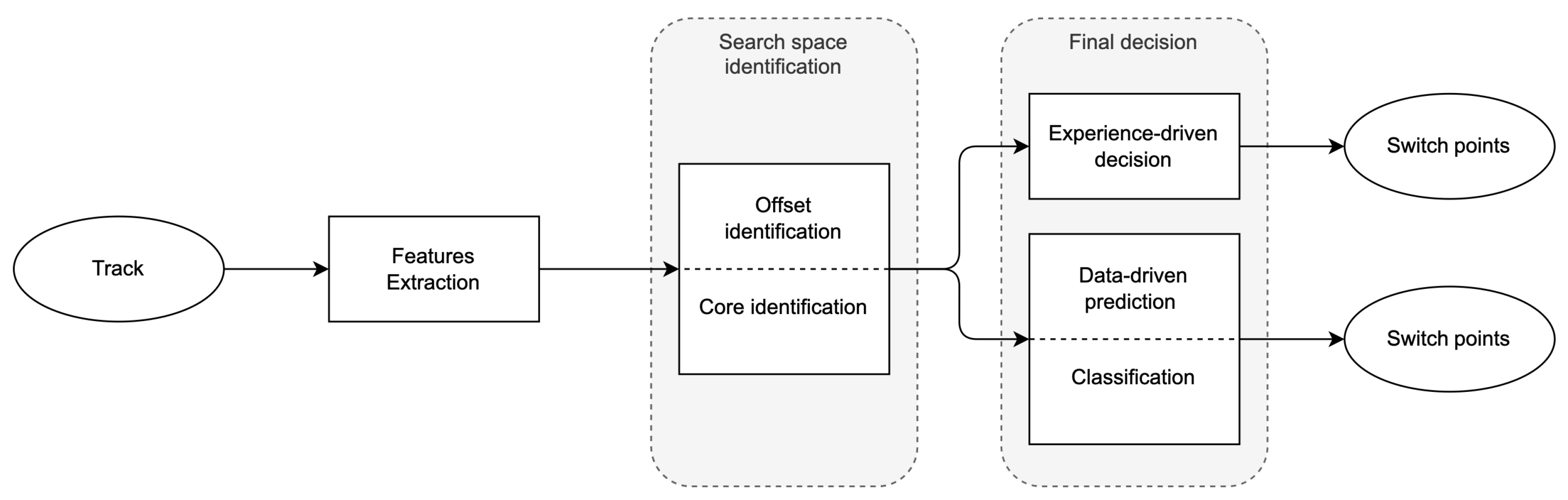
Algorithmically, our approach to SPD consists of two main stages: (1) the identification of a “search space”; that is, a set of candidate positions in the track that are potential switch points, and (2) the final decision of which of the candidates are to be marked as a switch point. For the second stage, we explore one method based on knowledge and intuition (experience-driven) and four methods based on statistics (data-driven). Both stages build on sub-stages, as illustrated in Figure 1, and rely on features extracted from the track.
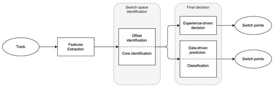
Figure 1.
Algorithmic workflow for both the data- and the experience-driven methods introduced in this article.
3.1. Search Space Identification
As a first step toward the identification of switch points, we construct a search space; that is, a collection of candidate positions that will later undergo a decision process through which they will be either discarded or labeled as switch points. To facilitate this decision process, we want the search space to be as small as possible, but sufficiently large so that good candidates are not prematurely excluded. In the construction of the search space, we leverage two characteristics of EDM tracks: (1) their regularity and (2) their predictability.
3.1.1. Regularity
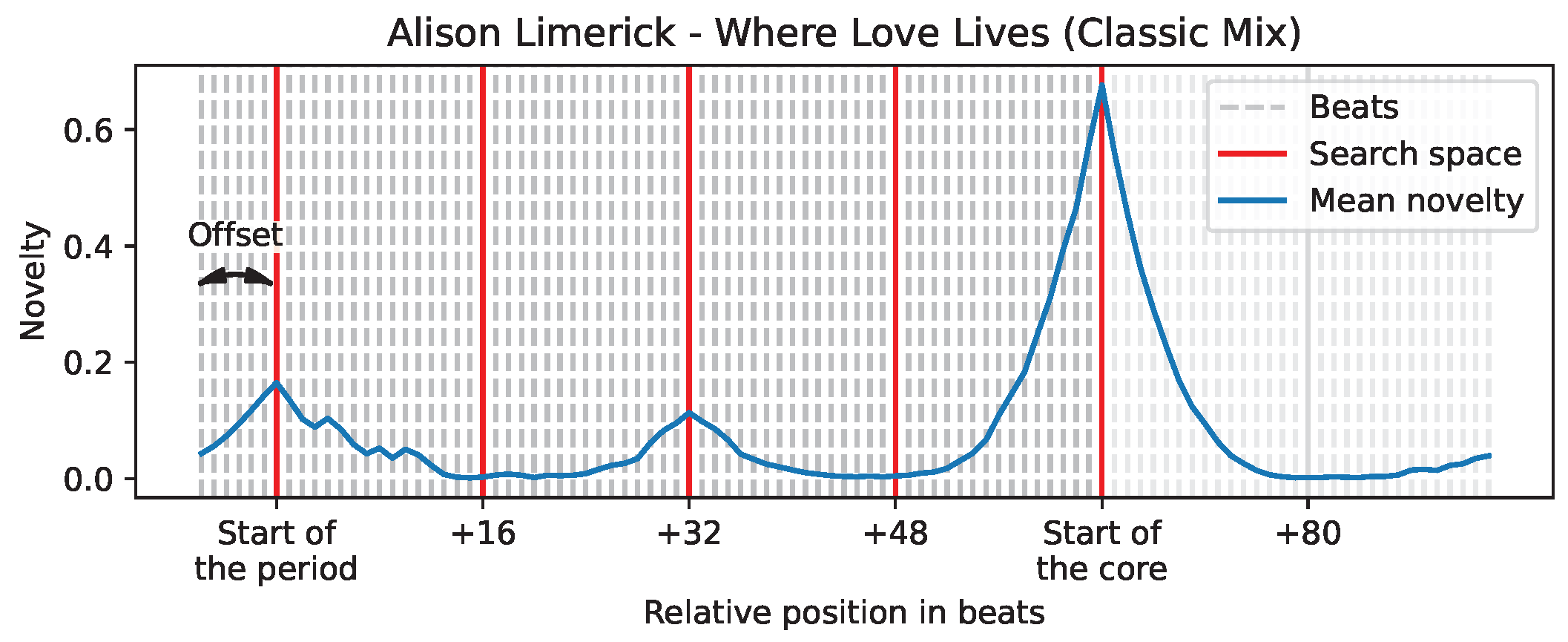
EDM tracks are invariably in 4/4 (i.e., all bars are composed of four beats), and their structure is most often composed of repetitions of four-bar musical periods. As a result, nearly all the segment boundaries—and therefore switch points—are spaced out by a multiple of 16 beats. The four-bar musical period is what professional DJing software typically use to segment bars into groups (e.g., “Traktor pro 3” by Native Instruments). Since the first detected beat in a track need not be the first beat of a bar, and the first bar of a track need not be the first bar of a period, the offset (in beats) to the start of a period has to be identified. Given a four-bar period and the list of beats as potential starting positions, there are 16 possibilities (16 beats)—i.e., an offset of 0–15 beats—to identify the start of the period. One has to choose which of the 16 offsets yields the grid that is more likely to match the structure of the track. To this end, inspired by [16], we rely on novelty: For the 16 different possible offsets, each corresponding to a different grid of points, we compute the average novelty of all its points with CK on multiple features. The grid with the highest value is chosen and constitutes the search space that will then be refined.
3.1.2. Predictability
The structure of EDM tracks is not only regular with respect to its period, but it is also highly predictable with respect to its form. Indeed, all tracks exhibit all or some of three well-defined sections: intro, core, and outro [1]. The intro is stereotypically characterized by a thin texture and several gradual buildups often achieved by layering instruments. It is followed by the core section where the track texture is “full”. The outro is similar to the intro but the texture is progressively “released”. Considering that the core section represents the part the DJ wants to include in the mix, the switch point has to occur before or at the start of this section. To incorporate this insight, we discard from the search space all the positions located after the beginning of the core. The identification of the core section is performed with a heuristic inspired by [16,19]. However, while those authors identify the core as the first segment achieving high energy, we make this rule more restrictive by also requiring the segment to contain a high number of bass drum onsets.
Figure 2 illustrates that the start of the core marks the end of the search space; in the specific case of the track “Where Love Lives” by Alison Limerick, the grid of candidates is now pruned down to only five candidates (depicted with red lines). On average, we observed that the search space consists of 7.4 candidates per track (maximum of 35, minimum of 2).
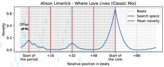
Figure 2.
Visual example of the search space identified.
3.2. Final Decision
After constructing a search space, a decision process follows to select those candidates that should be marked as switch points. DJs’ practice dictates that a newly introduced track should catch the attention of the listener. To incorporate this practice into our process, we aim at keeping only those candidates that mark the boundaries of a salient segment. To this end, we employ the principles of novelty, homogeneity, and repetition.
In the following, we discuss two types of methods to achieve a final decision: experience-driven (or rule-based) and data-driven (or statistics-based). The former consists of implementing the whole decision process according to a pre-determined set of rules, whereas the latter lets some aspects of the decision process emerge from the data without explicitly programming them, but through a training phase (i.e., with machine learning algorithms).
On the one hand, the experience-driven approach is motivated by the fact that DJ practices are well understood and, therefore, we have a clear idea of the musical characteristics required by a position to be considered a switch point. In fact, we are able to code this understanding in a set of verbal rules. On the other hand, implementing those rules as low-level instructions in a programming language is difficult because of the semantic gaps existing among music, verbal, and algorithmic languages. This is illustrated by the difference between the features extracted because they are supposed to be objectively characteristic of a switch point (e.g., signal energy) and how humans effectively perceive those features. For this reason, it is worth contrasting the experience-driven approach with a data-driven approach that, by removing linguistic gaps from the context, may bring an alternative answer to the issue of the relation between the extraction and perception of features for a DJ mix.
We now focus exclusively on the final decision, and outline the implementation of the rules behind the experience-driven approach, and of several statistics-driven methods that draw on the dataset EDM-150.
3.3. Experience-Driven
From the analysis of hundreds of DJ mixes, we concluded that two aspects of a track are especially important for SPD: A change in the energy of the signal—as related to the introduction of the bass register (e.g., with a bass guitar or a change in filtering)—and the entrance of the bass drum. Since these elements are two of the driving forces of EDM and are unquestionably linked to the danceability of a track, the features we are interested in extracting concern mostly their presence. This choice is not only a departure from the methods presented in the related work section, which rely on features associated to timbre and harmony, but is also advantageous for considering features that can be used for the detection of the core section of the track—indeed, we expect that one of the switch points lies exactly at the beginning of the core. However, one notable difference between the two tasks is that for SPD, we rely on the novelty and not on the amplitude of the features, which is instead used for the detection of the core section.
By considering novelty, we can handle two edge cases that would not otherwise be correctly interpreted when considering the amplitude of the features alone. (1) The case of a core section gradually faded in will display high amplitude in the features but not high novelty. As such, it will not lead to the identification of a switch point. This is a desirable outcome as we expect switch points to be positions of salient novelty. (2) The case of a breakdown before the beginning of the core, characterized by a sudden decrease in the amplitude of features and high novelty, will likely be selected as a switch point. This happens because novelty does not depend on the direction of the change, e.g., the progression in the features may be either from high amplitude to low amplitude, or the other way around. This is also a desirable outcome as the start of a breakdown is a valid switch position before the beginning of the core section of the track.
In the following, the detection of the bass register and the bass drum is obtained via the novelty of two different features. Novelty in the bass register is associated with a change in signal energy, which in turn is obtained by calculating the Root Mean Square (RMS) of the signal with Librosa [27]. This quantity is closely related to the perceived loudness of the signal, even though it does not account for the perception of the human ear, which is less sensitive to audio frequencies in the low range. As a result, the RMS of the signal puts a strong emphasis on the bass frequencies. Novelty in the bass drum is associated with the number of onsets in a specific span of time, and its computation relies on automatic drum transcription (ADT) algorithms, as in [28]. The features (i.e., signal energy and onsets numbers) are computed in non-overlapping two-beat windows (between the 1st and the 3rd beat of a 4/4 bar). We choose this window size because we noticed that in many drum patterns, the bass drum emphasizes only the 1st and 3rd beats of a bar (as happens in the standard rock pattern). As observed in other approaches discussed in the related work section, this coarse window size effectively ignores the fine-grained variations in features between beats. A coarser window of one bar (between downbeats) has also been evaluated, but we noticed that the downbeats were not accurately identified in EDM with the software we used from [29]. For each feature, one SSM is built, and CK is applied to compute a novelty with a 32-beat long kernel to compare four-bar periods. Finally, the decision step selects the maximal position in each of the two novelty curves within the search space identified earlier.
3.4. Data-Driven
Whereas the experience-driven approach classifies the positions within a track from their characteristics by using explicit rules, the data-driven approaches perform an initial prediction step in which each candidate position in the search space is assigned a probability score; a score close to 1 indicates that the candidate is likely a switch point, and a score close to 0 indicates that it is not. This prediction is a regression from the characteristics (the features vector) of the candidate position to a probability (a value between 0 and 1); effectively, the prediction is a model trained on known data in the hope that useful patterns for the identification of switch points are learned. The prediction is followed by a classification step to decide, based on the probabilities associated with each candidate, which positions should ultimately be labeled as switch points.
In this section, we discuss four different machine learning methods to train models, and evaluate three of them according to their performance and interpretability. All the methods train a model over multiple features of interest, namely, all those mentioned in the related work section along with those used in ADT. We exploit both the novelty and homogeneity principles (computed with CK), and the repetition principle (computed with SF). For novelty and homogeneity, we employ the same libraries and parameters as those used in the experience-driven approach for energy (RMS), timbre (MFCC), pitch (PCP), and drum onsets. For repetition, we use the same parameters as McFee and Davies did for timbre (MFCC) and pitch (PCP) [13]. To allow models to generalize across tracks, we normalize the values of novelty and repetition so that the value 1 is the maximum within the track.
3.4.1. Deep Learning (DL)
Algorithms based on DL are among the most popular to use to perform music segmentation. Their popularity is due to the expressiveness of their solutions, but these algorithms have two caveats: First, since the models trained with them have many parameters, a lot of training data are required to prevent overfitting; second, because these models are black boxes for which explainable methods still need to be developed in MIR [25] (p. 22), it is difficult to analyze how the output is constructed. This particularly limits their usefulness for the understanding of DJ mixes. Therefore, due to the limited size of our dataset and the inherent lack of explainability of DL-based algorithms, we excluded them from our evaluation.
3.4.2. Linear Classification—Linear Discriminant Analysis (LC-LDA)
In contrast to “linear regression”, a technique to model a continuous variable, “linear classification” predicts a category from a set of observations, and as such, it is better suited for SPD. Multiple algorithms exist for linear classification; examples include the well known logistic regression [30] and linear discriminant analysis. In these algorithms, the model is trained to weigh the input features according to their discriminant capabilities. Then, as in all the other data-driven methods, a classification step follows. Of the two algorithms, we selected the latter as, unlike the former, it has been previously adapted to the task of segment boundary detection [13].
3.4.3. Nonlinear Classification—Decision Tree (NLC-DT)
Nonlinear classification is commonly performed with a decision tree [31]. A tree contains an ensemble of if–else conditions (e.g., ≤ 0.112) predicting the category from the set of observations. These conditions are learned on the training set to separate the data points according to their ground truth category. Furthermore, they are organized in branching paths until sufficient separation is obtained or a maximal depth is reached. This model is easy to interpret but it tends to become overly deep while reaching a good separation of the category. As a result, trees that are too deep usually do not generalize data well (i.e., they overfit), while trees that are too shallow tend to perform poorly (i.e., they underfit). This issue can be solved by training an ensemble of trees.
3.4.4. Nonlinear Classification—Gradient Boosting Decision Trees (NLC-GBDTs)
An alternative solution to obtain better performance than a single decision tree is to employ an ensemble of simple (shallow) trees. This technique is known as “ensemble learning” and is usually implemented in one of two ways: either by “bagging” (as applied by the random forest algorithm) to train trees on different subsets of the data in parallel, or “boosting” (as applied by the GBDT algorithm) to train trees in sequence, where each subsequent tree attempts to correct the errors of the previous one. Of the two techniques, we employ the latter because it achieved better precision with EDM-150 in preliminary tests, as well as being more documented, which helps in its interpretability.
4. Evaluation
An evaluation of the performance of the different computational methods follows.
4.1. Evaluation Metrics
Since SPD plays a central role in the creation of an automatic DJ, we put the emphasis on the precision of each method; that is, the ratio between the number of points estimated by the method that coincide with a human annotation (True Positive) over the total number of estimations returned by the method (i.e., True Positives and False Positives):
In this formula, an estimation is counted as a true positive if it lies within a 0.1 s window around an annotation (for more details, see mir_eval [32]). Precision is computed per track; a score of zero indicates that for the current track, the method produced no correct estimation, or no estimation at all. This effectively penalizes models that are not able to return at least one position per track since it makes those tracks unusable. The precision for a set of tracks is the average of the precision for each separate track; this metric is known as “mean precision”:
The subscript i refers to the i-th track, while n is the total number of tracks (in the test set). and denote the number of True Positive and False Positive estimations in track i, respectively.
In addition to precision, it is common practice to evaluate methods according to their recall, which is the ratio between the number of estimations that coincide with an annotation (True Positive) and the total number of annotations (True Positive and False Negative). We argue that in the context of automatic mixing, recall is not as important as precision; that is, for an algorithm to be adequate, it is important to identify at least one viable switch point as opposed to all the possible ones. In general, the higher the recall (i.e., the more true positives for one given track), the more choices exist to create a transition. However, it is undesirable for a method to have a high recall if this comes at the cost of more false positive estimations. For these reasons, we consider mean precision as the most informative evaluation metric, and we provide the mean recall only as a complementary source of information.
Our evaluation of the final decision (see Section 3 Methods) is conducted in isolation from the identification of the search space. This choice effectively eliminates the impact of errors that could occur in the identification of the offset and the core. In practice, the methods rely on an oracle that provides a search space which consists of manually annotated period boundaries from the start of the tracks until their core. The combined search space of the 150 tracks contains a total of 1948 candidate positions. Of these, 589 coincide with annotations.
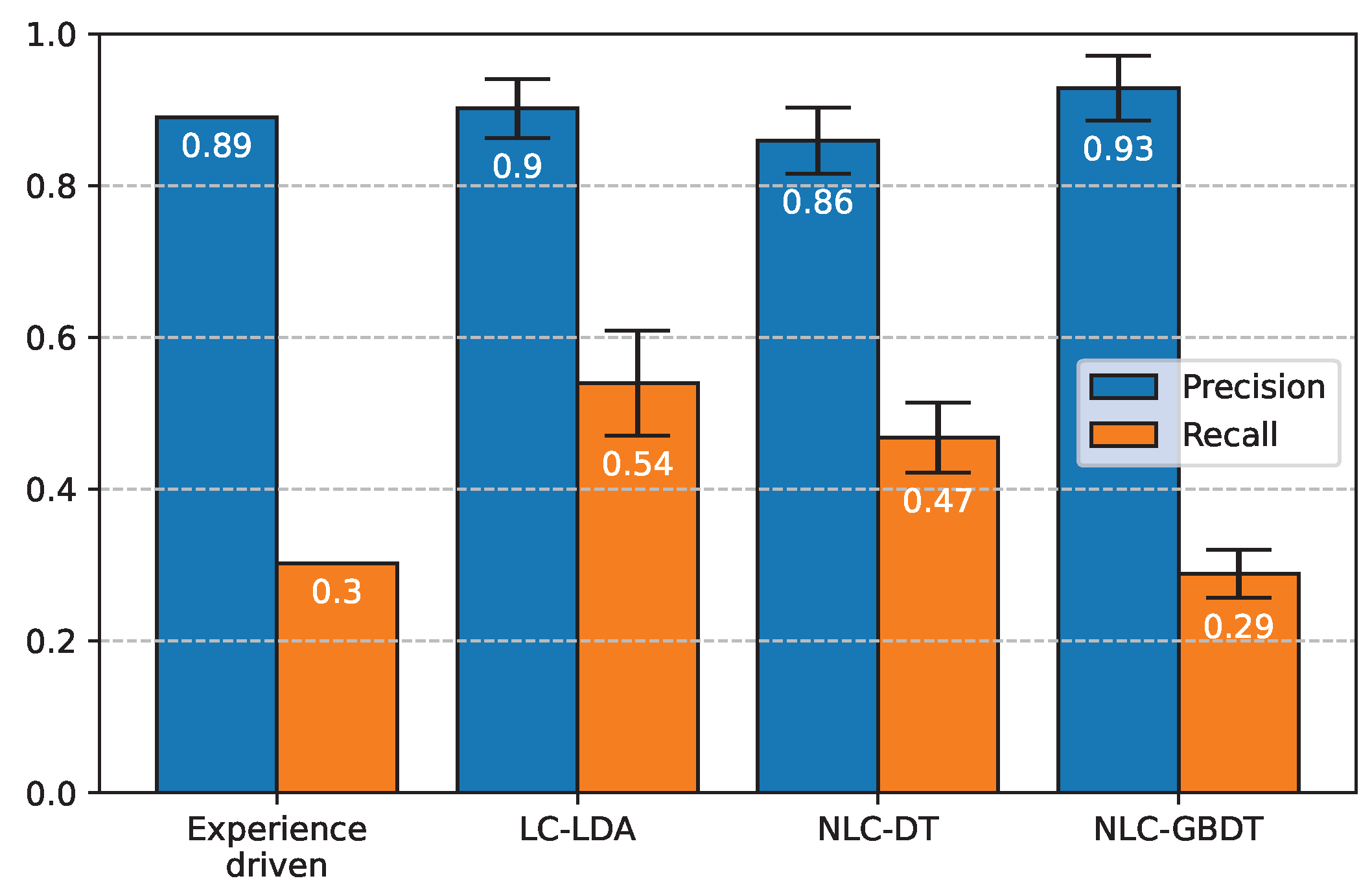
In the evaluation of the data-driven methods, we employed nested cross-validation with a 5-fold split of EDM-150 for the outer loop, and 4-fold split for the inner loop [33]. In the inner loop, the best hyper-parameters (HPs) are identified on a series of train and validation set splits. In the outer loop, the model performance (with the HPs identified) is evaluated on a series of (outer) train and test set splits. By doing the search of HPs in the inner loop, we ensure that the choice of the HPs does not overfit the test sets. By repeating the evaluation on five different test splits with the outer loop, we estimate the generalization capabilities of the methods and report the average score. For the evaluation of the experience-driven method, instead, we performed the evaluation only once on the whole dataset. Figure 3 presents the mean precision and the mean recall for all the methods; a commentary is provided in the following subsections, whereas a separate comparison that includes three baseline methods—“All periods”, “Mixed in Keys”, and “DnB-autoDJ”—appears in [2].
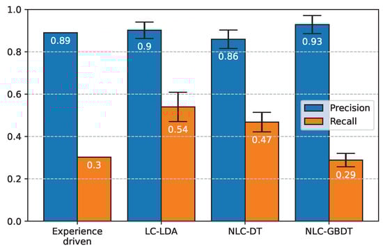
Figure 3.
Quantitative evaluation: Mean precision and mean recall on the EDM-150 dataset. The reported values are the average of the five test splits and the error bars represent the standard deviation. For the experience-driven model, instead, the evaluation is performed only once on the whole dataset.
While nested cross-validation is used to evaluate the generalization capabilities of a method, it does not provide one final trained model. To train such a model, we performed another HP search and training with standard cross-validation on the whole EDM-150, thus effectively reproducing the inner loop of the nested cross-validation but on the whole dataset. This final model is not evaluated (as no data were saved for testing) but can be interpreted with higher confidence as it was trained with more data (compared to the five models in the outer loop of the nested cross-validation).
4.2. Experience-Driven Approach
As shown in Figure 3, this approach achieves 89% precision on EDM-150, on par with the data-driven methods; however, in contrast to those methods, the experience-driven approach accesses only two features and is entirely dataset oblivious (no training or tuning was performed with EDM-150 or any other dataset). Although there are discrepancies between the perception of the features and their computational counterparts (that is, what we extract algorithmically is not necessarily close to what we hear) and that our analysis pertains only to the introduction of a track (not beyond the core), the achieved high precision is the confirmation that our understanding of EDM and the concept of switch point is on point. Since our implementation returns at most two switch points per track (often only one), it should not come as a surprise that the recall is quite low (30%). A posteriori, the results can be further explained by observing that the two features used by the method have the highest correlation with the annotations in EDM-150, and are also highly correlated to one another (i.e., when the bass drum is introduced in the track, there is a substantial change in energy).
4.3. LC-LDA
The mean precision of LC-LDA, 90%, is equivalent to that of the experience-driven approach; this is, however, achieved by operating on many more features. This, in turn, results in a recall of 54%, which is the highest of all the methods considered.
To analyze the patterns used for the classification, we interpret the coefficients learned by the model as shown in Figure 4. The coefficients are interpreted according to their amplitude, which represents the degree of influence of each feature on the estimation of switch points. We can see that, according to LC-LDA, every feature is contributing positively to the construction of a switch point, but, surprisingly enough, the bass drum has one of the lowest contributions among all the features, something that contradicts our intuition behind the experience-driven approach. In fact, it happens that the interpretation of the coefficients returned by the linear classification reveals two main problems: First, because the features are highly correlated with one another (e.g., a change in instrumentation will create both novelty in energy and MFCC), the associated coefficients cannot be seen as covariance between features and decisions. Actually, the interpretation of a single weight depends on all the other features [34] (Section 5.2.5). In our case, the bass drum novelty, which is positively correlated to the perception of a switch point, might have a small coefficient because of the effect of the other correlated features. Second, the performance and interpretability of linear classifications suffer when nonlinearity is present in the relations of the data (e.g., bass drum novelty may not be linearly correlated to the perception of a switch point if the timbral characteristics of the bass drum are altered with a filter). When a situation of this sort occurs, the coefficients learned by the linear classifier are not selecting features for their true association with the dependent variable but for the cancellation effect [35] (p. 57). Because LC-LDA does not perform properly when the features are correlated and nonlinear, we experimented with nonlinear classifiers.
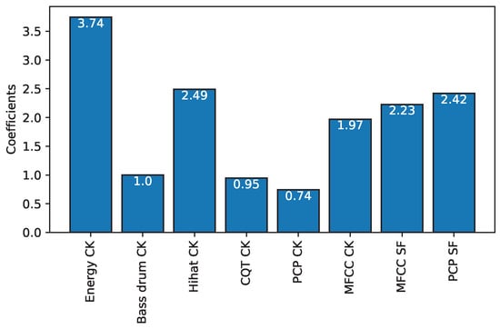
Figure 4.
Coefficients learned by LC-LDA.
4.4. NLC-DT
This approach, although simple, achieves a precision (86%) close to that of the previous two methods. The learned decision rules of this model can be visualized as shown in Figure 5. This method happens to focus exactly on the same two features as the experience-driven approach does (Energy CK, Bass drum CK). Its recall is moderately lower than the LC-LDA’s recall but still higher than the recall of the experience-driven approach.
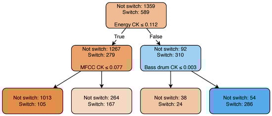
Figure 5.
Decision tree trained on the whole EDM-150. The root node represents the initial distribution of the ground truth labels. Traversing down the tree, the candidates are divided according to the learned decision rules toward the child nodes until reaching the leaves of the tree.
In other words, this method exhibits a behavior close to that of the experience-driven method, but it is less selective. In fact, it selects not only the highest value of each feature (as the experience-driven method does), and it also sets more permeable thresholds on each feature as learned from the database. Furthermore, the features are considered in combination (logical AND) instead of independently from one another (logical OR), as happens with the experience-driven method. As a consequence, the recall for NLC-DT is higher than that of the experience-driven approach.
Figure 5 shows that a third feature, MFCC novelty, is also used. However, MFCC does not manage to further split the data in such a way that one group contains more positive labels than negative ones. This is visible in the decision path of the tree being very short, with only a depth of two. The depth of the decision tree is an HP fitted on the validation data to offer the best compromise between a model too deep or too shallow.
4.5. NLC-GBDT
This method achieves the highest precision (93%) among all methods considered in this study (by contrast, its recall is rather low, 29%). We attribute these results to the fact that this method uses a threshold as a decision rule to select what features are relevant in SPD. The threshold is learned to maximize the mean precision on the validation data, and a very high value is selected so that only one position (the one with the highest probability) is returned for each track.
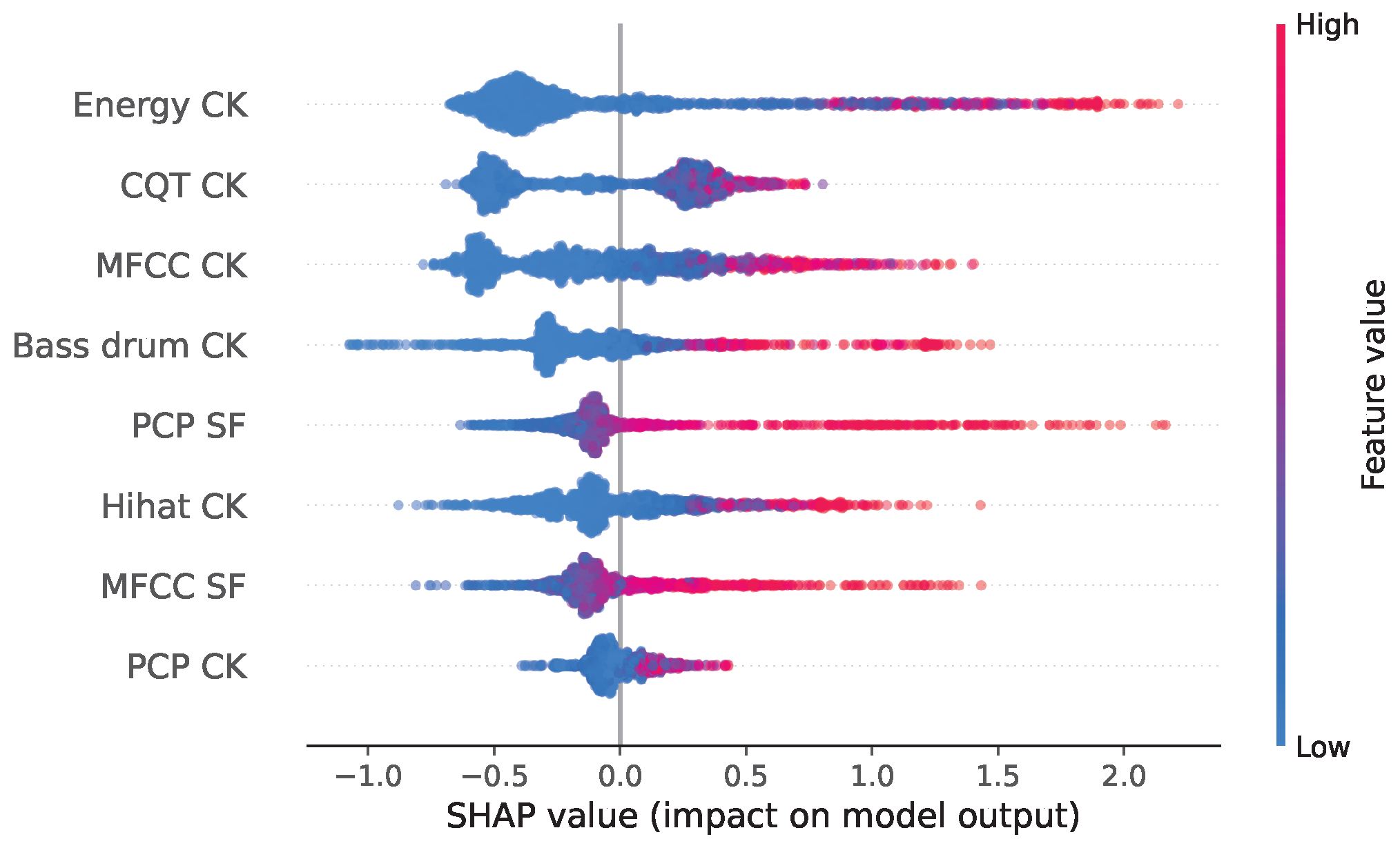
The interpretation of the model is in itself a challenge, as too many trees are generated. Instead, we employ treeExplainer [35], a Python 3 library to estimate SHAP (SHapley Additive exPlanations) values for tree models and ensembles of trees. These values measure the contribution of each feature to the prediction of the model for each sample of the training data. Then, by combining all the local SHAP values, the global explanation of the model is computed and represented with a summary plot, as shown in Figure 6. This global explanation represents the magnitude, prevalence, and direction of the effect for each feature. This plot is comparable to the features’ coefficients learned by the linear classifier, but it singles out the contribution of each feature between the prevalence (number of samples) and magnitude (SHAP value) of its effect. In this plot, each feature is represented on a different row, ordered from top to bottom according to their importance (average influence over every sample). Each dot represents a sample, its color corresponds to the value of the feature for this observation, and its horizontal position represents the SHAP value—the effect that the feature has on the prediction for that sample (i.e., how much the feature changes the output probability of the model). Dots with identical SHAP values are stacked to display the distribution of the effects of the features.
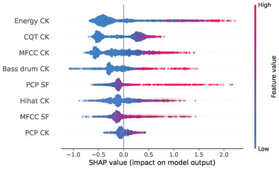
Figure 6.
SHAP summary plot from the Boosting trees model.
On the one hand, for the most part, the summary plot confirms our intuition about the relevance of some features for SPD described in Section 2.2. Specifically, novelty in energy (energy CK), in harmony (CQT CK), and in timbre (MFCC CK) have the strongest effects in this model, whereas novelty in PCP (PCP CK), and repetition of MFCC (MFCC SF) are the least influential features—confirming that pitch distribution is not homogeneous in a segment and that timbre does not display a highly repetitive behavior. On the other hand, the bass drum novelty (Bass drum CK) has a moderate effect, lower than our expectation. While this is not a conclusive explanation, we identify two possible reasons for the limited importance of this feature. First, bass drum novelty is heavily correlated to energy novelty. Since the model will use both features to capture the same effect, the influence of each one on the final decision is smaller than if only one feature were provided. Second, we note that the bass drum onsets are not accurately estimated, see score for “BD” [28] (p. 6), thus adding noise to the feature and reducing its influence.
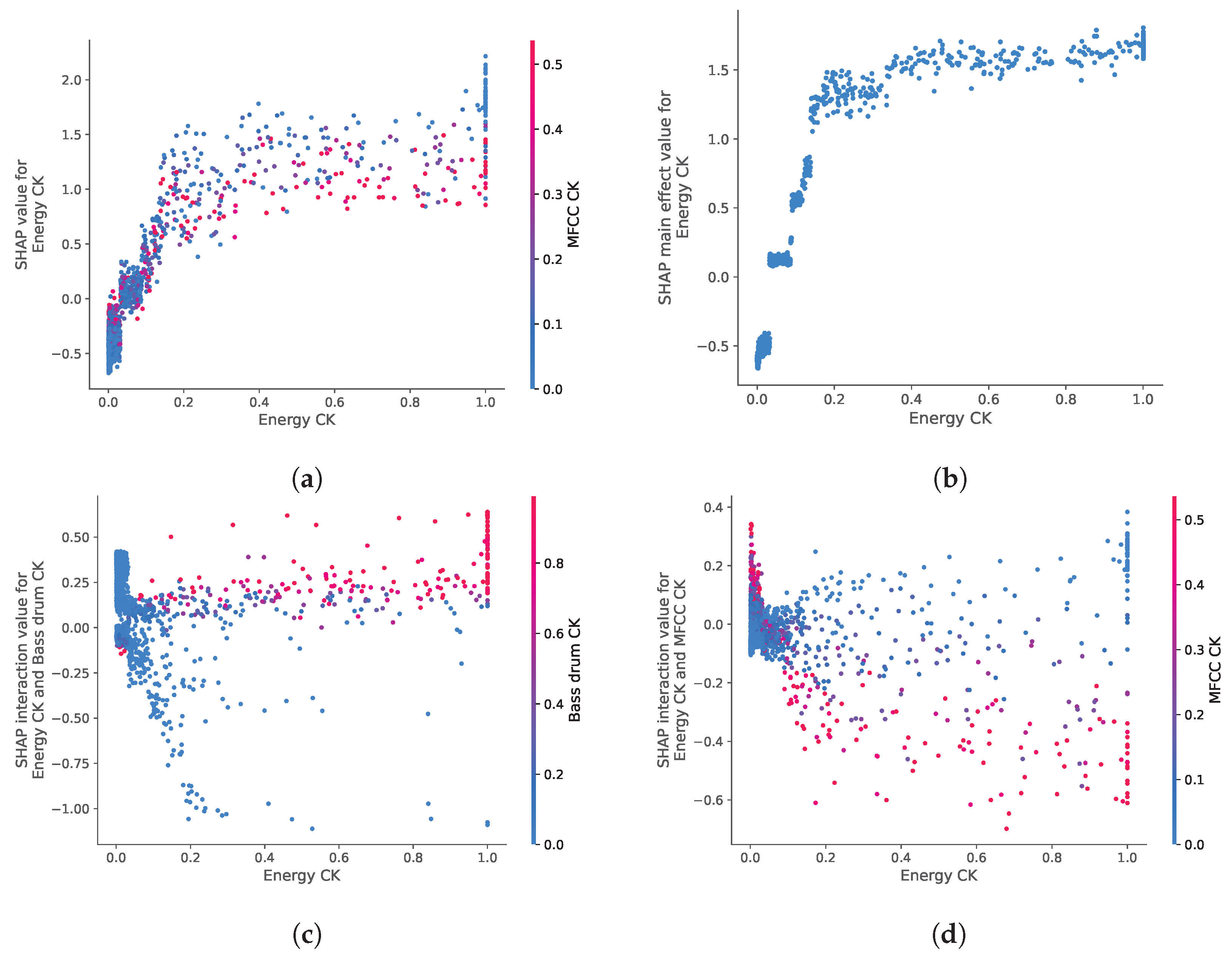
In the summary plot, one can notice samples with the same feature value (color) but different SHAP values (X-position), an effect due to the interactions between features. Such a variation can be shown in a so-called dependence plot, as represented in Figure 7a for the energy novelty. This plot illustrates that when the value of the feature increases, the probability that the position is a switch point increases logarithmically with a wide variance (vertical dispersion) due to the interaction with other features. This variance is explained, at least partially, by the interaction with timbre novelty, whose value is represented by the color of the dots (Figure 7a). In this case, while timbre novelty is the feature with the highest interaction with energy novelty, the overlap of points with different values (color) makes it difficult to characterize its effect.
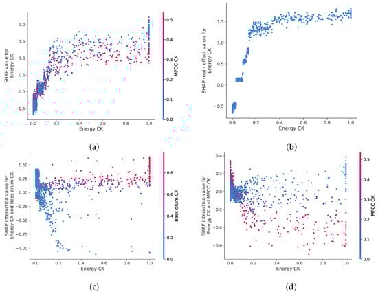
Figure 7.
SHAP dependence and interaction plots for energy novelty: (a) SHAP dependence plot: log relative probability to detect a switch point depending on energy novelty. The spread of the values is mainly due to interaction with timbre novelty. (b) Main effect of energy novelty, without the interaction effect of the other features. The interaction effects of energy novelty with bass drum novelty or timbre novelty are represented in (c) and (d), respectively.
Even though the interaction between the features can be sometimes deduced by the spread of the effect in the dependence plots, it is nonetheless difficult to dissociate the main effect of a feature from the interaction it has with other features. TreeExplainer proposes to use a SHAP interaction plot precisely to separate the effect of a feature (Figure 7a) into the main effect (Figure 7b) and the interaction with the other features (e.g., Figure 7c or Figure 7d). Specifically, the interaction between energy novelty and bass drum novelty (Figure 7c) shows that the model favors a change in energy when there is, at the same time, a change in the bass drum (red-colored dots in the top right region of the plot, i.e., energy novelty and bass drum novelty ). Conversely, the interaction between energy novelty and timbre novelty (Figure 7d) highlights that points with novelty in energy are favored by the model when they display novelty in timbre (blue-colored dots). This is counter-intuitive since both features are desirable for SPD. An inspection of those positions revealed that while high values in both features mainly detect a change in the low-frequency range (e.g., the addition of a bass line, or the release of a high-pass filter), positions of high energy novelty and low timbre novelty mainly detect changes occurring exclusively to the drum instruments (i.e., the addition of bass drum, hi-hat, and snare drum). Thus, according to the model, a change in energy caused by the drum instruments seems relatively more favorable for SPD.
5. Conclusions
Our research focused on the identification of switch points, a specific set of positions within a musical track that are conducive to transitions in a DJ mix. Our study aimed at (1) the evaluation of several methods to perform this identification automatically, either based on knowledge and intuition, or statistics, and (2) the interpretation of these methods to determine the features that have the highest impact in the decision process leading to SPD. Similar studies were conducted by Nieto et al. [14], but those were concerned with the more general task of structure analysis, whereas we focused specifically on SPD. To perform this study, we curated EDM-150, a dataset annotated by experts and currently the only dataset that contains precise and exhaustive locations of switch points in EDM tracks. Our results show that changes in energy, harmony, and timbre are the most effective features for SPD. Changes in the density of drum onsets also play a role but to a lesser extent. We also observed that the features interact with each other and are not linearly connected to the identification of the points.
Despite these promising results, our study has some limitations: in any methods based on expert knowledge, the formalization and implementation of human decisions follow a heuristic process of trial and error whose subjectivity yields good but not necessarily optimal outcomes; instead, in the case of methods based on a data-driven approach, limitations may derive from the size and quality of the training dataset or by the statistical model itself, if this is not suitable for the task. In the future, should a larger dataset become available, it would be interesting to see how the accuracy of the models would be affected. It would also be interesting to validate our findings by testing a variety of tracks that either are more recent than those used in the training dataset or cover genres that were underrepresented or not represented at all. Additionally, we plan to analyze the accuracy of the drum transcription feature and determine whether the errors in the onsets detected hinder the capability to identify switch points.
Author Contributions
Conceptualization, M.Z., M.A. and P.B.; methodology, M.Z., M.A. and P.B.; software, M.Z.; validation, M.Z.; formal analysis, M.Z. and P.B.; investigation, M.Z.; data curation, M.Z., M.A. and P.B.; writing—original draft preparation, M.Z.; writing—review and editing, M.A. and P.B.; visualization, M.Z.; supervision, M.A. and P.B.; funding acquisition, P.B. All authors have read and agreed to the published version of the manuscript.
Funding
This research was supported by the eSSENCE Programme under the Swedish Government’s Strategic Research Initiative.
Data Availability Statement
The code used in this work is available here: https://github.com/MZehren/Automix (accessed on 24 September 2024). The dataset used in this work is available at this location: https://github.com/MZehren/M-DJCUE (accessed on 24 September 2024).
Conflicts of Interest
The authors declare no conflicts of interest.
References
- Butler, M.J. Unlocking the Groove: Rhythm, Meter, and Musical Design in Electronic Dance Music. Ph.D. Thesis, Indiana University, Bloomington, IN, USA, 2003. [Google Scholar]
- Zehren, M.; Alunno, M.; Bientinesi, P. Automatic Detection of Cue Points for the Emulation of DJ Mixing. Comput. Music. J. 2022, 46, 16. [Google Scholar] [CrossRef]
- Kell, T.; Tzanetakis, G. Empirical Analysis of Track Selection and Ordering in Electronic Dance Music using Audio Feature Extraction. In Proceedings of the 14th International Society for Music Information Retrieval Conference, ISMIR 2013, Curitiba, Brazil, 4–8 November 2013; pp. 505–510. [Google Scholar]
- Kim, T.; Choi, M.; Sacks, E.; Yang, Y.H.; Nam, J. A Computational Analysis of Real-World DJ Mixes using Mix-To-Track Subsequence Alignment. In Proceedings of the 21st International Society for Music Information Retrieval Conference, Virtual, 11–16 October 2020; pp. 764–770. [Google Scholar]
- Bittner, R.M.; Gu, M.; Hernandez, G.; Humphrey, E.J.; Jehan, T.; McCurry, P.H.; Montecchio, N. Automatic Playlist Sequencing and Transitions. In Proceedings of the 18th International Society for Music Information Retrieval Conference, Suzhou, China, 23–27 October 2017; pp. 472–478. [Google Scholar]
- Paulus, J.; Klapuri, A. Audio-based music structure analysis. In Proceedings of the 11th International Society for Music Information Retrieval, Utrecht, The Netherlands, 9–13 August 2010; pp. 625–636. [Google Scholar]
- Wang, J.C.; Smith, J.B.L.; Lu, W.T.; Song, X. Supervised Metric Learning for Music Structure Features. In Proceedings of the 22th International Society for Music Information Retrieval Conference, Online, 7–12 November 2021; pp. 730–737. [Google Scholar]
- Foote, J. Automatic audio segmentation using a measure of audio novelty. In Proceedings of the IEEE International Conference on Multimedia and Expo, New York, NY, USA, 30 July–2 August 2000; Volume 1, pp. 452–455. [Google Scholar] [CrossRef]
- Serra, J.; Muller, M.; Grosche, P.; Arcos, J.L. Unsupervised Music Structure Annotation by Time Series Structure Features and Segment Similarity. IEEE Trans. Multimed. 2014, 16, 1229–1240. [Google Scholar] [CrossRef]
- Kaiser, F.; Peeters, G. A simple fusion method of state and sequence segmentation for music structure discovery. In Proceedings of the 14th International Society for Music Information Retrieval Conference, Curitiba, Brazil, 4–8 November 2013. [Google Scholar]
- McFee, B.; Ellis, D.P.W. Analyzing song structure with spectral clustering. In Proceedings of the 15th International Society for Music Information Retrieval Conference, Taipei, Taiwan, 27–31 October 2014; pp. 405–410. [Google Scholar]
- Nieto, O.; Mysore, G.J.; Wang, C.i.; Smith, J.B.L.; Schlüter, J.; Grill, T.; McFee, B. Audio-Based Music Structure Analysis: Current Trends, Open Challenges, and Applications. Trans. Int. Soc. Music Inf. Retr. 2020, 3, 246–263. [Google Scholar] [CrossRef]
- McFee, B.; Ellis, D.P. Learning to segment songs with ordinal linear discriminant analysis. In Proceedings of the IEEE International Conference on Acoustics, Speech and Signal Processing (ICASSP), Florence, Italy, 4–9 May 2014; pp. 5197–5201. [Google Scholar] [CrossRef]
- Nieto, O.; Bello, J.P. Systematic exploration of computational music structure research. In Proceedings of the 17th International Society for Music Information Retrieval Conference, New York City, NY, USA, 7–11 August 2016; pp. 547–553. [Google Scholar]
- Rocha, B.; Bogaards, N.; Honingh, A. Segmentation and Timbre Similarity in Electronic Dance Music. In Proceedings of the 10th Sound and Music Computing Conference, Stockholm, Sweden, 30 July–2 August 2013; pp. 754–761. [Google Scholar]
- Vande Veire, L.; De Bie, T. From raw audio to a seamless mix: Creating an automated DJ system for Drum and Bass. EURASIP J. Audio Speech Music Process. 2018, 2018, 13. [Google Scholar] [CrossRef]
- Davies, M.E.P.; Hamel, P.; Yoshii, K.; Goto, M. AutoMashUpper: Automatic Creation of Multi-Song Music Mashups. IEEE/ACM Trans. Audio Speech Lang. Process. 2014, 22, 1726–1737. [Google Scholar] [CrossRef]
- Yadati, K.; Larson, M.; Liem, C.C.S.; Hanjalic, A. Detecting Drops in Electronic Dance Music: Content based approaches to a socially significant music event. In Proceedings of the 15th International Society for Music Information Retrieval Conference, Taipei, Taiwan, 27–31 October 2014; pp. 143–148. [Google Scholar]
- Schwarz, D.; Schindler, D.; Spadavecchia, S. A Heuristic Algorithm for DJ Cue Point Estimation. In Proceedings of the Sound and Music Computing (SMC), Limassol, Cyprus, 4–7 July 2018. [Google Scholar]
- McCallum, M.C. Unsupervised Learning of Deep Features for Music Segmentation. In Proceedings of the ICASSP 2019—2019 IEEE International Conference on Acoustics, Speech and Signal Processing (ICASSP), Brighton, UK, 12–17 May 2019. [Google Scholar] [CrossRef]
- Salamon, J.; Nieto, O.; Bryan, N.J. Deep Embeddings and Section Fusion Improve Music Segmentation. In Proceedings of the 22th International Society for Music Information Retrieval Conference, Online, 7–12 November 2021; p. 8. [Google Scholar]
- Ullrich, K.; Schlüter, J.; Grill, T. Boundary Detection in Music Structure Analysis using Convolutional Neural Networks. In Proceedings of the 15th International Society for Music Information Retrieval Conference, Taipei, Taiwan, 27–31 October 2014. [Google Scholar]
- Grill, T.; Schluter, J. Music boundary detection using neural networks on spectrograms and self-similarity lag matrices. In Proceedings of the 2015 23rd European Signal Processing Conference (EUSIPCO), Nice, France, 31 August–4 September 2015; pp. 1296–1300. [Google Scholar] [CrossRef]
- Wang, J.C.; Hung, Y.N.; Smith, J.B.L. To Catch A Chorus, Verse, Intro, or Anything Else: Analyzing a Song with Structural Functions. In Proceedings of the ICASSP 2022—2022 IEEE International Conference on Acoustics, Speech and Signal Processing (ICASSP), Singapore, 23–27 May 2022; pp. 416–420. [Google Scholar] [CrossRef]
- Peeters, G. The Deep Learning Revolution in MIR: The Pros and Cons, the Needs and the Challenges. In Perception, Representations, Image, Sound, Music; Kronland-Martinet, R., Ystad, S., Aramaki, M., Eds.; Series Title: Lecture Notes in Computer Science; Springer International Publishing: Cham, Switzerland, 2021; Volume 12631, pp. 3–30. [Google Scholar] [CrossRef]
- Schwarz, D.; Fourer, D. Methods and Datasets for DJ-Mix Reverse Engineering. In Perception, Representations, Image, Sound, Music; Kronland-Martinet, R., Ystad, S., Aramaki, M., Eds.; Springer: Cham, Switzerland, 2021; pp. 31–47. [Google Scholar]
- McFee, B.; Raffel, C.; Liang, D.; Ellis, D.; McVicar, M.; Battenberg, E.; Nieto, O. librosa: Audio and Music Signal Analysis in Python. In Proceedings of the SciPy, Austin, TX, USA, 6–12 July 2015; pp. 18–24. [Google Scholar] [CrossRef]
- Vogl, R.; Widmer, G.; Knees, P. Towards multi-instrument drum transcription. In Proceedings of the 21th International Conference on Digital Audio Effects (DAFx-18), Aveiro, Portugal, 4–8 September 2018. [Google Scholar]
- Böck, S.; Krebs, F.; Widmer, G. Joint Beat and Downbeat Tracking with Recurrent Neural Networks. In Proceedings of the 17th International Society for Music Information Retrieval Conference, New York City, NY, USA, 7–11 August 2016; pp. 255–261. [Google Scholar]
- Hosmer, D.W.; Lemeshow, S. Applied Logistic Regression, 2nd ed.; Wiley Series in Probability and Statistics; Wiley: New York, NY, USA, 2000. [Google Scholar]
- Hastie, T.; Tibshirani, R.; Friedman, J.H. The Elements of Statistical Learning: Data Mining, Inference, and Prediction, 2nd ed.; Springer Series in Statistics; Springer: New York, NY, USA, 2009. [Google Scholar]
- Raffel, C.; McFee, B.; Humphrey, E.J.; Salamon, J.; Nieto, O.; Liang, D.; Ellis, D.P.W. mir_eval: A transparent implementation of common MIR metrics. In Proceedings of the 15th International Society for Music Information Retrieval Conference (ISMIR), Taipei, Taiwan, 27–31 October 2014; pp. 367–372. [Google Scholar]
- Cawley, G.C.; Talbot, N.L.C. On Over-fitting in Model Selection and Subsequent Selection Bias in Performance Evaluation. J. Mach. Learn. Res. 2010, 11, 2079–2107. [Google Scholar]
- Molnar, C. Interpretable Machine Learning: A Guide for Making Black Box Models Explainable, 2nd ed.; Independently Published; 2022; Available online: https://christophm.github.io/interpretable-ml-book/index.html (accessed on 24 September 2024).
- Lundberg, S.M.; Erion, G.; Chen, H.; DeGrave, A.; Prutkin, J.M.; Nair, B.; Katz, R.; Himmelfarb, J.; Bansal, N.; Lee, S.I. From local explanations to global understanding with explainable AI for trees. Nat. Mach. Intell. 2020, 2, 56–67. [Google Scholar] [CrossRef] [PubMed]


Disclaimer/Publisher’s Note: The statements, opinions and data contained in all publications are solely those of the individual author(s) and contributor(s) and not of MDPI and/or the editor(s). MDPI and/or the editor(s) disclaim responsibility for any injury to people or property resulting from any ideas, methods, instructions or products referred to in the content. |
© 2024 by the authors. Licensee MDPI, Basel, Switzerland. This article is an open access article distributed under the terms and conditions of the Creative Commons Attribution (CC BY) license (https://creativecommons.org/licenses/by/4.0/).