Abstract
Cruising-for-parking in an urban area is a time-consuming and frustrating activity. We present four machine learning-based models to predict the parking availability of street segments in an urban area on a three-level scale, which navigator and smart-parking apps can exploit to ease and reduce the cruising phase. The models were trained with data generated by a cruising-for-parking simulator that we developed, replicating four parking behavior types (workers, residents, buyers, and visitors). The generated data is comparable to that collectible with smartphones’ sensors. We simulated 40 users moving for 200 weeks in the city area of San Giovanni in Rome. We collected information about users’ parking, unparking, and cruising actions over considered road segments at different time slots. Once a significant amount of trips were collected, we extracted ten features for each road segment at a given time slot. With the obtained dataset, which contained 761 samples, we trained and compared four supervised machine learning models that receive the history of a segment and, in return, classify the Parking Availability Level of the segment as Green, Yellow or Red. The four models were further evaluated in a different city area, San Lorenzo, and obtained very accurate results. We can predict parking availability with an accuracy above 97% for all the street segments where we collected 30 or more user actions, confirming the robustness of the simulator in generating synthetic cruising-for-parking data and the suitability of designing a Parking Availability Classifier (PAC) based on data collectible by smartphones.
1. Introduction
Cruising for parking is a time-consuming, frustrating activity, and it also has adverse effects on traffic, air pollution, and noise [1]. Knowing where it is more likely to find a free parking spot at a street segment level can help reduce cruising for parking time, thus decreasing fuel consumption, pollution, and local traffic. Artificial Intelligence can empower the user involved in the cruising for parking tasks by predicting on-street parking availability in dense urban areas.
Making such a prediction requires facing the significant problem of collecting data at the area and street levels about parking usage, trips, and traffic flow at different times in the day and over the week. Moreover, collecting data about parking availability can be time and resource-consuming, as it is information that changes over time and requires on-site validation.
In this research paper, we propose four machine learning models to classify the parking availability probability of a given road segment by analyzing contextual data that can be collected inexpensively through smartphones, as they are so widespread and well connected to the internet in urban areas. Our work aims at demonstrating that data collectible by smartphones is suitable to design a Parking Availability Classifier (PAC).
The models estimate the probability of finding a parking spot on a three-level scale. A navigator app can use this estimation to color the street segments of roads in the destination area on its map.
Our challenge was to train and run the models with little data. For this reason, before implementing our system, we conducted a behavioral study with field interviews and created a simulator to generate realistic synthetic data.
We organize the paper as follows. First, we discuss the related literature. Then, in Section 3 and Section 4, we present the Cruising for Parking Simulator (CPS) we developed and explain how we generated synthetic trip data for the data collection phase. In Section 5 and Section 6, we discuss how, once we extracted the relevant features, we trained and compared four machine learning models using the simulated data to classify the street segments. In Section 7 we report on the evaluation of the models to demonstrate their robustness. We could predict parking availability with an accuracy above 97% for all the street segments where we collected 30 or more user actions (e.g., cruising, parking, unparking). In Section 8, we discuss the results obtained, and in Section 9 we illustrate the applicability of our work in smart-parking apps. Finally, in Section 10 we draw the conclusions of our work, and in Section 11 we describe future research goals.
2. Related Work
Detecting and predicting parking occupancy has been one of the most discussed topics in the transportation system literature of the last decade.
Comparing our work with the existing approaches to solve the problem of parking availability prediction is not immediate. Indeed, how the studies collect and model data varies significantly. Moreover, the performance evaluation of individual studies depends on whether they want to predict the availability of individual parking lots, segments, or zones. We aim to predict the 3-level classification (low, medium, high) of the parking availability of road segments for which we have collected enough historical data (at least 30 park, unpark and cruising actions).
To the best of our knowledge, none of the previous studies relied on smartphones’ sensors only to collect data.
2.1. Off-Street vs. On-Street Parking Availability Prediction
First, we must focus on the clear difference between on-street and off-street parking. Off-street parking often takes advantage of Internet-of-Things (IoT) sensor components, making it easier and more accurate to assess the number of vacancies. For example, in [2] prediction is done through cameras to notify when a space becomes free. In [3], they notify the presence of a car in a given space through motion sensors. Ref. [4] predicts availability via roadside parking sensors and machine learning (ML). Ref. [5] uses vehicle- and street-sensors. Finally, Ref. [6] enables tagging parking spots in the city without the need for sensor infrastructure classifying private and public parking spots. We assimilated the probabilistic approach at a street precision level from the research above.
It is more challenging to predict on-street parking as there is usually less information. For example, the study in [7] used in-car dashcams images to collect data on available parking spaces. Some of these studies rely on collecting data on parking spaces within defined areas, including the use of sensors [8]. Other studies are based on datasets made available by the city itself, on which they then apply neural network algorithms to make predictions on parking availability [9]. Finally, others detect the location and type of parking using the driver’s smartphone [10].
2.2. Machine Learning vs. Deep Learning Approaches
In recent years, within a variety of methods, Neural Networks (NN) and Recurrent Neural Networks (RNN) appear to be the most used. In particular, methods that adopt Deep Learning (DL) are receiving growing interest.
We refer to [11] for an extensive review of ML- and DL-based works before 2019 on parking availability prediction. As for the papers following 2019, Table 1 is an extension of a table presented in [11], providing an overview and a comparison of the most recent research works.
Among the most recent works that adopted DL-based methods, Ref. [12] presented a hybrid framework based on both Convolutional Long-Short Term Memory (LSTM) Networks and Dense Convolutional Networks to make short- and long-term predictions on the parking availability zone-wisely. Previously, also Ref. [13] proposed a system to predict the level of parking occupancy on a block-level scale. This work adopted as models Graph Convolutional Neural Networks (CNN) and LSTM and considered multiple data sources, including parking meters transactions and traffic data. Ref. [14] proposed two deep learning approaches to forecast the occupancy of street parking sectors, namely LSTM and Gated Recurring Unit (GRU). Finally, Ref. [15] proposed a parking occupancy detection system based on Deep Extreme Learning Machine (DELM), and they achieved 91.25% of accuracy during testing. All the mentioned works mainly relayed on occupancy sensors data.
However, recent literature also argues that deep learning methods are too complex compared to the results obtained, which are sometimes even worse than those of more straightforward approaches.
For example, Ref. [16] presents a comparative analysis of different ML- and DL-based models to solve the parking availability prediction problem, using data collected from sensors on individual parking lots and external factors, as pedestrian volume and traffic data. The results show that a Random Forest (RF) is the best model for their target. Similarly, Awan et al. compared different models from ML and DL for parking availability prediction in [17]. They analyzed RF, Decision Tree (DT), K-Nearest Neighbor (KNN), Multilayer Perceptron (MLP), and Ensemble Learning over a dataset coming from an IoT sensor network. Their results show that DT and RF outperform the accuracy of every other algorithm they consider. In [18], Paidi et al. compare three different models (LSTM, Seasonal Auto-Regressive Integrated Moving Average with exogenous variables (SARIMAX), and Ensemble-based method, based on DTs and RFs). They address this problem using thermal camera images. The Ensemble-based method and LSTM performed best, with minimal variation. Additionally, [11], after analyzing deep learning approaches, propose a system based on RFs. Finally, random forests were found to be the most suitable model also for the research carried out in [19]. However, in this case the authors did not consider deep learning models, nonetheless comparing different models from linear regression up to ANNs. Even these works relayed mainly on occupancy sensors data.
Ref. [20] is the only other work that relayed, as in our case, on data collected by smartphones. Here, Arora et al. presented two models for parking availability estimation, one based on a single-layer multiclass regression and another based on a feedforward Deep Neural Network (DNN), while the DNN they presented shows better performance in generalization, the accuracy over the same city shows no improvement when using the DNN in place of the regressor. Furthermore, they showed that training both models using data from local cities is far better than trying to generalize between cities.
In our research we used and compared four different ML models to tackle this problem without involving complex techniques like deep neural networks. We are strongly supported in this choice by the cited literature.

Table 1.
Extension of the table presented in [11]; comparison of related works after 2019.
Table 1.
Extension of the table presented in [11]; comparison of related works after 2019.
| Year | Goal | Metric | Performance | Method | Data Sources | |
|---|---|---|---|---|---|---|
| [13] | 2019 | Predict block-level parking occupancy | MAE | 1.69 (30 min in advance) | Graph CNN, LSTM | Multiple data sources, including parking meter transactions, traffic speed data, roadway networks, and weather conditions |
| [20] | 2019 | Estimate the difficulty of parking at a particular time and place | Improvement delta (D), Balanced normalized rewards (BNR) | (Improvement from single-layer model to DNN) D: 0.002 to 0.118, (Improvement from DNN trained on SF and tested on other cities, to DNN trained and tested locally) D: 0.06 to 0.1 | Single-layer multiclass regression ML model, DNN | Smartphone user location data, surveys for ground truth data |
| [15] | 2020 | Parking occupancy detection | Accuracy (%), MSE | (Training) Accuracy: 94.37, MSE: 3.93, (Testing) Accuracy: 91.25, MSE: 1.06 | DEML | Occupancy sensors |
| [11] | 2020 | Predict occupancy rate | MSE, MAE | (For 60 min. ahead, NN) MSE: 7.18, MAE: 1.87 (For 60 min. ahead, RF) MSE: 7.98, MAE: 1.92 | NN, RF | Traffic and parking sensors, forecasting Web Services |
| [14] | 2020 | Generate forecasted information on parking slots availability | RMSE | (Best results obtained over 4 cities compared) GRU: 0.089, LSTM: 0.093 | LSTM, GRU | Under road sensors + exogenous data (hourly weather and calendar effects) |
| [17] | 2020 | Comparative analysis of well-known methods for on-street parking availability prediction (10–20 min time frame) | Precision (%), Recall (%), F1-Score (%), Accuracy (%) | Best model after comparison: DT. (Performance on the most critical scenario: 20-min Prediction Validity, 80% threshold) Precision: 85.42, Recall: 84.13, F1-Score: 84.77, Accuracy: 87.82 | RF, DT, KNN, MLP, Ensemble Learning (EL) combining the other methods | Occupancy sensors (data provided by Santander City) |
| [19] | 2020 | Comparative analysis of well-known methods for on-street parking availability prediction | MAE, RMSE, Coefficient of determination R2 | Best model after comparison: RF. MAE: 2.16, RMSE: 21.65, R2: 0.87 | Dummy regression, Linear Regression, DT, GB, RF, KNN, ANN | Occupancy sensors (data provided by Melbourne City) |
| [12] | 2022 | Short-term (<=30 min) and long-term (>30 min) predictions on vacant parking space availability zone-wisely | RMSE, MAE, MAPE (%) | (60 min. ahead) RMSE: 24.60, MAE: 17.69, MAPE: 7.28, (15 min. ahead) RMSE: 10.68, MAE: 7.69, MAPE: 3.04 | dConvLSTM-DCN | Data provided by Santa Monica Open Data Portal |
| [16] | 2022 | Comparative analysis of well-known methods to analyze the impact of external factors on on-street parking availability prediction (5–10 min time frame) | Accuracy (%), AUC | Best model after comparison: RF. Accuracy: 81, AUC: 0.18 | RF, DT, KNN, Gradient Boosting (GB), Adaptive Boosting, MLP, and linear Support Vector Machine | Occupancy sensors, pedestrian volume, weather, traffic data |
| [18] | 2022 | Provide short-term predictions on parking availability with low volume of data | MAE, RMSE | (Best and worst results for each scenario) Weekend prediction: EL. MAE: 2.13, 2.92, Weekend prediction + visitor trend data: EL. MAE: 1.97, RMSE: 2.63, Weekday prediction: LSTM. MAE: 2.9, RMSE: 3.54, Weekday prediction + visitor trend data: SARIMAX. MAE: 2.86, RMSE: 3.42 | LSTM, SARIMAX, EL combining DTs and RFs | Occupancy data manually extracted by analyzing thermal images + visitor trend data |
| This paper | 2022 | Predict parking availability on street segment level with data collected by smarpthones | Accuracy (%), Precision (%), Recall (%), F1-score (%) on labels 0, 1, and 2 | Best two models after comparison: RF and ANN. Accuracy: 97 (both), Precision: 100, 98, 96 (RF); 96, 98, 96 (ANN); Recall: 94, 95, 100 (RF), 89, 94, 100 (ANN); F1-score: 97, 97, 98 (RF), 92, 96, 98 (ANN) | KNN, GB, RF, ANN | Smartphone data generated with CPS |
2.3. Source of Inspiration
Our primary literature source and inspiration is Arora et al. [20] where the Google researchers present a great variety of features, useful for understanding and finding the different aspects that indicate parking difficulty. Like ours, it is one of the few works assessing the number of parking spaces and what happens during the trip. They accomplished their results on an area precision level. Our main challenge is to bring a more accurate and detailed precision, making our prediction at the street level, with a less populated and diversified dataset than the Google one.
Moreover, Arora et al. deliver some challenges in the first steps of their research regarding people’s subjectivity in response to their data surveys. For this reason, we decided to exploit information only from areas and people we know so that our data would be consistent and not as error-prone as it would be from unknown sources. We put together from Google’s research the various features that we rely on, except for those based on Google’s access to the user’s information. We also relied on a similar approach to the ground truth data, such as surveys. Furthermore, we exploit the prediction output labels from their studies so that the parking availability prediction would give us results as levels, such as easy, medium, and limited. We then converted them into green, yellow, and red to show them on a map.
As mentioned before, our research does not consider information from the vehicle speed and acceleration values, traffic conditions, or real-time data from IoT or other sensor devices. As highlighted by Errousso et al. [19], it is still possible to predict parking occupancy by carrying out different features. In particular, their research analyzes drivers entering a specific area they interact with. They exploit features like occupied places, the number of available places, the oncoming vehicles, and the departing vehicles. The whole dataset gathers around a particular time of the week and a specific time of the day. We assemble from their studies the level and methodologies of data preprocessing to make machine learning work properly. They perform several preprocessing phases, such as removing unnecessary or redundant information, determining the periods they want to examine, and finally calculating the different parameters they need to exploit. They also consider a survival analysis of parking space availability, i.e., the probability, over a priori fixed time interval, that a driver finds occupied a parking spot that should have been free as someone just left. We do not count this feature for our purpose, as our studies refer to a less peculiar and low-level accuracy.
3. Cruising for Parking Simulator
Researchers use simulators of various types, as these allow real-world situations to be observed and replicated in a controlled experimental world.
The proposed simulator can build realistic car trips in actual city maps from the point of departure to a wished destination by focusing on the cruising-for-parking phase of the trip. The system assumes that every trip ends with an on-street parking search. Its main goal is to collect large amounts of data about cruising for parking phases and on-street parking availability.
A simulation session can include multiple car trips carried out by different users over a specified time range. Each simulation collects information about the complete path of the car trip, including the coordinates that compose it, the covered distance, and the time required. The data generated by the Cruising for Parking Simulator is comparable to that collected through smartphone sensors. Indeed, for each trip, information about cars’ changing coordinates, timestamps, and headings is gathered.
The city area involved in the simulation is segmented in correspondence with road crossings. However, each coordinate of the trip is collected separately with high precision.
In order to ensure a certain level of plausibility in the reconstruction, the simulation of car trips should assess different types of information. The more data we consider, the more accurate the simulation will be. In order to predict the parking availability, the system requires ground truth information over the segments of the considered area, divided by time slots. Moreover, the simulation considers the drive styles and parking habits that conform to four models of drivers (worker, resident, buyer, visitor) that we identified through 40 interviews made in the city area of San Giovanni, Rome, Italy.
Single simulations of the same session do not communicate with each other, except for the parking availability. Indeed, if a simulation ends with a parking at time ti, the availability will be reduced for all following simulations at time tj with j > i. This study does not consider external factors such as traffic or weather conditions, and we left them for future refinements.
3.1. Find Route
The main feature of a car trip simulator is designing the route that the driver makes from the starting point to the destination. To the means of the presented study, it is not fundamental to know the details of the initial part of the trip, while it is more interesting to focus on the cruising-for-parking phase.
We could assume that drivers tend to reach their destination and then look for a suitable parking spot. However, this simplification does not reflect actual driving behaviors, resulting in a mechanical simulation. For example, whereas a driver may try to arrive precisely at the destination before cruising, another one, who is more confident with the area, may think it is best to park immediately if possible once they approach the destination road. Another could directly head to a street where he or she usually parks, and so on.
To address different kinds of cruising behavior, we decided to define, for each simulation, a cruising area centered on the destination with different ranges depending on the involved user type. The trip between departure and arrival point is first simulated by an algorithm that computes the best route, as the non-cruising part is less relevant; once the driver crosses the cruising area, the system starts the simulation of the cruising for parking phase.
The simulator takes decisions based on probability values that depend on the parking segment the driver is currently on, the segment’s parking availability, and the user model to which the driver belongs. If the driver fails to park, as they find no available spots, the range of the cruising area may change during the simulation.
3.2. Segment Parking Availability
As parking availability is the factor that mainly affects drivers’ cruising behavior, it was mandatory to consider the level of such availability, according to day and time, of each segment of road involved in the simulation.
Let Pf be the number of free parking spots on a given segment, and Pt the total number of parking spots on that segment. The Parking Remaining Ratio (PRR) is defined as the ratio between Pf and Pt.
The level of parking availability of a segment is usually defined in the literature [20,21,22,23] with the standard classification showed in Table 2 and Table 3.
Table 2.
PRR Classification.
Table 3.
Color Label Classification.
The picked area is divided into road segments. For each segment, it is possible to indicate the total number of parking spots it contains and also to choose an availability tag (Green, Yellow, or Red) for each time slot of the day.
The availability level of each segment may change during the simulation, as parking made by one driver reduces the segment’s availability for the following car trips in the same session. Indeed, at each time slot change, the PRR of each segment is computed and its parking availability level updated.
The correctness of the input about the number of parking spots and the segment’s availability helps the system simulate a more realistic environment. However, there is no mandatory procedure to collect this information.
3.3. User Models
Additional relevant factors on cruising behavior depend on the drivers’ habits and parking routines. Drivers have different preferences over the distance they are willing to walk from the parking spot to the destination. This value affects the radius of the area in which they would start looking for a parking spot, the number of times they would pass by at the destination, and the probability of increasing the cruising area as the time spent searching grows.
In order to cover different behaviors and achieve the right amount of variance among the data, we introduce four different user models, divided into two macro-categories.
- Regular drivers: Users that regularly visit the area as they live or work there.These users often follow their routine, entering and leaving the selected area at certain times and with a certain repetitiveness. Regular drivers, being familiar with the area they are going to, also know which streets have the highest availability of parking spaces, information that should be taken into account by the simulator. In addition, these users are likely to look for a parking spot not necessarily close to the destination if it is not present [24], as they are confident with the area they are visiting.The following two users models were hence defined:
- –
- Workers usually enter the area in the morning to go to work and repeat this type of action and schedule throughout the week, except for occasional cases due to illness or unavoidable commitments.
- –
- Residents are like workers but have opposite schedules. Since they live in the area, they leave it in the morning to return there in the evening.
- Occasional drivers periodically or occasionally visit the area, for example, to meet with a friend.These users visit the area more occasionally, on different days, and at different times. Unlike the regular drivers, the occasional drivers aim at finding a spot close to their destination, as they may be uncomfortable with the visited area. Having less knowledge of the area, they will also have more blind turns, not knowing exactly where is the most likely street to find a parking spot.The following two users models were hence defined:
- –
- Buyers go shopping in the area, and probably, considering the load due to the shopping bags, want to park close to the destination. This fact entails the possibility of circling around the destination several times, although this may involve more cruising time. They almost always stay parked for less than one hour in the morning and afternoon.
- –
- Visitors are more occasional than Buyers but less inclined to wait to find a parking place near their destination. They usually arrive in the afternoon or evening.
3.4. Cruising for Parking Simulation
The simulations are carried out user by user, time by time, day by day, in a sequential manner.
A simulation session includes all weekdays from 7:00 to 22:00, split into five time-slots (Table 4). The simulation receives the parking availability of each segment of the considered map area as input.
Table 4.
Time period range table.
The simulator refers to a map service through which it computes the path between two points. Many services perform this task, the most famous being Google Maps, OpenStreetMap, Here! Maps. We have chosen the open-source service provided by OpenStreetMap [25].
The simulator works under the following rules:
- The probability of finding an available space depends on real-time parking availability, which can change during the simulation. The starting parking availability of each involved segment is inputted into the system by tagging each segment with a color label and specifying the total amount of parking spots of the segment.
- All drivers are simulated according to their model, which entails:
- –
- pre-set arrival and departure times, with the possibility to pick randomly the weekday and time slot in which the driver travels, according to the related user model;
- –
- pre-set cruising behavior that can change according to actual availability;
- Drivers will take the fastest route to the destination, with a few examples of route changes. Indeed, we achieve data variation by including a small percentage of cases where the driver may occasionally drive the path to their destination using a different route than usual to change the point from which it enters the area.
The flow chart in Figure 1 represents the sequence of steps taken by the system to simulate a cruising for parking phase realistically.
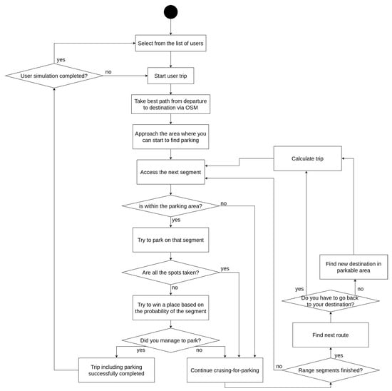
Figure 1.
Trip simulation flow diagram.
The decisions taken in step 6 (“Is within the parking area?”), 12 (“Range segments finished?”) and 14 (“Do you have to go back to your destination?”) are based on a probability value that depends on the user model involved. For example, a buyer user, as he or she wishes to park as close as possible to the destination, regardless of the time spent on cruising, will decide on “yes” at step 14 more often than a worker user.
As anticipated, the decision made in step 8 (“Are all the spots taken?”) refers to the parking availability of the involved segment, which depends on the previous simulations. The analysis of traffic and the possibility of two or more drivers influencing each other simulations in ways other than parking availability is not part of this study, as not considered essential for the success of the proposed task.
At step 15 (“Find new destination in the parkable area”), the simulator decides where to head the driver if no spot is available in the current segment. The driver is directed towards a new point in front of them, chosen randomly. A function, given the terrestrial axes, firstly calculates the car’s direction (bearing) and then moves it to the new destination point (Figure 2).
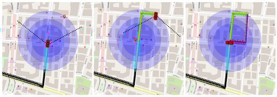
Figure 2.
Example of a moving driver.
4. Data Collection
We exploited the Cruising for Parking Simulator (CPS) described in the previous section to populate the parking spots in the area through a large amount of cruising for parking trips.
The proposed experiment was done in Rome, Italy, in the city area of San Giovanni. In the experiment, we deduced the ground truth about parking lot availability by combining the information offered by the EasyPark application [26] with the data collected through interviews and on-place observations.
We simulated 40 users moving for 200 weeks in the city area of San Giovanni in Rome. The drivers’ types and schedules were derived by interviewing an equal number of people who frequent the San Giovanni area. We considered 60 road segments in the area; Figure 3a,b show the ground truth about parking availability levels of the area during the first and second period of the simulation.
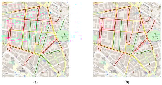
Figure 3.
San Giovanni (Rome, Italy) area’s segments. (a) Parking availability at 07:00–10:00. (b) Parking availability at 10:00–13:00.
Table 5 shows the number of segments and the colour (Green, Yellow or Red) matched for each time slot, while Table 6 presents the different types of users involved and their schedules. Depending on the driver’s type, these schedules were eventually repeated on different weekdays.
Table 5.
Color per time period.
Table 6.
Type of users for time periods.
During this simulation session, 27,603 trips were collected. For each trip, information about parking and unparking actions were gathered (Table 7 shows how parking and unparking actions are distributed by time slots). Each trip also contained information of each segment the driver passed without finding a parking spot (cruising actions), increasing the information available (136,687 total actions).
Table 7.
Park and Unpark actions.
Map-Matching
Before building the training dataset, we applied a Map-Matching step to the collected data.
Each trip T is composed of a sequence of ordered triplets (xk, yk, tk) each of which represents the location (xk = latitude, yk = longitude) of the user at that time tk. The Map-Matching goal is to transform the travel points into respective road segments. Such a process entails a number of benefits.
Firstly, it allows not to lose the accuracy given by the coordinates of the points. At the same time, it allows reducing the requirement for storage space and the computational time significantly [27].
Moreover, matching map coordinates to segments helps to solve problems given by inaccurate GPS locations by repositioning them correctly on the road [28].
Finally, in the case studied, Map-Matching is helpful to recognize circling more rapidly (cruising over the same segment multiple times).
Each point trip point is associated with a certain edge, corresponding to a part of the road. The Map-Matching process involves the transformation of GPS data into a network of road segments, so as to be able to recompose the exact path that the user has traveled on the map to reach the destination. Then the final transformation allows to pass from a trip T<(x1, y1, t1), (x2, y2, t2), …, (xn, yn, tn)> to a set of edges T<e1, e2, …, ek> where ej represents the edge hit in the path. Clearly, since there are many points corresponding to the same segment, the amount of data is drastically reduced.
As seen from the example (Figure 4), Map-Matching transformed the points of a trip into respective segments. We significantly reduced the collected points from 274 units to only nine segments, avoiding losing helpful information.
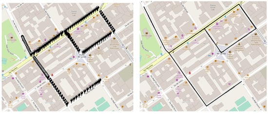
Figure 4.
Map-Matching example.
5. Dataset Building and Features Extraction
Once a significant amount of trips were collected, it was necessary to understand how to exploit them to extract the data that would help train the classifier. The literature about parking availability classification mainly focuses on the amount of parking and unparking, giving little importance (also due to lack of information) to the complete trip that interested the given segment. Instead, we aimed to exploit the information before parking to identify a road segment’s current situation.
While building the dataset, we aimed to collect generalized data about segments’ history. In this phase, we considered all 15 time periods (07:00–22:00) multiplied by the five weekdays, leading to the study of 75 different periods. For each period, we assembled the history of each segment by looking at the trips that involved the segment.
After the map-matching step, a trip is represented as a collection of segments, and each segment is part of the trip due to three possible actions: parking, unparking and cruising. A fourth action that can overlap with the others is circling, which represents a driver crossing the same segment multiple times.
We finally extracted the following ten features for each segment at a given time slot by observing the variance of these actions over the complete simulation, per trip and day. Over the 4500 possible combinations, the resulting dataset counts 761 samples, ignoring segments with zero actions.
5.1. Global Features
- Total Parking MeanFor all days assessed, total amount of parking spaces found on that segment with respect to the total number of times drivers have tried to park.
- Total Cruising MeanFor all days assessed, total amount of times no parking space was found on that segment with respect to the total number of times drivers have tried to park.
- Total Unparking MeanRatio of the total number of unparks over the number of days assessed.
5.1.1. In-Trip Features
- In-Trip Parking MeanRatio between the sum of the ratios between trips in which a park was found on that segment and trips in which a park was searched on that segment, and number of trips that involved that segment.
- In-Trip Cruising MeanRatio between the sum of the ratios between trips in which a park was not found on that segment and trips in which a park was searched on that segment, and number of trips that involved that segment.
- In-Trip Circling MeanRatio between the sum of trips in which the driver passed multiple times over that segment and number of trips that involved that segment.
5.1.2. In-Day Features
This type of feature calculates the number of total parking and cruising actions on the same day to limit the chance of anomalies, e.g., holidays, works in progress on that road, or other particular cases.
- In-Day Parking MeanThe number of parking events on each day is calculated (t is the time slot). This makes it possible to balance the possibility that, on a given day, one has only parked on a segment for a certain condition and to limit this information if it is not valid for all days.
- In-Day Cruising MeanThe number of passages occurred on each day is calculated. This makes it possible to balance the possibility that on a given day you have only passed on a segment for a certain condition and to be able to limit this information if it is not valid for all days.
5.1.3. Distance Features
Finally, the last two features refer to the distance separating the segment under consideration, on which the driver has parked, and the final destination.
- Parking Distance MeanMean distance between the segment on which drivers have parked and the destination they were looking for.
- Time Distance MeanMean walk time distance between the segment on which drivers have parked and the destination they were looking for.
6. Machine Learning Models
This study aims to generate a model to classify the Parking Availability Level of a given segment in a specified time slot. The possible outputs will therefore be three: Green, Yellow, or Red.
We trained and tested four supervised machine learning models (K-Nearest Neighbors, Gradient Boosting, Random Forest, Artificial Neural Network). All models receive the history of a segment and return a numerical value (0—green, 1—yellow, 2—red) to classify the Parking Availability Level of that segment on the specified time slot.
We made the following two observations during the training phase. First, by looking at the graph in Figure 5, it is possible to appreciate the validity of the parkedmean feature picked to train the model. In the case of the green label, the number of successful parking actions is high, while the opposite is true for the red label. Yellow, as expected, is positioned in the middle. The same can be noted for cruising and circling features.
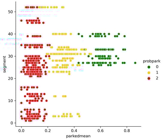
Figure 5.
Probability of the feature parkedmean to happen, in each segment, related to the three levels of availability.
Secondly, by analyzing the data, we noted that a few actions over a segment might affect the reliability of the features extracted from it. In fact, evaluating the risk and the possibility that a kind of “luck” influences the parking search is necessary in these cases. The user can find a parking space on a street that is always full; on the contrary, in the worst-case scenario, they cannot find it on a street that is usually highly available. For this reason, we carried out five trials with different minimum values for the number of actions required to consider a segment. From Table 8, it is possible to observe how the training accuracy grows as the number of actions evaluated increases. Hence, we decided to pick 30 as the minimum number of actions per segment, as it seems the best balance between a low threshold and a reasonable accuracy.
Table 8.
Test on the number of actions selected.
Models Performance
We split the complete dataset for training (70%) and test (30%).
During test evaluation, all models performed well, achieving over 90% of accuracy and therefore letting us validate the applicability of the data produced by the CPS. However, the four models also obtained very similar results, as shown by metrics in Table 9, Table 10, Table 11 and Table 12, and in confusion matrices Figure 6, Figure 7, Figure 8 and Figure 9.
Table 9.
ANN metrics on test-set.
Table 10.
KNN metrics on test-set.
Table 11.
Random forest metrics on test-set.
Table 12.
Gradient boosting tree metrics on test-set.
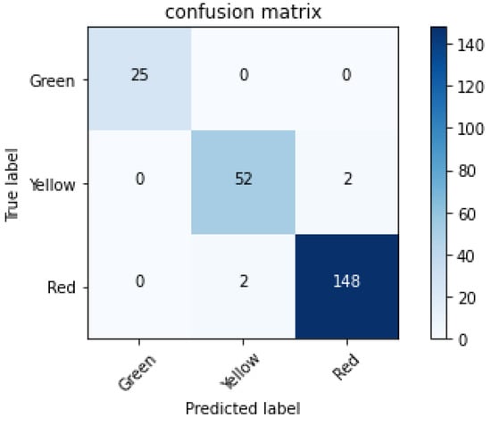
Figure 6.
ANN confusion matrix on test-set.
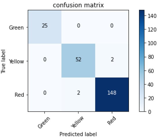
Figure 7.
KNN confusion matrix on test-set.
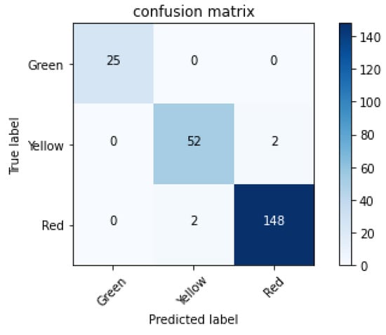
Figure 8.
Random Forest confusion matrix on test-set.
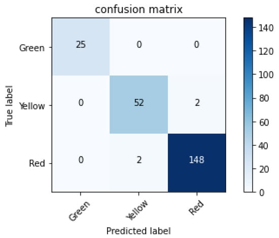
Figure 9.
Gradient boosting tree confusion matrix on test-set.
7. Experiment
To further evaluate the four models in the problem of classify the parking availability of a street segment, we designed an additional test case. The results presented in the previous section refer to the performance of the all the models trained and tested on data generated by the simulator in a session over the area of San Giovanni. During the following test case, the aim was to test the models on different data.
We generated new trips using the simulator in a different city area called San Lorenzo. As in the previous zone, the simulator inputs were decided based on on-site behavioral observations combined with data retrieved from EasyPark [26]. The simulation counted 40 users for 150 weeks. At the end of the simulation, we processed these trips to extract a new testing dataset.
San Lorenzo differs from San Giovanni as it is a smaller and more traffic-congested neighborhood (Figure 10). Sixty-one segments were identified and studied over five time periods for seven days. Out of the 2135 possible combinations of segments, 653 were selected as those involved in at least 30 actions. The ground truth data coincided with the simulator inputs.
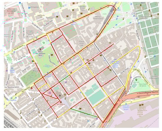
Figure 10.
San Lorenzo ground truth Parking Availability.
8. Results Discussion
The results achieved by the models in this test case were very high, reaching 97% of accuracy. From the confusion matrices (Figure 11, Figure 12, Figure 13 and Figure 14), it is also possible to note that errors, if any, always occur between yellow and another color, which is a less severe problem. It never happens that a green label is confused with a red one or vice versa.
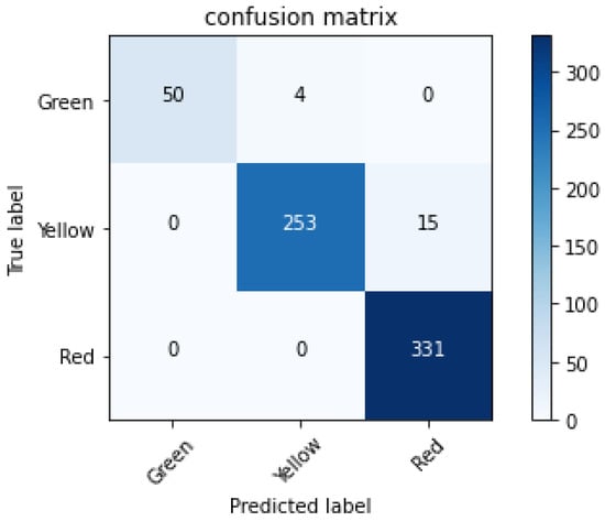
Figure 11.
ANN confusion matrix on San Lorenzo test case.

Figure 12.
KNN confusion matrix on San Lorenzo test case.
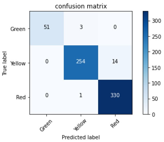
Figure 13.
Random Forest confusion matrix on San Lorenzo test case.
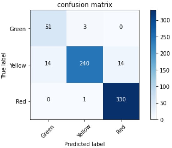
Figure 14.
Gradient boosting tree confusion matrix on San Lorenzo test case.
As happened during the first training and testing phase, the four considered models obtained very high and very similar results. The metrics adopted to evaluate the models are accuracy, precision, recall, and f1-score. The results are shown in Table 13, Table 14, Table 15 and Table 16.
Table 13.
ANN metrics on San Lorenzo test case.
Table 14.
KNN metrics on San Lorenzo test case.
Table 15.
Random forest metrics on San Lorenzo test case.
Table 16.
Gradient boosting tree metrics on San Lorenzo test case.
Regarding accuracy, the best models are Random Forest and ANN, with 97%, followed by KNN (96%) and GB (95%).
Regarding precision in the classification of labels 0, 1 and 2, Random Forest and KNN reach the highest values (1.00, 0.98, 0.96 and 1.00, 0.99 and 0.94, respectively), followed by ANN (0.96, 0.98, 0.96) and GB, with the worst performance in recognizing the 0 label (0.78, 0.98, 0.96).
The recall values again see Random Forest and KNN as the best models (all values between 0.92 and 1.00), followed by ANN and GB with a few hundredths of a waste. Finally, even for the f1-score values the best models were RF and KNN (0.97–0.98 and 0.95–0.98, respectively), followed by ANN (0.92–0.98) and finally GB (0.86–0.98).
In conclusion, despite the difference between the performances obtained being centesimal, the GB is the worst model in all comparisons. The RF, on the other hand, always stands out as the best result. The ANN, a structurally more sophisticated model, is equal to the RF for accuracy but performs slightly worse according to the other metrics.
Overall, the chosen models performed well in the problem of classifying the level of parking availability of a street segment and confirm the possibility of designing a Parking Availability Classifier that relies on data collectible by smartphone sensors. Compared to other studies that adopted the same evaluation metric (accuracy) but used different sources of data and environments, our models performed better (97% against the 94.37% of [15], the 81% of [16], and the 87.82% of [17]).
9. Applicability
In the previous sections, we presented a Parking Availability Classifier trained on data comparable to that collected through smartphone sensors. Our work applies to smart-parking apps that aim to ease the users’ cruising-for-parking phase by providing them with real-time information on parking availability.
Making such an evaluation is challenging, as it requires collecting data about information that can change over time and requires on-site validation. As mentioned in Section 2, literature offers a great variety of approaches, but rarely do they rely on smartphones’ sensors only. Concerning the work carried by [20], we improved the precision from area to street segment level, relying on a less populated dataset than the Google one.
In future works, we aim to implement the prediction of the segments’ parking availability level on the prototype smart-parking app. By relying on smartphones’ sensors only, users will collect data about parking, unparking, and cruising actions, which will be processed into segments’ history information and given to the PAC to predict parking availability.
10. Conclusions
The proposed work aimed to correctly classify the parking availability on a given road on a segment level.
First, using the CPS we developed, we generated a large amount of realistic data about cruising, parking, and unparking events in the San Giovanni city area of Rome.
Once sufficient data was generated, some preprocessing steps were applied to build a training dataset for the machine learning models. This phase included applying map-matching techniques to the collected trip data, identifying ten features, and a dataset containing 761 segment samples.
We trained four machine learning models to classify the availability of on-street parking for a given road segment. All models performed well both in the training and testing phases.
To further evaluate the four models, we generated simulated data about 61 segments of a different city area (San Lorenzo, Rome) that differs from San Giovanni as it is a smaller and more traffic-congested neighbor. The results achieved by the models in this test case were very high, reaching 97% accuracy for all the street segments where we collected 30 or more user actions.
As the four models obtained very high results, especially the RF and the ANN, we confirmed that it is possible to design a PAC based on data collectible by smartphones.
11. Ongoing Work
Our current and future research work is twofold. First, we developed a prototype smartphone application and we are going to collect a significant amount of actual data to test our models. We plan to run tests in other zones to evaluate the model scalability to the entire city and the portability to other urban areas without repeating the user behavior analysis.
Secondly, we will consider other factors that may further refine the simulations, making them even more realistic. Examples are traffic flow that traverses the area without looking for parking, weather conditions, and events that may alter the prediction of a weekday on particular occasions.
Author Contributions
E.B.: Data curation, Resources, Software, Supervision, Writing—review & editing. A.B. (Andrea Berti): Conceptualization, Formal analysis, Investigation, Methodology, Software, Visualization, Validation, Writing—original draft. A.B. (Alba Bisante): Software, Supervision, Visualization, Writing—review & editing. A.M.: Conceptualization, Formal analysis, Investigation, Methodology, Software, Visualization, Validation, Writing—original draft. E.P.: Conceptualization, Funding acquisition, Project administration, Resources, Supervision, Writing—review & editing. All authors have read and agreed to the published version of the manuscript.
Funding
This research was funded by Ministero dell’Università e della Ricerca grant Dipartimenti dieccellenza 2018–2022 of the Department of Computer Science of Sapienza University of Rome and by Sapienza University of Rome grant Progetti di Ateneo 2019.
Data Availability Statement
Data and algorithms presented in this study are openly available in FigShare at: https://doi.org/10.6084/m9.figshare.20331708 (accessed on 19 September 2022).
Conflicts of Interest
The authors declare no conflict of interest.
Abbreviations
The following abbreviations are used in this manuscript:
| PAC | Parking Availability Classifier |
| CPS | Cruising for Parking Simulator |
| IoT | Internet-of-Things |
| ML | Machine Learning |
| NN | Neural Networks |
| RNN | Recurrent Neural Networks |
| DL | Deep Learning |
| LSTM | Long-Short Term Memory |
| dConvLSTM-DCM | dual Convolutional LSTM with Dense Convolutional Network |
| CNN | Convolutional Neural Networks |
| GRU | Gated Recurring Unit |
| DELM | Deep Extreme Learning Machine |
| RF | Random Forest |
| DT | Decision Tree |
| KNN | K-Nearest Neighbor |
| MLP | Multilayer Perceptron |
| SARIMAX | Seasonal Auto-Regressive Integrated Moving Average with |
| exogenous variables | |
| DNN | Deep Neural Network |
| GB | Gradient Boosting |
| EL | Ensamble Learning |
| ANN | Artificial Neural Network |
| PRR | Parking Remaining Ratio |
References
- Shoup, D.C. Cruising for parking. Transp. Policy 2006, 13, 479–486. [Google Scholar] [CrossRef]
- Bogoslavskyi, I.; Spinello, L.; Burgard, W.; Stachniss, C. Where to park? minimizing the expected time to find a parking space. In Proceedings of the 2015 IEEE International Conference on Robotics and Automation (ICRA), Seattle, WA, USA, 26–30 May 2015; pp. 2147–2152. [Google Scholar] [CrossRef]
- Marso, K.; Macko, D. A New Parking-Space Detection System Using Prototyping Devices and Bluetooth Low Energy Communication. Int. J. Eng. Technol. Innov. 2019, 9, 108–118. [Google Scholar]
- Tiedemann, T.; Vogele, K.; Metzen, K. Concept of a Data Thread Based Parking Space Occupancy Prediction in a Berlin Pilot Region. In Proceedings of the Workshops at the Twenty-Ninth AAAI Conference on Artificial Intelligence, Austin, TX, USA, 25–30 January 2015. [Google Scholar]
- Shao, S.; Salim, F.D.; Gu, T.; Dinh, N.-T.; Chan, J. Traveling Officer Problem: Managing Car Parking Violations Efficiently Using Sensor Data. IEEE Internet Things J. 2018, 5, 802–810. [Google Scholar] [CrossRef]
- Panizzi, E.; Bisante, A. Private or Public Parking Type Classifier on the Driver’s Smartphone. Procedia Comput. Sci. 2022, 198, 231–236. [Google Scholar] [CrossRef]
- Wu, M.C.; Yeh, M.C. Early Detection of Vacant Parking Spaces Using Dashcam Videos. In Proceedings of the AAAI Conference on Artificial Intelligence, Honolulu, HI, USA, 27 January–1 February 2019; Volume 33, pp. 9613–9618. [Google Scholar] [CrossRef]
- Zheng, Y.; Rajasegarar, S.; Leckie, C. Parking availability prediction for sensor-enabled car parks in smart cities. In Proceedings of the 2015 IEEE 10th International Conference on Intelligent Sensors, Sensor Networks and Information Processing, ISSNIP 2015, Singapore, 7–9 April 2015. [Google Scholar] [CrossRef]
- Vlahogianni, E.; Kepaptsoglou, K.; Tsetsos, V.; Karlaftis, M. A Real-Time Parking Prediction System for Smart Cities. J. Intell. Transp. Syst. 2015, 20, 192–204. [Google Scholar] [CrossRef]
- Bassetti, E.; Luciani, A.; Panizzi, E. ML Classification of Car Parking with Implicit Interaction on the Driver’s Smartphone. In Proceedings of the IFIP Conference on Human–Computer Interaction, Bari, Italy, 30 August–3 September 2021; Springer: Berlin/Heidelberg, Germany, 2021; pp. 291–299. [Google Scholar]
- Provoost, J.C.; Kamilaris, A.; Wismans, L.J.; van der Drift, S.J.; van Keulen, M. Predicting parking occupancy via machine learning in the web of things. Internet Things 2020, 12, 100301. [Google Scholar] [CrossRef]
- Feng, Y.; Xu, Y.; Hu, Q.; Krishnamoorthy, S.; Tang, Z. Predicting vacant parking space availability zone-wisely: A hybrid deep learning approach. Complex Intell. Syst. 2022, 1–17. [Google Scholar] [CrossRef]
- Yang, S.; Ma, W.; Pi, X.; Qian, S. A deep learning approach to real-time parking occupancy prediction in transportation networks incorporating multiple spatio-temporal data sources. Transp. Res. Part C Emerg. Technol. 2019, 107, 248–265. [Google Scholar] [CrossRef]
- Arjona, J.; Linares, M.; Casanovas-Garcia, J.; Vázquez, J.J. Improving Parking Availability Information Using Deep Learning Techniques. Transp. Res. Procedia 2020, 47, 385–392. [Google Scholar] [CrossRef]
- Siddiqui, S.; Khan, M.; Abbas, S.; Khan, M. Smart Occupancy Detection for Road Traffic Parking using Deep Extreme Learning Machine. J. King Saud Univ. Comput. Inf. Sci. 2020, 34, 727–733. [Google Scholar] [CrossRef]
- Inam, S.; Mahmood, A.; Khatoon, S.; Alshamari, M.; Nawaz, N. Multisource Data Integration and Comparative Analysis of Machine Learning Models for On-Street Parking Prediction. Sustainability 2022, 14, 7317. [Google Scholar] [CrossRef]
- Awan, F.M.; Saleem, Y.; Minerva, R.; Crespi, N. A comparative analysis of machine/deep learning models for parking space availability prediction. Sensors 2020, 20, 322. [Google Scholar] [CrossRef] [PubMed]
- Paidi, V. Short-term prediction of parking availability in an open parking lot. J. Intell. Syst. 2022, 31, 541–554. [Google Scholar] [CrossRef]
- Errousso, H.; Malhene, N.; Benhadou, S.; Medromi, H. Predicting car park availability for a better delivery bay management. Procedia Comput. Sci. 2020, 170, 203–210. [Google Scholar] [CrossRef]
- Arora, N.; Cook, J.; Kumar, R.; Kuznetsov, I.; Li, Y.; Liang, H.J.; Miller, A.; Tomkins, A.; Tsogsuren, I.; Wang, Y. Hard to Park? Estimating Parking Difficulty at Scale. In Proceedings of the KDD’19: 25th ACM SIGKDD International Conference on Knowledge Discovery & Data Mining, Anchorage, AK, USA, 4–8 August 2019; Association for Computing Machinery: New York, NY, USA, 2019; pp. 2296–2304. [Google Scholar] [CrossRef]
- eParkomat. eParkomat: We Predict Real-Time Parking Situation. Available online: https://www.eparkomat.com (accessed on 19 September 2022).
- Rong, Y.; Xu, Z.; Yan, R.; Ma, X. Du-Parking: Spatio-Temporal Big Data Tells You Realtime Parking Availability. In Proceedings of the 24th ACM SIGKDD International Conference on Knowledge Discovery & Data Mining, London, UK, 19–23 August 2018; pp. 646–654. [Google Scholar] [CrossRef]
- ParkMobile. How Does the Parking Availability Feature Work. Available online: https://support.parkmobile.io/hc/en-us/articles/360001341732-How-does-the-Parking-Availability-feature-work- (accessed on 19 September 2022).
- Bonsall, P.; Palmer, I. Modelling drivers’ car parking behaviour using data from a travel choice simulator. Transp. Res. Part C Emerg. Technol. 2004, 12, 321–347. [Google Scholar] [CrossRef]
- OpenStreetMap Contributors. Planet Dump. 2017. Available online: https://planet.osm.org;https://www.openstreetmap.org (accessed on 19 September 2022).
- EasyPark. Available online: https://easyparkgroup.com (accessed on 19 September 2022).
- Tiwari, V.; Sarda, N.L. A faster way to establish trip similarity. In Proceedings of the Conference on Geo-spatial Technologies & Applications, Valencia, Spain, 30 January–4 February 2012. [Google Scholar]
- Froehlich, J.; Krumm, J. Route Prediction from Trip Observations. In Proceedings of the Society of Automotive Engineers (SAE) 2008 World Congress, Detroit, MI, USA, 14–17 April 2008. [Google Scholar]


Publisher’s Note: MDPI stays neutral with regard to jurisdictional claims in published maps and institutional affiliations. |
© 2022 by the authors. Licensee MDPI, Basel, Switzerland. This article is an open access article distributed under the terms and conditions of the Creative Commons Attribution (CC BY) license (https://creativecommons.org/licenses/by/4.0/).