1. Introduction
Increased population in recent years around the globe resulted in the over-exploitation of fossil fuels, especially in the electricity generation and transportation sectors. An alarming effect on the environment is the depletion of the ozone layer with increased emission of greenhouse gases (GHG), which led world governments to take action in reducing the consumption of fossil fuels and replacing them with renewable energy sources (RES). However, the penetration of RES results in instability in the operation [
1] of its stochastic nature. Thereby, energy storage systems (ESS) are opted to compensate for the intermittent supply of renewable energy sources using power electronic converter controllers [
2]. The dynamic demand cannot be fully met by energy storage devices due to their expensive investment and degradation factors. Hence, fuel-based generators are also introduced to the network to support cost-effectiveness in operation and consistency. On the other hand, there has been a steady increase in the utilization of electric vehicles (EVs) for their ecological benefits. They also have the capability to act as reserves for the distributed generators due to their storage capacity when connected to the grid [
3]. Although, there is a rising complication in the distribution system stability due to the inconsistent nature of charging and discharging [
4], thus increasing the complexity of the microgrid to control with the integration of increasing components. The microgrid, which is an integral part of the smart grid, plays a key role in addressing the economic, environmental, efficiency, reliability, security, and stability-related aspects through the microgrid energy management system (MEMS).
An energy management system (EMS) is an automated software framework designed for the optimal performance of the microgrid. EMS maintains the balance between generation and demand considering the market price and meteorological data [
5]. Microgrid EMS is a hierarchical architecture consisting of three levels: tertiary, secondary, and primary, each with a different time scale of control [
6]. Many approaches have been proposed to solve the energy management in microgrids and a detailed review of the control approaches is presented in [
7]. To mention a few, an EMS is developed to analyze the power exchange with the grid by particle swarm optimization (PSO) to optimally schedule the generation and increase the profit margin [
8]. Genetic algorithm (GA)-based energy management is performed to increase the efficiency of the heating, ventilation, and air conditioning (HVAC) loads integrated with PV, wind generation, and storage [
9]. The thermal and power demands are scheduled in an islanded microgrid, formulated as a MILP problem to minimize the fuel cost and thermal comfort requirements [
10].
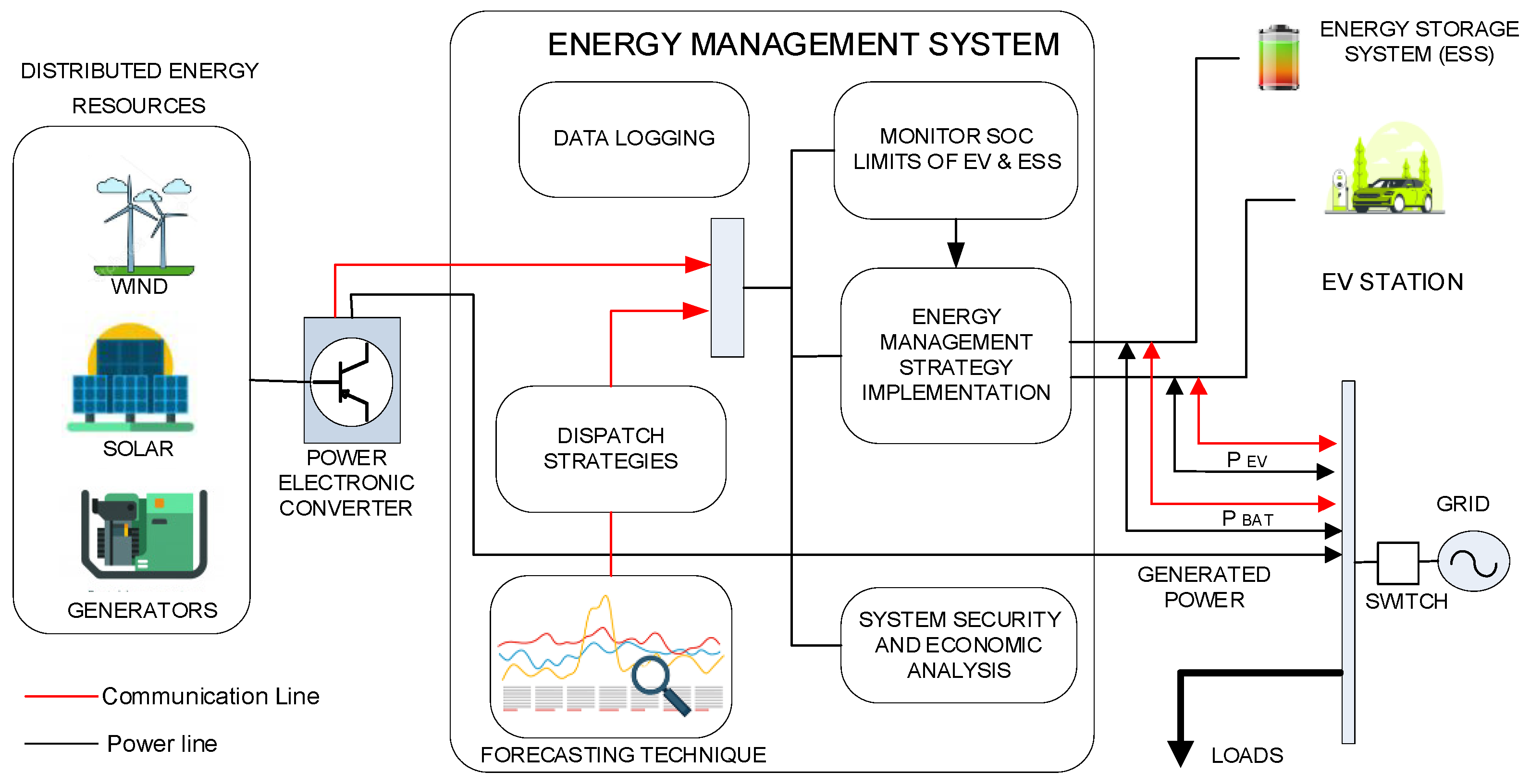
Figure 1 shows a typical energy management structure of a microgrid.
Forecasting is a crucial element in developing an energy management schedule. The prediction through historical data cannot provide accurate results as it consists of uncertainty due to forecasting errors [
11]. For uncertainty modeling in planning and operation, stochastic programming is commonly employed [
12]. In [
13], the authors have provided an updated evaluation of uncertainty modeling approaches in the energy management system. The day ahead energy management can increase its cost benefits through the inclusion of demand response.
Demand response (DR) is an extended part of EMS where the end-user response of load utilization is used by the utility company to schedule the load based on dynamic electricity pricing [
14]. The demand response programs are divided into two categories: incentive-based rates and time-based rates [
15]. Direct load control (DLC), auxiliary services market (A/S), interruptible/curtailable services (I/C), capacity market program (CAP), emergency demand response program (EDRP), and demand bidding (DB) are incentive-based programs [
16]. Customers in incentive-based schemes, such as I/C and CAP, are penalized if they do not curtail as directed. Consumers are encouraged to reduce loads at a curtailable price under the DB program, while the auxiliary services program allows customers to participate in the energy market via load curtailment. DLC and EDRP are voluntary programs; participants are not punished if they do not reduce their usage [
17]. The cost of time-based DR programs varies according to the cost of supplies for different time periods. Time-based and incentive-based systems can be combined to increase system efficiency [
18]. Algorithms have been developed [
19] for the DR program with consideration of limitations in their characteristics of modeling. A day-ahead shifting of load to acquire the least cost price of power while implying scheduled sources as exchange [
20], where DLC is used with no end-user control.
The user agrees willingly to support demand fluctuation in accordance with the utility demand response program. In [
21], a detailed review of demand response programs is mentioned A demand response pricing is developed to model the load shifting based on demand response according to the users for urban microgrids with the user-defined program [
22]. The limitation of this strategy is not having fixed demand response pricing but rather multi-user-based pricing which in practical scenarios can be affected by the increased communication traffic and storage every day. These approaches have performed demand response to control the home appliances through smart meter communication from the control center.
This paper proposes a novel strategy for the optimal load shifting of demand for day-ahead energy management with incentive/penalty pricing as support that allows the users to decide with a cautionary update on the equipment to be operated. This proposed methodology has the following key contributions; developing Hong’s two-point estimate scheme for the uncertainty parameter estimation, hybrid energy sources based multi-objective optimization approach to maintaining the state of charge in battery energy storage system (BESS) and EV charging station (EVCS), and developing a power management incentive pricing method for the optimization of shiftable demand response using genetic algorithm.
The paper structure is as follows:
Section 2 contains the problem formulation of the microgrid energy management problem which discusses cost function, mathematical modeling of the components, uncertain parameter, and optimization handling technique.
Section 3 consists of the proposed methodology approach. In
Section 4, the results and analysis of the proposed methodology are validated with comparison. Lastly,
Section 5 summarizes the findings of the study.
2. Methodology
Microgrid energy management is an algorithm to control the dynamic demand–supply balance under specified constraints. Generally, an EMS is formulated with one or many objectives to be achieved and is solved considering it as a nonlinear NP problem. The microgrid components need to be formulated into mathematical models for analysis. This section introduces the mathematical formulation of microgrids, uncertainty modeling, and methodologies opted.
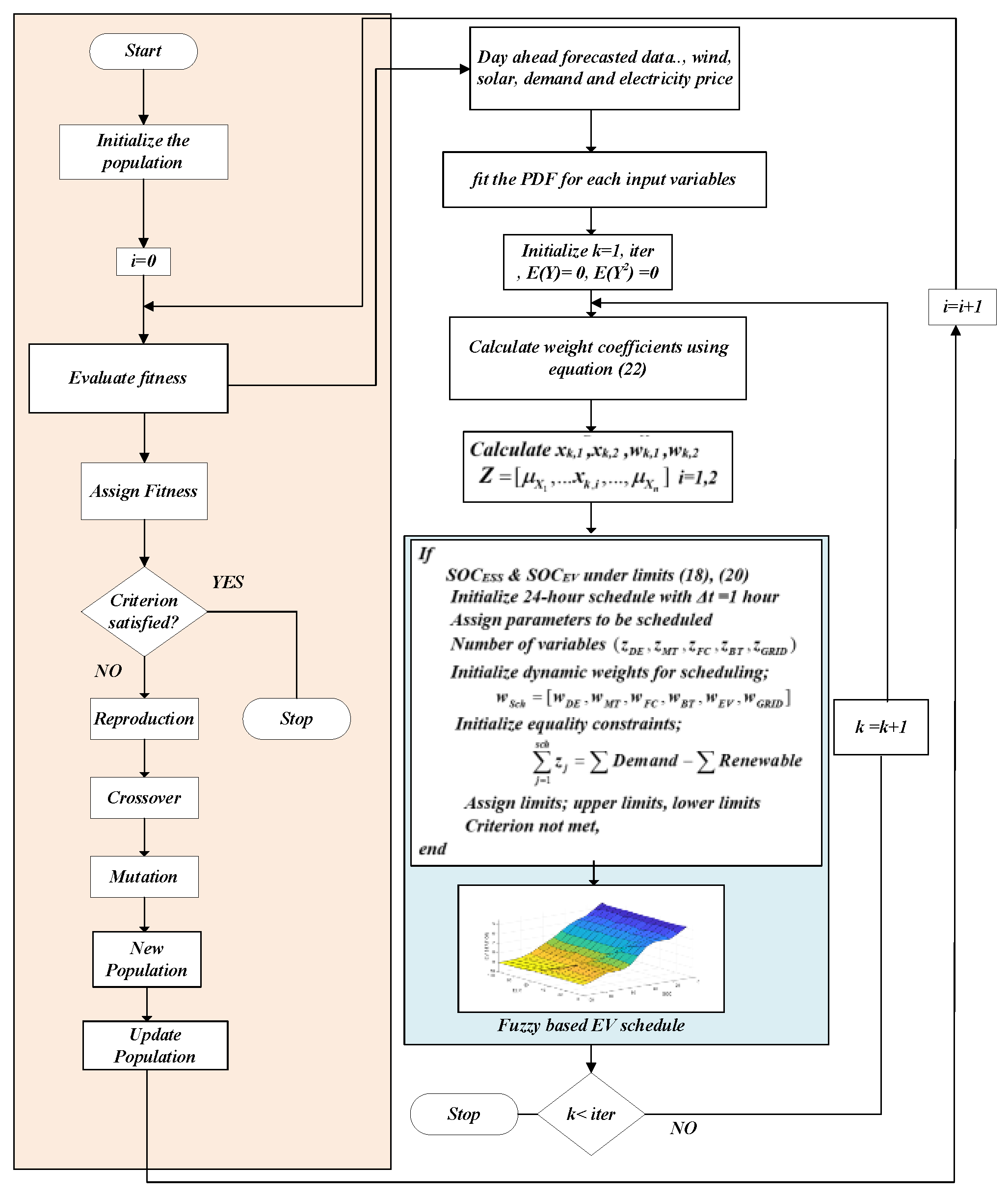
Figure 2 shows the methodology flow diagram.
2.1. Problem Formulation
This section discusses on mathematical modeling of the microgrid elements for energy management. Microgrid renewable consists of wind and solar generation. Renewable energy sources are intermittent sources that will depend on several parameters, among others: sunshine, temperature, wind speed, wind direction, season, etc. The microgrid analysis with intermittency, power converters, energy storage devices, dispatchable generators, and fluctuating load demand for energy management needs mathematical modeling of these components. This section provides an initial step toward an energy management framework with modeling elements of the microgrid. The study for a typical day is generated through the random behavior of the different renewable resources. For the case study, the hourly solar generation, wind generation, demand, and electricity price forecasting uncertainties are modeled by the probability density functions (PDF). From the forecasted data, the mean and standard deviation for each time segment is calculated, and from them, probability density functions are generated for each hour.
Wind generation is dependent on the velocity of the wind (
v) and the power curve of the wind turbine [
23]. For solar, the power generation depends on irradiance (
R) and ambient air temperature (
T) of the location the photovoltaic (PV) panels are installed [
10]. The power generated for solar (
PPV) and wind (
Pwd) at time period “
t” is calculated using Equation (1) to Equation (4). The variables of velocity (
vi,
vo,
vr) represent, cut-in, cut-off, and rated wind speeds(m/s). In solar,
k represents the manufacturer’s temperature power coefficient W/°C.
Rr represents the irradiance of the PV (1000 W/m
2). The efficiency of the power electronic converter and solar panel is represented as
ηPEC and
ηPV, respectively.
Battery storage or energy storage systems (BESS) in the microgrid support renewable sources’ intermittent power supply. Energy storage systems allow for obtaining benefits both in the technical area, including capacity markets [
19], as well as help to effectively use surplus energy with the use of coin-mining [
14]. The ESS charges or discharges according to the economic and energy requirements in the grid. The battery characteristics are based upon their
SOCt (state of charge at
t) which can be derived from the (5) and power consumed by the energy storage devices
PESS,t as (6).
Fuel-based generators comprise microturbine (MT), fuel cell (FC), and diesel generators (DE). These dispatchable sources are used to meet the demand in case of deficiency. These generators (
Pi) use the fuel as the driving force and the cost consumption is calculated as in Equation (7), where
ɑi,
bi, and
ci are the fuel cost coefficients.
The EVs are approximated to batteries during their operations at a charging station, the state of charge and energy consumption is calculated in an as single point as described in the Equations (8) and (9). The available storage capacity of an EV charging station is determined by various uncertain elements, such as the behavior of EV users, the arrival and departure timings of the cars, the distance traveled prior to their arrival, and the state of charge. An assumption is considered that the charging station participates as storage during the peak hours of traffic, i.e., during 07.00–21.00 h. A detailed driving pattern of PEV drivers is taken and represented as a normal PDF, which includes arrival, time of departure, and travel distance [
24].
The end users provide some flexibility in DR programs over to the aggregators for minimizing the billing cost or during the grid offline. Appliances can be categorized as shiftable or non-shiftable, which are controlled by independent smart meters for the period of usage. A maximum of about 30% of the total appliances in a microgrid can participate in a demand response program [
25].
In this article, a distribution system direct load control-based demand response program, which is an incentive-based model with dynamic pricing is considered. The user can use the controllable device with penalized price or use it for an incentive period. Implementation of the proposed DR program would curtail consumption in peak hours and increase prices. The dynamic price is modified according to the load shiftable (11).
Table 1 shows the devices that engage in demand response as well as their utilization times [
26].
2.2. Fitness Function
The energy management in this paper is a multi-objective NP minimizing problem with three aspects to handle as shown in (12), the first term is the overall cost which includes distribution generation startup and maintenance cost, the second term is the total power loss, and the third term is the greenhouse gases emissions from the generation units [
27]. Each objective is assigned weights
and their totality is unity, the weights prioritized
for the optimal performance of the system.
The objective function is analyzed with constraints of the power balance between the generator, storage, and demand as shown in (13), the power flow for the optimal power is performed using modified Newton Raphson as it gives faster convergence [
28]. The constraint for active power flow is shown in (14), the demand shift is shown in (15), the power exchange of energy storage systems in (16), and the power and state of charge of electric vehicles in (17) and (18), and voltage limit in (19).
2.3. Hong’s Two Point 2 m Estimate Method
Point estimate methods (PEM) are developed to compute the statistical moments of random variables by evaluating the distribution function of an uncertainty variable. The PEM uses the statistical data of input random variables to find the concentrations or central moments on
K points of the variable. The uncertainty in forecasted values differs from the real value as an error and function
F transmits the input random variables to the output variable. Such that the function f can be represented as,
F(20), where v is a set of variables and
pl (
l = 1, …,
m) of input uncertainty variable with probability distribution P
D. The
X and
Y represent the input and output values of the function.
The
Kth concentration (
pl,k, wl,k), composes of location
pl,k, and weight
wl,k. In Hongs PEM, each random variable of
pl in the function
F is solved for
K times. The difference in the solution of each
pl is the location
pl,k, and the remaining input variables are assigned with their corresponding means. The total number of solutions for the function
F is
K ×
m [
29]. Hong’s 2 m method indicates the status of the location of the output parameters by producing two probability concentrations for each variable namely the weight factor and the location of the input random variable. For instance, consider
pl as the input parameter with certain probability distribution [
30].
To implement Hong’s 2 m method, initially specify the number of inputs
m. Then, define the value
E(Yj) = 0 for the two moments, i.e.,
k = 2. Select the uncertain parameter
pl where
l states the uncertain variables in the system. Calculate the skewness of the system as in (21),
where
,
M is the observations and P is the probability of the uncertain parameter
pl [
31]. With the skewness available, calculate the two standards and the estimated locations using (22) and (23), respectively.
Once the locations are obtained the deterministic function
for the
kth value is estimated and then the weights are calculated (24) and (25).
The updated values of the first and second moment are calculated for the output
Y as shown in (26). This gives us the value for an uncertain variable, repeat a similar procedure for the remaining variables. Finally, the predicted values and standard deviation of the output parameter are calculated using Equations (27) and (28) as the outcomes.
Hong’s 2 m method is adopted in this work for its simplicity, low computational burden, and real-value solutions for the concentration.
2.4. Fuzzy Approach for EVs Fleets Scheduling
Estimating the quantity of the charge/discharge power of the electric vehicles reduces the computational burden of the problem. The microgrid CC estimates the pattern of consumption and supply from the forecasted data of cost, load utilized, renewable generation, state of charge in batteries, and electric vehicle charging station as part of the decision-making process [
32].
A fuzzy inference system is designed for making decisions on charging/discharging according to the state of charge (SOCEVCS) of EVs, estimated total price (ETP), and estimated load remaining (ELR) during the period. The fuzzy membership functions are modeled in degrees of the input pattern and output pattern. The fuzzy inference consists of 36 rules written for the process, ELR and EEP have 3 functions high, medium, low (H, M, L), and SOCEV has 4 functions very low, low, average, high (VL, L) and output observes 3 functions charge, neutral, discharge (C, N, D). The priorities of the fuzzy rule set for charging when SOC is low, ELR and discharging to high SOC, ELR with ETP being allocated to medium or low on prior and high to latter set. The output fuzzy set is calculated by the fuzzy inference engine, and the charging and discharging rate is obtained through the defuzzification process to prepare the output signal using the center of mass method
2.5. Multi Objective Genetic Algorithm
Genetic algorithm is an evolution-based natural selection optimization, it has three main operations namely, crossover, mutation, and selection. In every iteration of the problem, it uses generated population as solutions which are created randomly at the initial step. A chromosome or string is the encoded version of each solution with either a single or a sequence of values. Each chromosome in the population is assigned a fitness value using fitness evaluation, which is used for selecting the fittest chromosomes in the population for the mating pool. The crossover of the two chromosomes produces an offspring or a new solution through swapping. Crossover improves the convergence while exploiting the search space with a high probability rate (0.8–0.95). The new chromosomes kept in the offspring pool are randomly changed by flipping genes. The further randomness operation is a mutation that has a low probability (0.001–0.05). The high crossover and low mutation probability provide a high degree of mixing and exploitation and lower exploration, in other terms, it has faster convergence and reaches global optimum [
33].
The generated new solution is subjected to fitness evaluation of the desired objectives of the problem. The selection of the fittest chromosome provides the best solution to the population and is further passed on to the next generation known as elitism. The elite pool gives the best solution and the other chromosomes that are present are replaced by chromosomes of the offspring pool. Randomly generated chromosomes are introduced if the offspring pool has a deficiency of chromosomes. The continuous process of generations provides the best fittest candidate for the solution at the termination of the optimization. In [
34], the author has provided different methods and operations involving crossover, mutation, and selection (either by elitism or replacement).
In this paper, GA is induced for the demand shifting for the day period, i.e., for 24 h with population size [
10,
24] and Rowlette wheel selection with a maximum deviation in a change of 0.3 to minimize the total cost fitness of the problem. Out of many algorithms, the GA is chosen for faster convergence and a robust approach. At every iteration, the algorithm generates a new population of demand shifted with the minimized objective function.
4. Results
This section provides the results of two case studies based on the above-mentioned strategy. The simulation study of energy management is grid-connected with two scenarios on utilization of demand response while the latter case study is in islanded mode with similar scenario studies. This section presents simulation outcomes with GA and MILP for the hybrid energy management of the microgrid considering uncertainties. These uncertainties are handled by Hong’s 2 m point estimate method. For analysis of the above methodologies, CIRGE European benchmark 14-bus low voltage microgrid test distribution system is taken [
35]. Aggregated load demand consists of residential users with a consumption of 150 kW, a medium industrial workshop with 100 kW, and a commercial user of 50 kW as per the test system. For generalization of the urban microgrid, an EV charging station is assumed to be located in a commercial area with 25 charging ports in mode 2 of operation, i.e., a 6.6 kW battery is fully charged in 4 h considering no charge.
4.1. Test System
The microgrid distribution system includes a 50 kW diesel generator, 10 kW fuel cell, 20 kW microturbine, two 50 kW wind turbines, a 0.1 MW PV array, and four 25 kWh batteries connected in parallel. The overall energy storage devices have a charging and discharging capacity of 100 kW, while the electric car station has a charging and discharging power of 10 kW. The total load is 2 MW at peak and the total energy demand for an average weekday day is 3488 kWh. The power factor of all loads is assumed to be 0.85 [
36].
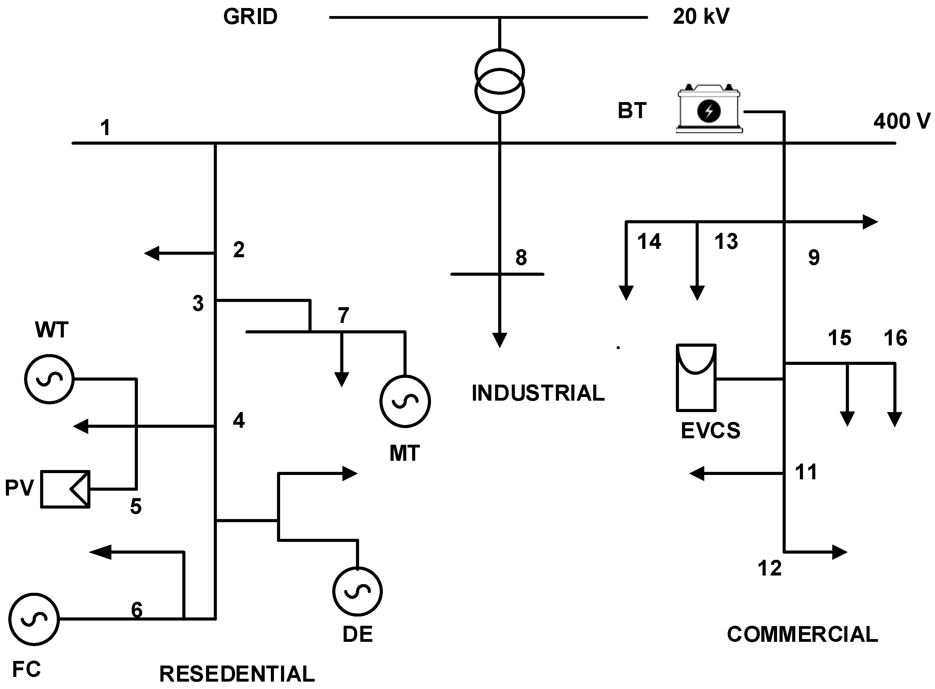
Figure 4 shows 14 bus CIRGE low-voltage microgrid.
The cost functions of the distributed generators along with the electric vehicle charging station are also included. It is assumed that the energy storages and electric vehicles are vulnerable and discharged only during the islanded or emergency mode [
37]. The forecasted data consists of solar irradiance, and wind velocity taken for the average forecasted month of 10 March 2022 in the West Godavari region, and hourly electricity price is taken from the online pricing platform [
38].
Table 3 provides the minimum and maximum generation, startup/running, bid coefficients, and the emissions quantity of the DG’s in the microgrid [
36]. In
Figure 5, the forecasted solar generation, wind generation, demand consumption, and demand bidding of electricity pricing for 24 h are shown.
4.2. Analysis
In grid-connected mode, the DGs work under the constraints of fulfilling the hourly demand. In this methodology, the utility is connected. Two scenarios are examined in light of the demand routing application. As the objective function for the assessment, the emission rate, cost, and power loss are evaluated accordingly. The state of charge of the energy storage systems and electric vehicles are taken as the reference limit constraints for the system to perform optimally in the islanded mode, considering the degradation and vulnerability of batteries this condition is assumed. The proposed methodology case study is performed in MATLAB with CPLEX integration using an i5 processor with 8 GB of RAM.
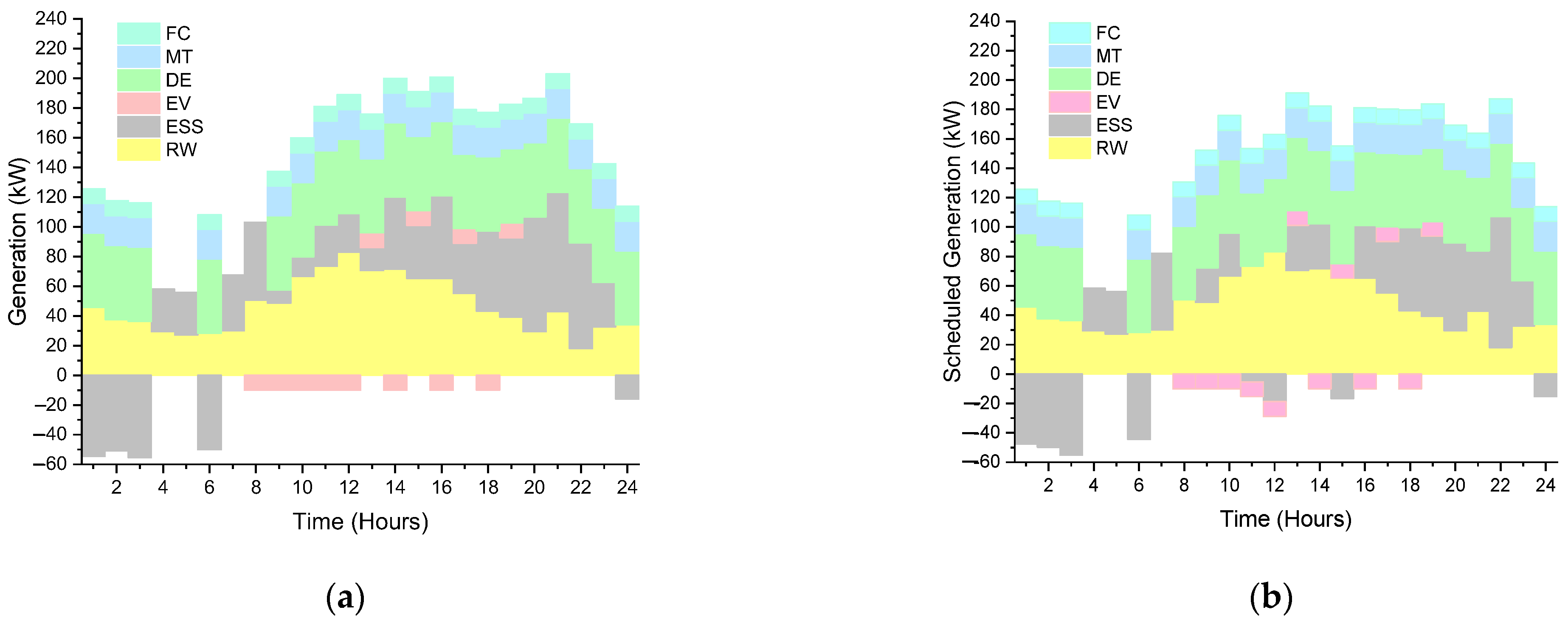
Scenario I: In this case, the microgrid undergoes energy management for 24 h period with demand scheduling and generation scheduling is performed optimally using the MILP. In this scenario, the scheduling is performed to reduce the dependency of the utility and compensate it with the dispatchable generators operating at optimum in consideration of the cost reduction. The total fitness cost of the problem is USD 1720.15 with an overall cost of the microgrid operation is USD 343.33 mean and standard deviation of 4.67%. The emission and power losses are 1533 kg and 140.61 kW as mean values with a standard deviation of 2.45% and 3.45%, respectively. The generation scheduling for a 24 h period is shown in
Figure 6a.
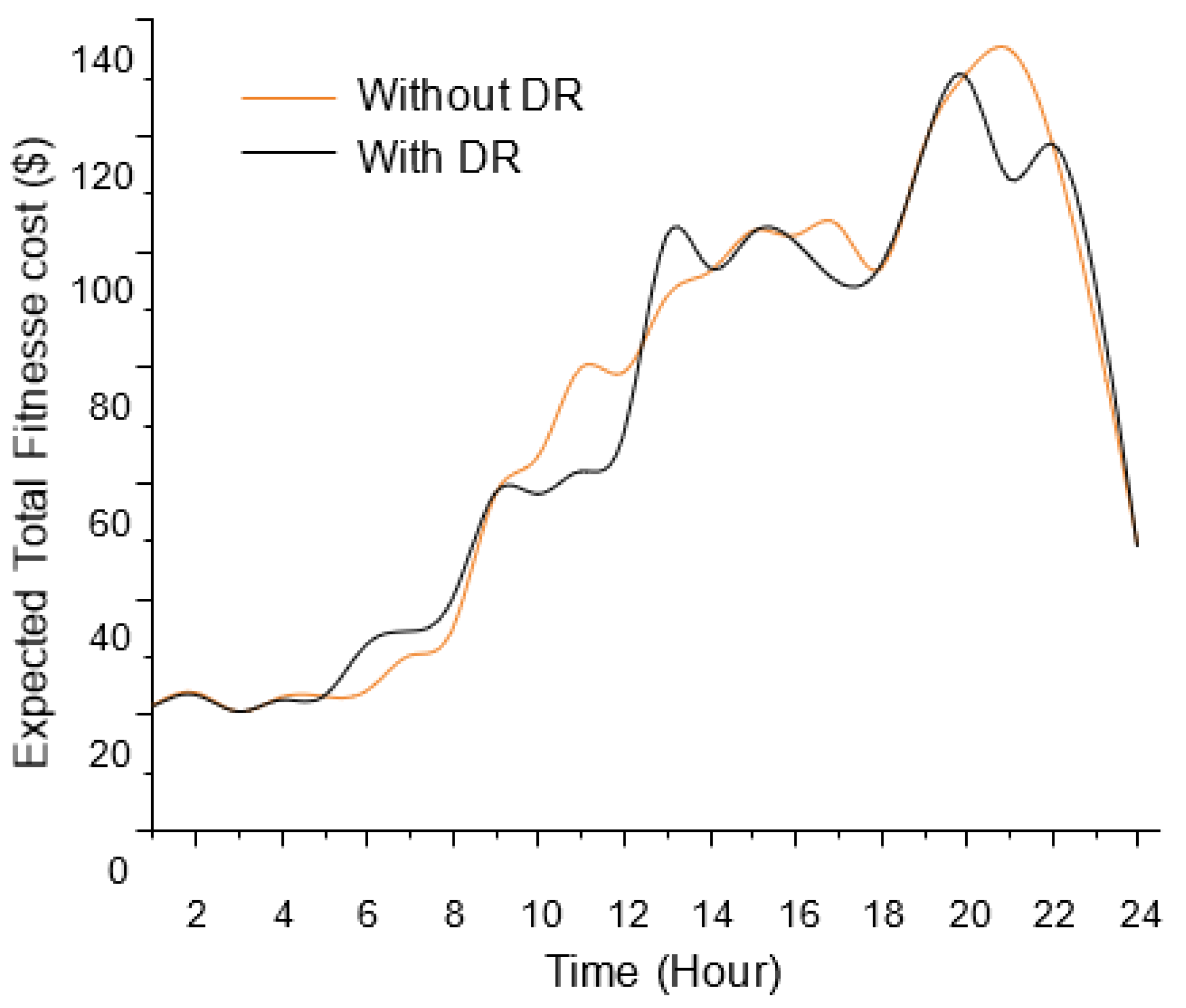
Scenario II: GA-based direct load control of DR application is performed in this case. With demand shifting the distributed generators are optimally scheduled which is shown in
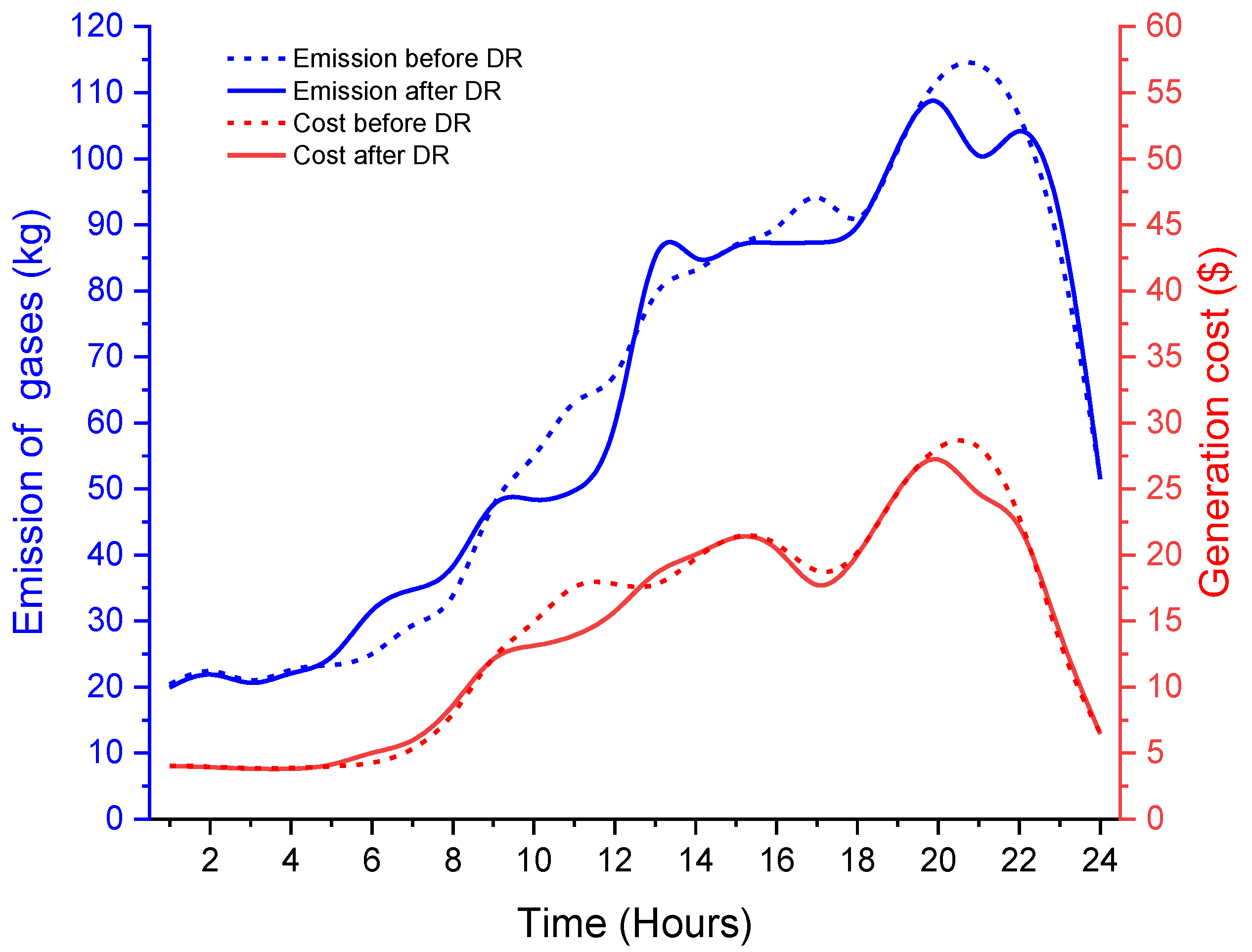
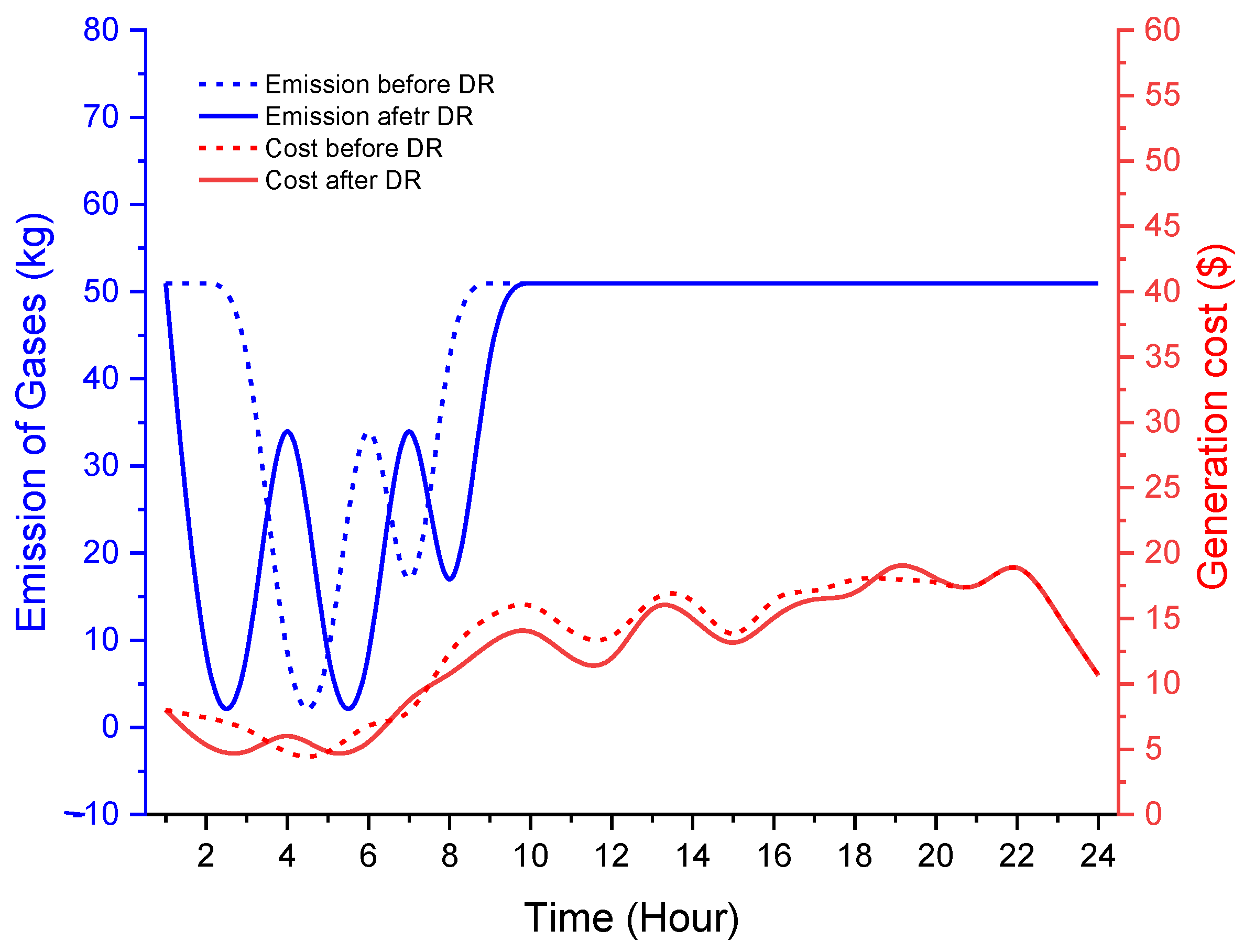
Figure 6b. The total fitness cost of the problem is USD 1685.64 with the overall cost of the system reduced by 12.28%, emission by 1.76%, and power loss by 7.14%. The generation cost and emission of gases for the duration are shown in
Figure 7. The change in the fitness cost in both scenarios is given in
Figure 8.
Figure 9 shows the percentage change in demand and the new prices for the consumers according to the demand response.
In the islanded mode, the DGs operate within the limits to meet the hourly demand where utility is not connected in this mode of operation. The battery backs up the remaining load. The EV’s connected in the commercial area participate in energy exchange during their charging. The scenario of EV’s charging discharging is discussed. Similar to the above method case study, two scenarios are analyzed considering the demand scheduling application. The emission rate, cost, power loss, SOCEVCS and SOCBESS with 50% initially are taken into consideration as objective parameters for the assessment.
Scenario I: In this case, the microgrid undergoes energy management for a 24 h period with demand scheduling and generation scheduling is performed optimally using the MILP. In this scenario, the scheduling is performed with the dispatchable generators, energy storage, EV’s operating at optimum in consideration of the cost reduction. The total fitness cost of this problem is USD 1335.36 with the overall cost of the islanded microgrid operation being USD 314.53 mean with a standard deviation of 5.67%. The emission and power losses are 1069 kg and 140.61 kW. The generation scheduling for a 24 h period is shown in
Figure 10a.
Scenario II: GA-based direct load control of DR application is performed in this case. With demand shifting the distributed generators are optimally scheduled as shown in
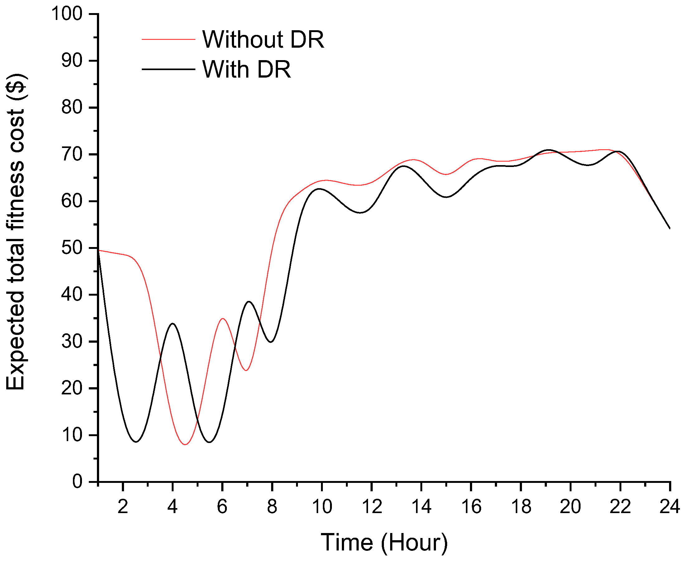
Figure 10b. The generation cost and emission of gases for the duration are shown in
Figure 11. The estimated cost comparison between the two scenarios is shown in
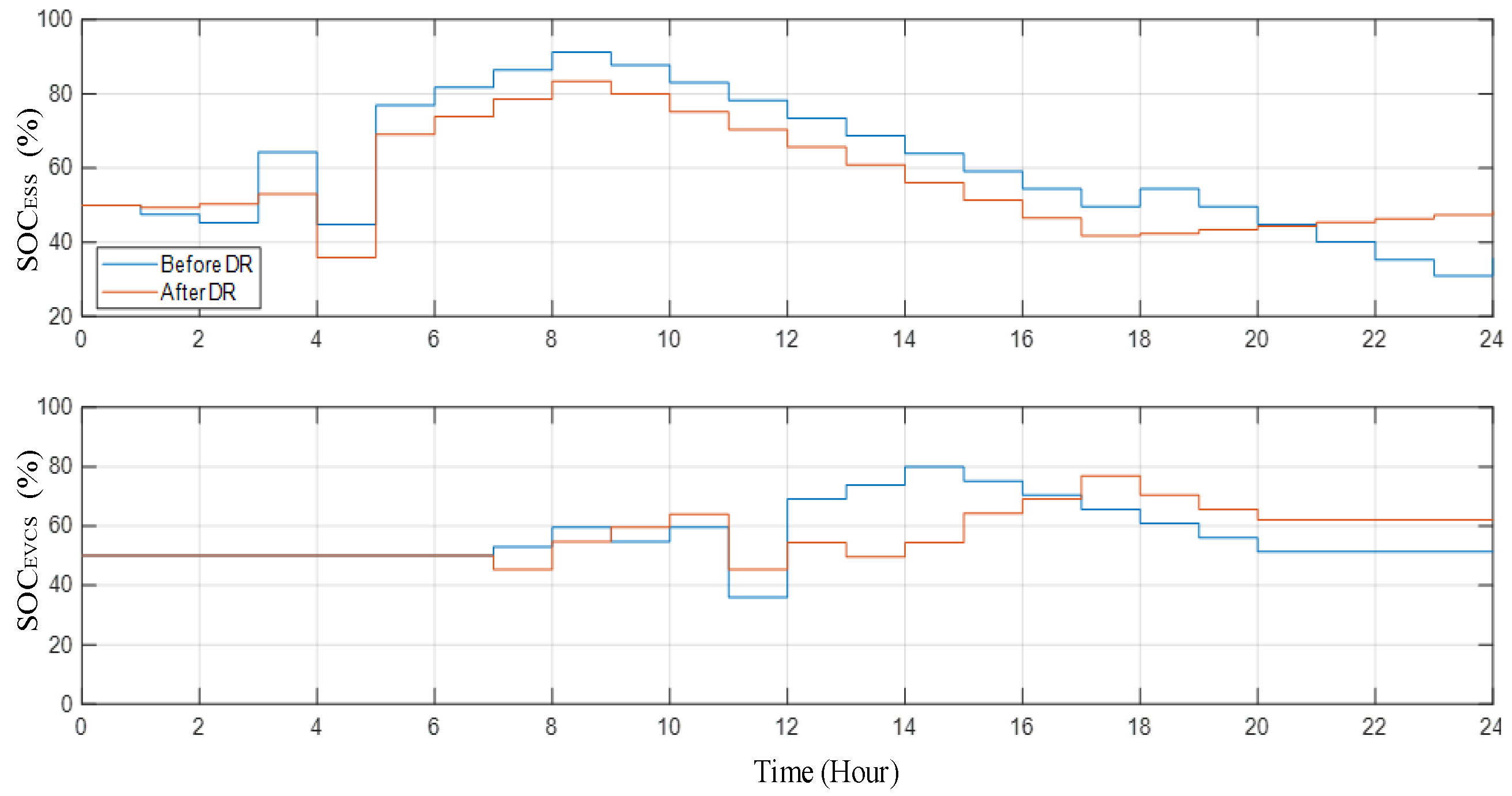
Figure 12. The state of charge for BESS and EVCS of both scenarios are shown to be within the parameter limits as in
Figure 13. The total fitness cost of the problem is USD 1224.15 with the overall cost of the system reduced by 18.91%, emission by 9.52%, and power loss by 9.65%. The change in demand for new pricing for this case is shown in
Figure 14.
4.3. Discussion and Validation
This section provides the analysis of the case studies and validation required for the proposed methodology. The grid-connected and islanded mode of energy management with demand response operations analysis is discussed in
Table 4. It is observed that with an increasing number of trails, the standard deviation is reducing but for optimality, 50 trails were run for the calculation of expected cost. In every case we discussed, the second scenario has reduced the operating cost and other objective parameters with respect to the previous scenario or the initial scenario. This shows the effectiveness of the strategy. Based on these results, the provided approach could be used to determine optimal operating costs reliably.
Hong’s 2 m method is performed for the proposed methodology as an uncertainty handling technique. In [
36,
39], the current test system is considered for the uncertainty of energy management. Hence the proposed method is compared with the above works and Monte Carlo simulation for the effective validation of the consistency in the approach.
Table 5. shows the comparison results with the proposed approach for the expected cost of the approach of the grid-connected scenario.
For Further analysis of the methodology, the author compared the proposed technique with popular algorithms such as particle swarm optimization (PSO) and firefly algorithm (FFA). The results of the comparison study are shown in
Table 6.
5. Conclusions
With demand response (DR) in the day ahead of energy management, the cost fitness of the optimal microgrid operations is improved. This article proposes day-ahead energy management through optimal demand shifting with suggestive incentive/penalty pricing at uncertainty. The pricing for the demand response program is developed so that the customers can choose the utilization of appliances with new pricing. The equipment’s controllability is updated to the user by the utility company providing him with an opportunity in making incentives. This strategy encourages the customers to manage their electricity billing while reducing the overall operating cost of the microgrid EMS. The uncertainties of forecasted data in renewable sources and load demand are handled by probability approximations using Hong’s 2 m PEM. The presented strategy is implemented on a typical microgrid over two cases of grid-connected and islanded mode. The results show that with the integration of load shifting-based DR strategy, there is an enhancement in objectives obtained when compared to the untampered scenario. The overall cost, power loss, and greenhouse emissions are reduced by 3.2%, 1.42%, and 1.76% in grid-connected cases and 10.5%, 9.2%, and 9.54% in islanding cases when compared. The effective management of the SOC in battery and charging stations shows the adaptivity of the system performance considering their degradation effects.
The proposed strategy could provide the operator with optimal DR to be operated with the uncertainties effect and how to tackle them. The practicality of the proposed method depends on the microgrid control center and the customer’s agreement to manage the utilities either manually through pricing or through intelligent utility control. The proposed method’s cost-effectiveness is compared with existing methodologies for validation and shows appreciable outcomes. To conclude, the proposed strategy benefits the control operator and the customer adopting the DR day-ahead energy management improves the intended objectives with the likely effect of uncertainties. The accuracy of the demand-side management could be improved with the inclusion of customer-side participation in defining the utilization of appliances and developing an estimated communication latency, which is considered for future extension.


