Understanding the Spatiotemporal Impacts of the Built Environment on Different Types of Metro Ridership: A Case Study in Wuhan, China

Abstract

As the backbone of passenger transportation in many large cities around the world, it is particularly important to explore the association between the built environment and metro ridership to promote the construction of smart cities. Although a large number of studies have explored the association between the built environment and metro ridership, they have rarely considered the spatial and temporal heterogeneity between metro ridership and the built environment. Based on metro smartcard data, this study used EM clustering to classify metro stations into five clusters based on the spatiotemporal travel characteristics of the ridership at metro stations. And the GBDT model in machine learning was used to explore the nonlinear association between the built environment and the ridership of different types of stations during four periods in a day (morning peak, noon, evening peak, and night). The results confirm the obvious spatial heterogeneity of the built environment’s impact on the ridership of different types of stations, as well as the obvious temporal heterogeneity of the impact on stations of the same type. In addition, almost all built environment factors have complex nonlinear effects on metro ridership and exhibit obvious threshold effects. It is worth noting that these findings will help the correct decisions be made in constructing land use measures that are compatible with metro functions in smart cities.

1. Introduction

Smart transportation is an important component of smart city construction. As a safe, punctual, and convenient urban transportation tool, the metro is the backbone of passenger transportation in many cities [1]. Big data can be used to analyze the micro mechanisms of residents’ metro travel behavior and spatial interaction, which play an important role in promoting the construction of smart cities. With the advancement of information technology, real-time metro smartcard data enables us to track metro passengers’ travel patterns [2,3]. Previous studies have found that metro ridership exhibits the characteristics of temporal and spatial change regularities, which are the result of residents’ time-varying travel demands and the differences in the surrounding areas of different metro stations [4,5]. Therefore, classifying inquiry metro ridership changes at different periods is not only helpful in understanding the spatiotemporal characteristics of residents’ metro travel but also in exploring the relationship between residents’ metro travel and land use in metro stations’ catchment area. This can further help planners and decision makers make planning decisions for optimizing land use in metro stations’ catchment areas in the construction of smart cities.

Different metro stations have differentiated metro ridership characteristics, which is due to the dual attribute features of metro stations [2,6]. On the one hand, metro stations are nodes in the metro network, allowing passengers to travel from one place to another [7]. On the other hand, metro stations are also places in the city. Under the influence of the TOD (transit-oriented development) strategy, the areas around metro stations usually adopt high-density mixed-development patterns and become key areas for human activity aggregation [8,9,10]. However, due to the differences in land use development around metro stations, metro ridership is significantly different across different metro stations [6,11,12]. For example, due to the commuting characteristics of the city’s work schedule, from 9 am to 5 pm, metro stations near residential areas may have larger inflow ridership during the morning peak and larger outflow ridership during the evening peak. Conversely, the trend in employment centers will be reversed. However, most of the existing studies have roughly analyzed ridership uniformly across all stations, and less attention has been paid to scaling the differences in metro ridership at different types of stations.

In addition, the built environment has long been considered an important factor affecting metro ridership [13,14,15]. Most existing studies have used the “5D” research framework to quantify the built environment [16,17,18,19], which measures the built environment according to five dimensions: density, diversity, design, transportation distance, and destination accessibility. While previous research has confirmed a high degree of correlation between the built environment and metro ridership, less attention has been paid to the possibility that the impact of the built environment on metro ridership may vary over time [1,20]. Furthermore, most previous studies on the relationship between the built environment and metro ridership have typically assumed a linear or generalized linear relationship, failing to reveal the nonlinear relationship between the two [21,22]. In summary, the nonlinear effects of the built environment on metro ridership at different periods have been rarely revealed.

To address the above issues, this study collected metro smartcard data in Wuhan, China. Firstly, using EM clustering analysis, metro stations were classified into different types. Then, the ridership was extracted for each metro station during four time periods, including morning peak, noon, evening peak, and night, and the GBDT model was applied using machine learning to explore the relative importance and nonlinear relationship between the built environment and ridership at different types of stations.

Therefore, this study contributes to the existing literature in both theory and practice. Firstly, it enriches the sparse existing literature on the relationship between the built environment and metro ridership by finely measuring the impact of the built environment on metro ridership at different types of stations and during different time periods. In addition, by exploring the relative importance and threshold effects of the built environment on metro ridership using the GBDT model of machine learning, it provides a reference for optimizing the built environment around metro stations in smart cities and formulating relevant policies.

The rest of this paper is arranged as follows. In Section 2, we review the literature related to the built environment and metro ridership. In Section 3, we introduce the study area and data source and present the metro station classification method and the machine learning model used in this study. In Section 4, we report the main findings of the study and conduct relevant discussions. In Section 5, we present the conclusions and policy implications of this study and point out future research directions.

2. Literature Review

Data used in traditional studies on residents’ travel behavior often rely on resident trip surveys [23,24,25], which have the advantage of capturing residents’ social attributes and can reflect their detailed travel characteristics. However, these data also have disadvantages, such as high survey cost, large time consumption, limited sample size, and most importantly, difficulty in acquiring real-time updates. With the significant development of real-time data collection technology through smartcard systems, smartcard data are widely used in travel behavior research due to their large sample size, high accuracy, and detailed spatiotemporal information [3,26,27,28]. Classifying real-time ridership in detail using smartcard data (SCD) can be helpful for understanding the relationship between the built environment and metro ridership at different types of stations.

Cluster analysis is an unsupervised classification method used to extract the most meaningful content [29]. As far as the functional classification of metro station is concerned, different classification results may be obtained from different perspectives. Some scholars classify metro stations’ functions from the perspective of the land use in the catchment area of a metro station. For instance, [30] classified New York metro stations into five categories, including commercial, highly mixed use, moderately mixed use, residential, and transfer residential, based on the intensity of commercial land use in the catchment areas of metro stations. Furthermore, some scholars classify metro station types in terms of the travel patterns of metro station passengers. For example, [29] classified Shanghai metro stations into six categories: employment stations, residential stations, mixed stations, mixed residential, mixed employment, and transportation hubs, based on the SCD of five consecutive weekdays. However, using land use to classify station types may not reflect the true travel patterns of metro ridership, since most cities have the characteristic of “city first, station later”, which causes some stations to have poor TOD guidance. Therefore, this study used SCD, which reflects the real travel patterns of metro passengers, to classify station types.

The built environment has long been proven to be an important factor affecting metro ridership, and the “5Ds” framework is often used to measure the built environment [13,14,16]. Density is an important indicator that affects metro ridership and is usually measured by resident population and the plot ratio, as high population concentration and spatial density may directly translate into metro ridership [31,32,33]. Diversity is mainly manifested in a mixture of land uses, which is more conducive to enhancing the attractiveness of the region and therefore promoting the demand for metro travel [4,22]. The number of street intersections is a commonly used indicator for measuring micro-level design, as more intersections indicate stronger road network connectivity, which enhances metro station accessibility and consequently promotes metro ridership growth [12,34,35]. However, some studies have found that the more street intersections, the longer the waiting time at traffic lights, which negatively affects metro ridership [11,36]. Travel distance is an indicator used to measure the convenience of metro stations and is usually represented by the number of bus stops in the catchment area of a metro station. Previous studies have found that the more bus stops, the more conducive an area is to bus–metro transfers, which further promotes metro ridership [36,37]. However, it has also been found that buses may divert metro ridership and in turn reduce metro usage [4]. Distance from the city center is usually used as an indicator of regional accessibility, and most studies show that stations closer to the city center have higher ridership due to the city center’s core role in employment and commerce [38,39]. In addition, the higher the number of daily travel destinations such as enterprises, shopping facilities, and living service facilities around metro stations, the more helpful it is for residents to choose metro travel [36,38,40,41]. Moreover, metro station characteristics also affect metro ridership. Previous studies have found that transfer stations, terminal stations, higher exit quantities, and higher betweenness centrality have a significant positive impact on metro ridership [11,20,36,42]. However, most existing studies consider all metro stations uniformly, with less subdivision of the relationship between different types of stations and the built environment in different catchment areas, during different periods, which causes the functional connection and temporal heterogeneity between the travel characteristics of different stations and land use to be largely ignored.

In addition, in previous studies on the relationship between the built environment and metro ridership, it is usually assumed that there is a linear or generalized linear relationship between the two, and linear regression models, Poisson regression models, or negative binomial regression models are commonly used to explore this relationship [1,21]. Although these studies have laid an effective foundation for understanding the relationship between the two, they cannot capture the nonlinear effects between them. Some recent studies have used supervised machine learning techniques to explore the relationship between the two and found that the impact of the built environment on metro ridership generally has complex nonlinear correlations [40,43]. For example, [22] used the GBDT model and found that intermediary centrality only has a positive promotion effect on metro ridership between 0 and 0.2; when the intermediary centrality further increases, it no longer has a positive promotion effect on metro ridership. Furthermore, [1] used the random forest model to reveal the impact of the built environment on metro ridership during morning peak, noon, and evening peak periods and found that there is a time heterogeneity between metro ridership and the built environment. However, the authors only examined ridership at all metro stations, so suggested that future research could focus on the correlation between the ridership of different types of stations and the built environment.

Existing studies have identified a number of research gaps in this field. Firstly, many previous studies have frequently treated all metro ridership as the dependent variable, neglecting the variations in travel behaviors contingent upon distinct metro station features. Particularly, there exist differences in ridership based on the functions of stations with different attributes and land use. Secondly, previous research has confirmed the significant nonlinear correlation between metro ridership and the built environment. However, due to the highly structured spatiotemporal regularities of residents’ travel activities and the marked temporal heterogeneity in their travel purposes, the temporal heterogeneity of the potential nonlinear relationship between the built environment and metro ridership has not been thoroughly discussed.

To address these gaps, our study undertook several key contributions. Firstly, leveraging a vast dataset of smartcard data, we effectively classified different types of metro stations through EM clustering, thereby revealing spatial disparities in travel characteristics among these distinct station types. Secondly, we extracted metro ridership from metro stations during four time periods: morning peak, noon, evening peak, and night. By employing the GBDT model, we investigated the relative importance and nonlinear effects of the built environment on metro ridership during these different time periods. This approach enables us to effectively identify the temporal heterogeneity in the nonlinear correlation between the built environment and metro ridership.

3. Research Design

3.1. Research Area

Wuhan, the largest city in central China, was the study area for this paper. Figure 1 shows the urban spatial structure of Wuhan, which is divided into the urban center within the Third Ring Road, and the Metropolitan Development Area (WMD) outside the Third Ring Road, where Wuhan has expanded in recent years. Due to the natural barrier of rivers and lakes, Wuhan has formed the three clusters of Hankou, Hanyang, and Wuchang, making it a typical polycentric city. In addition, the natural barriers have greatly restricted the organization of ground transportation in Wuhan, making metro travel popular among citizens. From 2010 to March 2021, the number of metro stations in Wuhan increased from 16 to 210 (transfer stations are not counted repeatedly), metro operating mileage increased from 28 km to 360 km, the share of the metro in public transportation also increased from 2% to 51%, and daily ridership has reached 3.1 million trips. Based on previous studies [6,16,44,45], this paper defines an 800 m buffer zone around the metro station as the station’s influence range, and the intersecting parts are processed using the Payson polygon technique.

3.2. Data and Variables

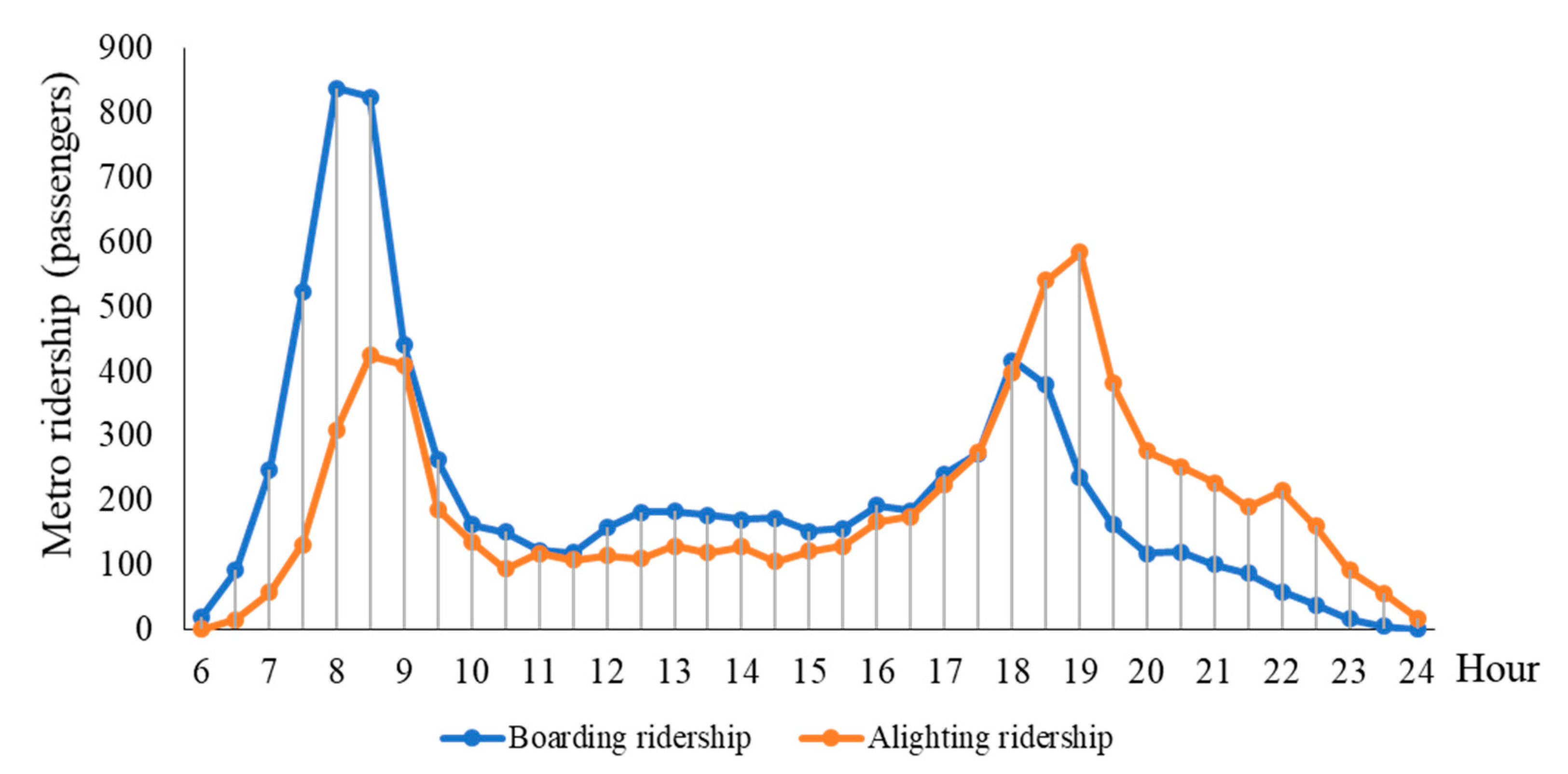
The data used in this paper include the smartcard data of 211 metro stations in Wuhan for five consecutive working days in March 2021, Wuhan point of interest (POI) data in 2021, building contour vector data, resident population data, and 2017 land use data in Wuhan. The smartcard data records the cardholder’s card number, entry and exit stations, swipe time, etc. Based on the card number and travel time information, we constructed travel OD chains from the origin to the destination of residents’ trips. After deleting some invalid data, a total of 9,392,605 travel OD chains were constructed, with a data validity rate of over 99%. Subsequently, the ridership for each metro station can be obtained by counting the number of passengers getting on and off at each station during each hour based on entry and exit time. The focus of this paper is the ridership on weekdays, so the ridership on non-workdays was not considered. Referring to the travel characteristics of residents’ daily life and work, we used the average ridership during four periods on workdays as the dependent variable, including the morning peak (7:00–9:00), noon (11:00–13:00), the evening peak (17:00–19:00), and night (21:00–23:00).

To examine the relationship between the built environment of a catchment area and metro ridership, we used the “5D” framework to construct the built environment variables [13]. Density included the resident population and the plot ratio of the catchment area; diversity was measured according to the land use mixture entropy score; the number of street intersections in the catchment area was used as a measure of design; the distance to public transport was represented by the number of bus stops in the catchment area; and accessibility to destinations was measured by the number of enterprises, shopping facilities, living service facilities, sports facilities, educational facilities, and medical facilities. In addition, considering the polycentric urban characteristics of Wuhan, the distances from the city center and sub-city center were selected to measure the regional accessibility of metro stations. Furthermore, this study also considered five factors affecting metro station characteristics: opening time, terminal station, transfer station, exit quantity, and betweenness centrality. Among them, the terminal station and transfer station are set as dummy variables corresponding to non-terminal and non-transfer stations. The specific indicator settings and definitions are shown in

Table 1. Description of the variables.

Variable	Variable Description	Mean	St.dev.
Metro ridership
7:00–9:00	Average metro ridership (people)	1230.91	968.50
11:00–13:00	Average metro ridership (people)	654.30	622.19
17:00–19:00	Average metro ridership (people)	1445.96	1391.61
21:00–23:00	Average metro ridership (people)	555.04	764.52
Built environment
Resident population	Population of residents in the catchment area (people)	20,308.59	21,381.45
Plot ratio	The plot ratio of the catchment area	2.21	1.66
Land use mixture	The land use mixture of the catchment area, calculated by the entropy method.	0.59	0.12
Number of intersections	Number of street intersection in the catchment area (count)	30.42	22.41
Number of bus stops	Number of bus stops in the catchment area (count)	26.74	14.76
Number of enterprises	Number of enterprises in the catchment area (count)	128.89	105.19
Number of shopping facilities	Number of shopping facilities in the catchment area (count)	604.48	821.94
Number of service facilities	Number of service facilities in the catchment area (count)	364.34	370.35
Number of medical facilities	Number of medical facilities in the catchment area (count)	69.09	64.19
Number of educational facilities	Number of educational facilities in the catchment area (count)	84.05	78.38
Number of sports facilities	Number of sports facilities in the catchment area (count)	58.98	75.22
Distance from the city center	Euclidean distance between the metro station and the city center (km)	11.39	7.28
Distance from the sub-city center	Euclidean distance between the metro station and the sub-city center (km)	6.75	5.79
Metro station features
Transfer station	Dummy variables, transfer station = 1, non-transfer station = 0	0.24	0.42
Terminal station	Dummy variables, terminal station = 1, non-terminal station = 0	0.05	0.22
Opening time	Metro station opening time (month)	86.92	46.74
Exit quantity	Number of exits in the metro station (count)	4.97	2.80
Betweenness centrality	Metro station betweenness centrality, computed by Pajek	0.07	0.06

.

3.3. Cluster Analysis

K-means clustering analysis is widely used due to its simplicity and efficiency when applied to the existing division method for metro station types [6]. However, K-means clustering analysis requires the pre-setting of the number of categories, and different category values can lead to significant differences in the results. In contrast, the EM clustering analysis does not require pre-set category values and divides categories based completely on objective data, which have more objective and stable characteristics [46]. Therefore, this study used EM clustering analysis to divide metro station types. Referring to the existing studies [46], EM clustering analysis has two steps and is obtained through alternate calculation:

Step 1: Calculate the expectation (E) to obtain the maximum likelihood estimate of the hidden variables.

Step 2: Maximize (M) the maximum likelihood value calculated in the first step to arrive at the value of the parameters.

The result of the M step is used in the next E step calculation, and this process is continuously iterated to continuously improve the initialization parameters through hidden variables until the parameters no longer change.

Under the framework of the EM algorithm, we chose the Gaussian mixture model (GMM) to solve the EM clustering. The GMM refers to a model with the following probability distribution:

$$P\left(y|\theta \right)=\sum _{k=1}^K{\alpha }_k\varnothing \left(y|{\theta }_k\right)$$

(1)

In the formula, $\sum _{k=1}^K{\alpha }_k=1$, and the probability density of the k-th Gaussian distribution is:

$$\varnothing \left(y|{\theta }_k\right)=\prod \frac{1}{\sqrt{2\pi {\theta }_k}}exp\left(-\frac{{\left(y-{\mu }_k\right)}^2}{2{\sigma }_k^2}\right)$$

(2)

where the model parameter ${\theta }_k=\left({\mu }_{k,}{\mu }_k\right)$.

3.4. GBDT Model

To better analyze the nonlinear impact of built environment features on metro ridership, this study constructed a gradient boosting decision tree (GBDT) model of machine learning. Compared with traditional regression models, GBDT does not predefine any form of correlation between independent variables and dependent variables and can effectively identify the nonlinear effects between them. Moreover, it can measure the relative importance of independent variables, which helps planners to determine intervention measures reasonably under limited conditions. In addition, GBDT adjusts the weight of the predictive variable by learning the data in stages, resulting in higher fitting accuracy than traditional regression models [40,43]. GBDT generates the predictive models in the form of model ensembles, which in this study are regression trees. The goal of this algorithm is to minimize the loss function. Regression trees can be defined as follows:

$$F\left(x\right)=\sum _{i=1}^m{f}_m\left(x\right)=\sum _{i=1}^m{\alpha }_{jm}I\left(x;{\epsilon }_m\right)$$

(3)

where the parameter ${\epsilon }_m$ represents the splitting position and the mean of the terminal node in each regression tree $I\left(x;{\epsilon }_m\right)$ and estimates ${\alpha }_{jm}$ by minimizing the loss function. The optimization process involves several iterative steps.

First, initialize the weak learner $f_0\left(x\right)$:

$$f_0\left(x\right)={\mathit{argmin}}_{\epsilon }\sum _{i=1}^{\mathrm{N}}L(y_i,\epsilon )$$

(4)

Second, for $m\left(m=\mathrm{1,2},3,...,M\right)$ iterations:

(a) Calculate the negative gradient (i.e., residual) ${\epsilon }_{im}$ for each sample $i\left(i=\mathrm{1,2},3,...,\mathrm{N}\right)$:

$${\epsilon }_{im}=-{\left[\frac{\partial L\left(y_i,f\left(x_i\right)\right)}{\partial f\left(x_i\right)}\right]}_{f\left(x\right)=f_{m-1}\left(x\right)}$$

(5)

(b) Fit a regression tree to the residual ${\epsilon }_{im}$ and obtain the leaf node region $A_{jm}$ of the m-th tree, where $j=\mathrm{1,2},3,...,J$., a tree composed of $J$ leaf nodes.

(c) Calculate the best fitting value ${\epsilon }_{im}$ for each leaf region $J$:

$${\epsilon }_{jm}=\mathit{arg}{\displaystyle \underset{\epsilon }{min}}\sum _{x_i\in A_{jm}}L\left(y_i,f_{m-1}\left(x_i\right)+\epsilon \right)$$

(6)

(d) Update the strong learner $f_m\left(x\right)$:

$$f_m\left(x\right)=f_{m-1}\left(x\right)+\sum _{j=1}^J{\epsilon }_{jm}I\left(x\in A_{jm}\right)$$

(7)

Finally, end the operation and obtain the final learner $f\left(x\right)=f_M\left(x\right)$.

In this study, we introduced a learning rate factor $\varphi \left(0<\varphi \le 1\right)$ to limit the residual learning results of each regression tree:

$$f_m\left(x\right)=f_{m-1}\left(x\right)+\varphi \cdot \sum _{j=1}^J{\epsilon }_{jm}I\left(x\in A_{jm}\right),0<\varphi \le 1$$

(8)

And we used the “gbm” package in the R platform to establish the GBDT model and export the relative importance of independent variables and the dependence graph of each variable.

4. Results and Discussion

4.1. Cluster Analysis Results

An EM clustering analysis was performed based on the “Mclust” package in RStudio, and the optimal number of categories was determined based on the Bayesian information criterion (BIC). According to Figure 2, the model converges best when the method is VEE and the number of clusters is five. The five specific components of the Mclust VEE (equal, ellipsoidal shape and orientation) model are shown in

Table 2. The five specific components of the Mclust VEE model.

1og-TikeTihood	n	df	BIC	ICL
−24,043.62	210	200	−49,309.22	−49,323.18

. Based on the changes in ridership over the time series and the peak-hour ridership indicators, we named the five categories of stations as mixed residential type, residential-oriented type, mixed employment type, employment-oriented type, and comprehensive type.

Cluster 1: Residential-oriented type, which includes 49 stations. Figure 3 shows the metro ridership characteristics of this cluster, which is characterized by high inbound ridership in the morning peak and high outbound ridership in the evening peak, with relatively low ridership in other periods. This type of station mainly provides travel services for commuters living near the station and is therefore classified as residential-oriented type.

Cluster 2: Mixed residential type, which includes 68 stations and is the largest cluster. Figure 4 shows the metro ridership characteristics of this cluster, which is similar to the residential-oriented type, with high inbound ridership in the morning peak and high outbound ridership in the evening peak. However, it also shows the characteristics of high outbound ridership in the morning peak and high inbound ridership in the evening peak, which accounts for a higher proportion than the residential-oriented type. This indicates that this type of station mainly provides travel services for commuters living near the station, while the region also has some commercial services such as employment or entertainment. Therefore, for Cluster 2, the corresponding stations should be classified as mixed residential type.

Cluster 3: Employment-oriented type, which includes 51 stations. Figure 5 shows the metro ridership characteristics of this cluster. In contrast to the residential-oriented type, the stations in this cluster are characterized by high outbound ridership in the morning peak and high inbound ridership in the evening peak. This type of station mainly provides travel services for commuters working near the station and is therefore classified as employment-oriented type.

Cluster 4: Mixed employment type, which includes 20 stations. Figure 6 shows the metro ridership characteristics of this cluster, which is also characterized by significant morning and evening dual peaks. But in contrast to the mixed residential type, it shows a higher number of outbound passengers in the morning peak and a higher number of inbound passengers in the evening peak. This indicates that this type of station mainly provides travel services for commuters working near the station, while there is also a certain proportion of residents who use the metro to commute. Therefore, for Cluster 4, the corresponding stations should be classified as mixed employment type.

Cluster 5: Comprehensive type, which includes 22 stations. Figure 7 shows the metro ridership characteristics of this cluster, which shows high outbound ridership in the morning peak and high inbound and outbound ridership in the evening peak, with the longest duration of inbound ridership in the evening peak, and also has a relatively large ridership in other periods. This indicates that the station is surrounded by a relatively rich variety of public service facilities, which is attractive to citizens in various periods. Therefore, the stations in this cluster are classified as comprehensive type.

Figure 8 shows the spatial distribution of stations in different clusters. It can be seen that Cluster 5 is mainly distributed on both sides of the Yangtze River and HanShui River in the urban center, while Cluster 3 and Cluster 4 are also mainly distributed within the Third Ring Road in the urban center. Cluster 1 and Cluster 2 gradually expand outward along the core area. Overall, comprehensive-type stations and employment-oriented-type stations are located in the urban center, while residential-oriented-type stations are mainly distributed in the outward areas along the urban center.

4.2. Relative Importance Analysis

The relative importance derived from the GBDT model reveals significant differences in the impact of the built environment on the metro ridership of different clusters in the four time periods, which are due to the spatiotemporal heterogeneity of residents’ travel behavior.

Specifically, for residential-oriented stations, it can be observed from Figure 9 that medical facilities, shopping facilities, distance from the sub-city center, and the number of enterprises are the most important indicators contributing to metro ridership in the four periods. Among them, the contribution of the distance from the sub-city center reached 16.14% in the evening peak, which is the highest indicator for residential-oriented stations in different periods. This is due to the fact that Wuhan is a typical polycentric city, and the sub-city centers have developed into the city’s employment, entertainment, and leisure centers and thus have a particularly significant impact on metro ridership during the evening peak. In addition, resident population has a relatively large impact on metro ridership at any period. This corresponds to the majority of previous research findings that the higher the resident population around metro stations, the more likely it is to be converted into metro ridership.

For mixed residential stations, it can be observed from Figure 10 that the number of shopping facilities, the number of enterprises, the distance from the city center, and the number of sports facilities are the most important indicators contributing to metro ridership in the four periods. Among them, the number of enterprises in the evening peak is the most important variable across the four periods, with a contribution rate of 33.42%. This is consistent with the typical nine-to-five work schedule in China. In addition, the number of sports facilities at night is the variable with the second highest contribution at 27.34%. This is because most people may choose to exercise at night due to work time constraints on weekdays, leading to higher metro ridership in stations near sports facilities at night. Moreover, the impact of distance from the city center on metro ridership is relatively large during any period. This corresponds to previous research results showing that metro stations located in the urban center usually have higher ridership [38].

For employment-oriented stations, it can be observed from Figure 11 that betweenness centrality, distance from the city center, the number of enterprises, and the number of sports facilities are the most important indicators contributing to metro ridership in the four periods. Consistent with our expectations, the number of enterprises has the greatest impact on metro ridership in the evening peak, reaching 31.53%, which is much higher than other variables. Similar to mixed residential stations, the number of sports facilities at night also has a relatively large impact on metro ridership, reaching 23.03. In addition, the impact of betweenness centrality on metro ridership during the morning peak also exceeded 20%. This is consistent with the research results of studies conducted on high-density cities such as Seoul, Shenzhen, and Shanghai [11,22,36], where the location of a metro station in the metro network is the most important factor affecting ridership. This is because better betweenness centrality of metro stations means higher accessibility to other metro stations.

For mixed employment stations, it can be observed from Figure 12 that resident population and the number of bus stops are the most important variables that contribute to metro ridership in the four periods. Among them, during the morning peak, evening peak, and night periods, both variables contribute more than 50% to the impact on metro ridership. This corresponds to previous research results, which show that resident population is a core factor promoting metro ridership [32,33], and the more bus stops around a metro station, the more favorable it is for bus–metro transfers, thereby promoting metro ridership growth. In addition, plot ratio is also an important factor affecting metro ridership in the four periods. This is consistent with the conclusions of most research on high-density cities [5,9], where a higher plot ratio means shorter potential travel distances, which is conducive to promoting metro travel.

For comprehensive stations, it can be observed from Figure 13 that betweenness centrality, resident population, land use mixture, and plot ratio are the most important variables contributing to metro ridership in the four periods. Unlike for the other four types of stations, land use mixture has a higher contribution to metro ridership at comprehensive stations, ranking third in importance in the morning peak, noon, and evening peak periods, with a contribution rate exceeding 10% during the morning and evening peaks. This indicates that mixed land use near comprehensive stations is more conducive to promoting metro ridership.

4.3. Nonlinear Analysis of the Built Environment on Metro Ridership

The GBDT model can explore the nonlinear relationship between the independent variable and the dependent variable, in addition to predicting the relative importance of the effects of independent variables on the dependent variable. The partial dependence plots derived from the GBDT model indicate that almost all built environment variables have nonlinear effects on metro ridership, and most variables exhibit distinct threshold effects. Moreover, the impact of each predictor on metro ridership varies significantly across different clusters and exhibits significant temporal heterogeneity across different periods. To facilitate comparison, based on the ranking of the relative importance of variables influencing metro ridership within each cluster, we selected the four variables with the highest cumulative relative importance across the four time periods of the day for comprehensive analysis.

Figure 14 shows the partial dependence plots for the four most important variables affecting metro ridership at residential-oriented stations. It can be observed that the number of medical facilities has a significant positive effect on metro ridership, with a clear threshold effect during the morning peak period. If the number of medical facilities in the catchment area increases from 0 to 22, during the morning peak, metro ridership will increase from 760 to 910. However, the promotional effect on metro ridership becomes imperceptible when the number of medical facilities further increases. Shopping facilities also have a positive impact on metro ridership, but unlike medical facilities, the impact of shopping facilities on metro ridership is more pronounced during the noon period. Distance from the sub-city center has a negative impact on metro ridership, which is consistent with most existing research [38]. As a typical polycentric city, the sub-city center also serves as the employment and leisure center, which usually has a larger ridership. From the changes in the four periods, it can be found that when the distance from the sub-city center increases from 3 km to 10 km, metro ridership decreases sharply. When the distance from the sub-city center further increases to 16 km, ridership continues to decline to the lowest point during the noon period, while ridership remains relatively stable during the other three periods. This finding has profound practical implications for the location selection of sub-city centers in polycentric cities. The number of enterprises has a positive impact on metro ridership, especially during the night period. Specifically, when the number of enterprises in the catchment area exceeds 220, metro ridership increases sharply. This is in line with our expectations, as in areas where enterprises are concentrated, road congestion at night may still be severe, and the metro, which is not affected by surface transportation, is more attractive to commuters.

Figure 15 shows the partial dependence plots for the four most important variables affecting metro ridership at mixed residential stations. It can be observed that the number of shopping facilities has a positive effect on metro ridership, similar to that of residential-oriented stations. However, for mixed residential stations, the impact on metro ridership is more significant during the morning peak period. The impact of the number of enterprises on metro ridership exhibits a significant difference between the morning peak and other periods. During the morning peak, the number of enterprises has a negative impact on metro ridership, as commuters usually travel from their residences to their workplaces in the morning, resulting in less metro ridership in areas with more enterprises. In other periods, however, residents usually travel from their workplace to other areas, resulting in a positive impact on metro ridership. The impact of the number of sports facilities on metro ridership is similar to that of the number of enterprises, exhibiting a negative impact during the morning peak but a positive impact in other periods. Distance from the city center also has a significant negative impact on metro ridership, with a much higher effect during the morning peak than in the other three periods, and reflects a more pronounced threshold effect. During the morning peak period, metro ridership sharply decreases from 2500 to 0 as the distance from the city center gradually increases from 3 km to 20 km.

Figure 16 shows the partial dependence plots for the four most important variables affecting metro ridership at employment-oriented stations. It can be observed that betweenness centrality overall has a significant positive effect on metro ridership, which is consistent with most research results [22]. Metro stations located in network centers usually have higher accessibility, and the areas around these stations are more likely to be favored for urban development as sub-city centers, thus contributing to an increase in metro ridership. Similar to the results of other clusters, distance from the city center has a significant negative impact on metro ridership. The number of enterprises exhibits a negative impact during the morning peak and at noon and a positive impact during the evening peak and at night, which is consistent with China’s commuting patterns of going out early and coming home late. The number of sports facilities has a significant positive impact during the morning peak and at night but a negative impact at noon and during the evening peak for employment-oriented stations. This differs somewhat from the impact on mixed residential stations, but it is consistent with the lifestyle of many employed people in China, who exercise in the morning or evening due to work time constraints.

Figure 17 shows the partial dependence plots for the four most important variables affecting metro ridership at mixed employment stations. It can be observed that resident population has a strong impact on metro ridership, which is consistent with most of the existing literature [9,32]. In addition, it has a more significant impact on metro ridership during the morning and evening peaks, as there is usually greater demand for travel during these times. Moreover, there is a clear threshold effect of resident population on metro ridership during the noon and night periods. When the population in a catchment area exceeds 6000, the marginal effect becomes difficult to discern. As the number of bus stops in the catchment area increases from 5 to 10, metro ridership increases significantly in all four periods. However, interpreting these results requires caution, as while the higher number of bus stops in the catchment area, the more useable the station is for bus–metro transfers, it may also have a diversion effect on metro ridership. In Wuhan, as metro lines are opened for operation, bus routes are usually adjusted simultaneously to promote bus–metro integration, which is an important factor that makes the number of bus stops positively promote metro ridership at different times. Plot ratio has a positive promotional effect on metro ridership, while the distance from the city center has a negative impact, which is consistent with the results observed in other clusters.

Figure 18 shows the partial dependence plots for the four most important variables affecting metro ridership at comprehensive stations. It can be observed that betweenness centrality has a negative impact on metro ridership, which is inconsistent with most research results [11,36]. This is because comprehensive stations have a large number of passengers, and stations with high betweenness centrality have higher ridership, usually more than 1000 passengers per hour, while the maximum passenger capacity of Wuhan’s metro trains is mostly between 1000 and 2000 passengers. To avoid congestion and waiting, people may choose other modes of transportation. During holidays, Wuhan has also implemented measures such as flow control and temporary closure of metro stations at core comprehensive stations to avoid safety hazards. The resident population has a significant positive impact on metro ridership at comprehensive stations, which is similar to the results of other clusters. The number of street intersections has a positive promotional effect on metro ridership, which corresponds to most existing research [34]. The more street intersections, the higher the accessibility of metro stations, which is conducive to promoting metro travel. Especially near comprehensive stations in Wuhan, many areas are usually closed to vehicles and are pedestrian only, which further promotes the growth of metro ridership. Land use mixture has a positive promotional effect on metro ridership and has a clear threshold effect. When the land use mixture is less than 0.58, the impact on metro ridership is minimal. However, when the land use mixture further increases to around 0.7, metro ridership increases significantly in all four periods. When the land use mixture further increases, it no longer has an impact on metro ridership. We believe that identifying the classifications of the inflection point of land use mixture on metro ridership is particularly important, especially for promoting TOD planning and practices in smart city construction.

In summary, all built environment variables exert significant nonlinear influences on metro ridership. These effects exhibit notable variations across different types of stations and during different time periods, while also displaying pronounced threshold effects. Moreover, these threshold effects manifest distinct nonlinear characteristics across different types of metro stations and during different time periods. Despite the transit-oriented development (TOD) principle advocating for high-density and mixed-use development around metro stations, our study reveals that excessive development and population concentration could potentially exacerbate traffic congestion and environmental degradation, consequently diminishing residents’ willingness to use the metro. Furthermore, mixed land use does not universally enhance metro ridership across all station types; it prominently enhances metro ridership only for comprehensive stations. Additionally, analogous trends are observed in other built environment variables, with relative importance and threshold effects differing significantly across different types of stations.

5. Conclusions

The purpose of this study was to better understand the spatiotemporal correlation between the built environment and resident metro travel through in-depth data mining. To achieve this, the study used smartcard data from the Wuhan metro system in China, combined with multi-source big data such as land use data and POI data, and applied an EM clustering model to divide metro stations into five clusters based on spatiotemporal ridership characteristics of metro travel. The study then uses the GBDT model of machine learning to explore the nonlinear relationship between metro ridership at different types of stations and built environment factors during different times of the day. The study results fill an important research gap and provide some interesting and meaningful findings.

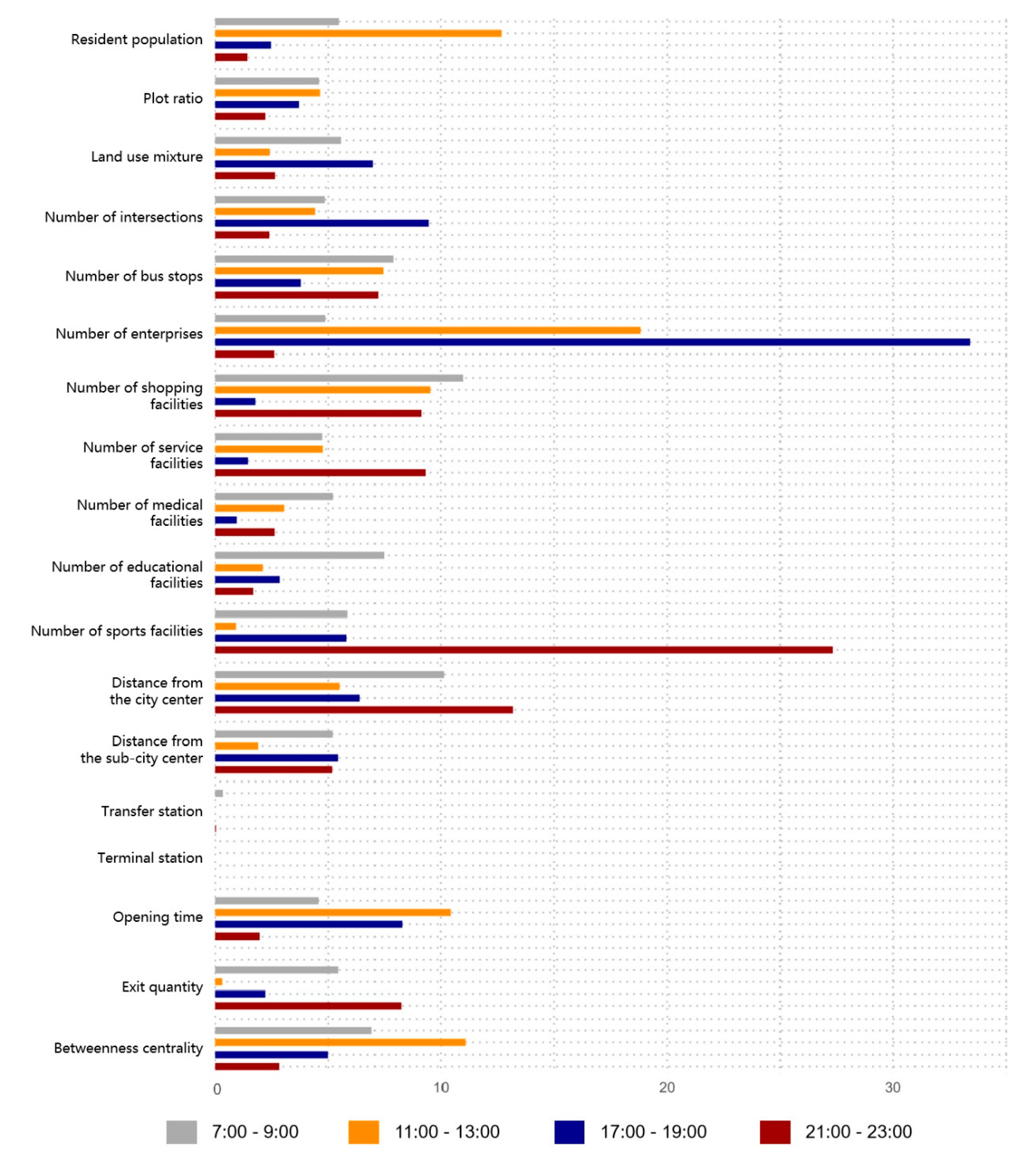
Firstly, based on the detailed travel spatiotemporal characteristics of each station, the EM clustering model was used to divide metro stations into five clusters: residential-oriented stations, mixed residential stations, employment-oriented stations, mixed employment stations, and comprehensive stations. Each type of station has different travel spatiotemporal characteristics, which provides a foundation for understanding the relationship between resident travel characteristics and urban land use functions. Although this study used Wuhan as an example, this classification method is also applicable to other cities. Secondly, the study confirms that the relative importance of the built environment on ridership at different types of stations varies significantly. For residential-oriented stations, the distance from the sub-city center is the most significant factor influencing ridership, while the number of enterprises plays the most crucial role in employment-oriented station ridership. Betweenness centrality emerges as the most pivotal variable impacting metro ridership in comprehensive stations, while the number of enterprises, as well as the distance from the sub-city center, are the most vital factors respectively influencing mixed residential and mixed employment station ridership. Additionally, the relative importance of these factors exhibits distinct disparities across stations of the same type during different time periods. For instance, in the case of residential-oriented stations, the number of medical facilities, number of shopping facilities, distance from the sub-city center, and number of enterprises were the most significant factors during the morning peak, noon, evening peak, and night periods, respectively. It is worth noting that resident population has a strong impact on metro ridership at all stations during different periods, which further confirms that high-density TOD development patterns are conducive to promoting public transportation travel [9,22]. 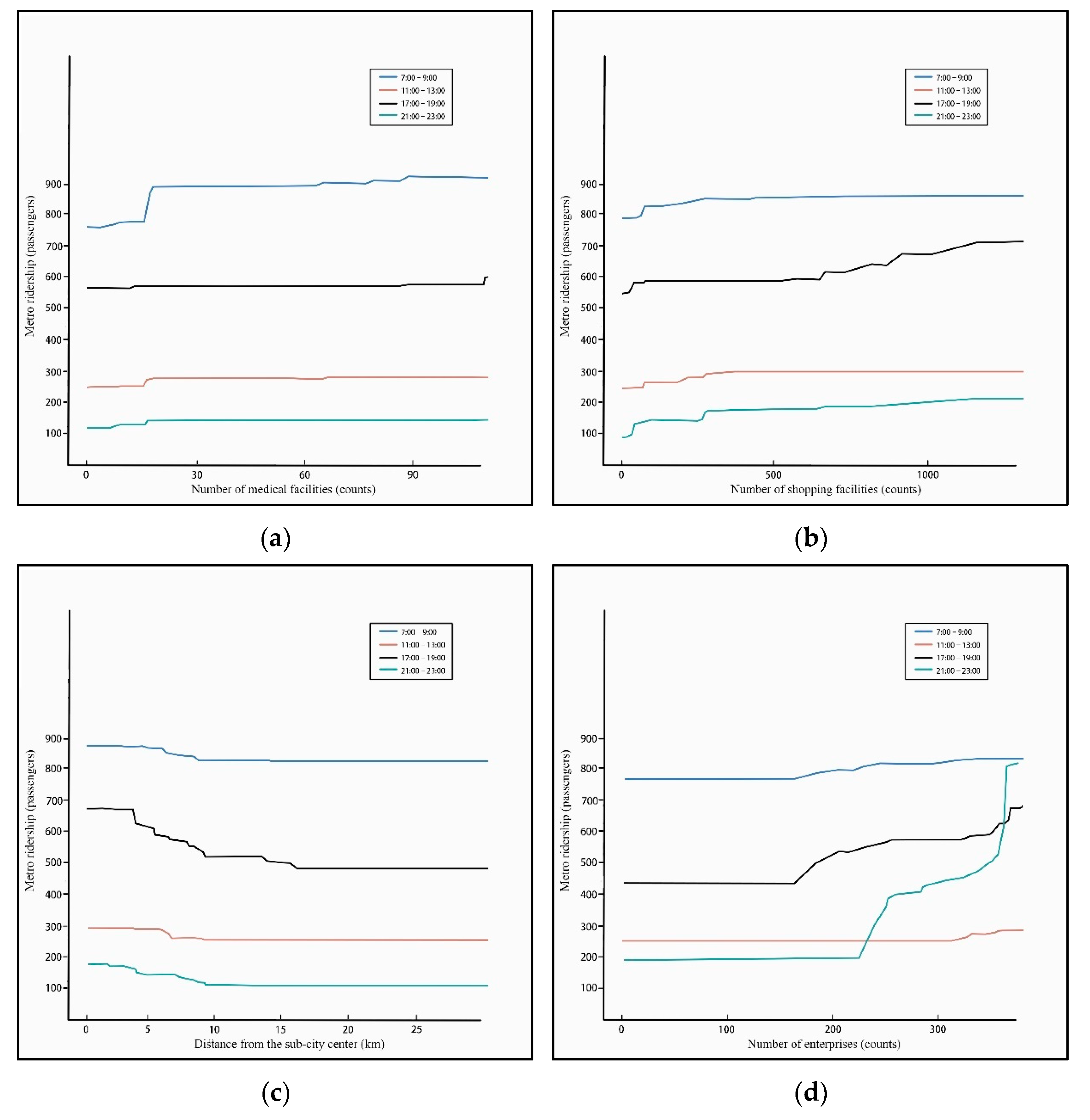However, land use mixture only has a significant impact on ridership in comprehensive stations, which may explain the difference between previous research results regarding the impact of land use mixture on metro ridership [4,21], as mixed land use may not be effective in all areas. Third, most built environment variables have complex nonlinear effects on metro ridership at any time and in any cluster of stations and show significant threshold effects.

These findings have important planning and policy implications for urban planning and related departments regarding the optimization of land use at metro stations in the construction of smart cities. Firstly, the relative importance of the built environment to the metro ridership of different types of stations provides a reference for the priority order of built environment intervention in different regions. Therefore, urban planning authorities should formulate distinct land use development measures based on the diverse station types and characteristics of residents’ travel behaviors. For residential-oriented stations, the optimization of public service facilities catering to daily needs, such as medical and shopping facilities, should be prioritized. In the case of employment-oriented stations and mixed residential stations, there should be a concerted effort to attract enterprises to within the vicinity of these metro stations while enhancing the accessibility of these enterprises to the metro stations. As for comprehensive stations and mixed employment stations, promoting population concentration through compact development proves most effective in bolstering metro ridership. Moreover, prevailing transit-oriented development (TOD) paradigms emphasize the significance of high-density and mixed-use development. However, our research demonstrates that population density exerts a pivotal influence across all station types, while land use mixture only contributes very significantly to comprehensive stations. This suggests that a compact and intensive development model contributes to enhancing metro ridership across all station types, but mixed land use significantly enhances ridership only for comprehensive stations. Thirdly, the threshold effect of the built environment on metro ridership provides an impact range for optimizing the built environment. For example, for comprehensive stations, when the land use mixture reaches 0.58, the metro ridership reaches an inflection point and gradually increases. However, when the land use mixture further grows to 0.7, it no longer exhibits a significant promoting effect. This serves as a reminder to urban planners that planning interventions below the threshold or beyond the threshold may not yield effective outcomes. It is essential to devise land use optimization measures within an effective influence range. Fourthly, the impact of the built environment on metro ridership has significant spatiotemporal heterogeneity, which may remind urban planning and transportation management departments to pay attention to the characteristics of metro travel demand and the job–housing balance. The different ridership of different types of stations at different times and their different associations with the built environment remind us that transportation planning and urban functional layout should not be simply based on daily ridership. Spatial organization and transportation planning should be carried out according to the travel demands of urban residents during different periods. Especially for the layout of urban employment centers and residential areas, avoiding long-distance commuting and job–housing unbalance is key.

By dividing metro stations into clusters based on their spatiotemporal travel characteristics and exploring the nonlinear relationship between ridership and the built environment at different times for different clusters, this study reveals the relationship between residents’ metro travel characteristics and urban land use, which will help optimize land use around metro stations in smart city construction and policy formulation. However, this study still has some shortcomings that are worth exploring further in future research. First, this study defines an 800 m buffer zone around the metro station as the station’s influence range based on previous research [16,44], but different types of metro stations may have different influence ranges. In the future, a more reasonable catchment area should be defined based on the classification results of metro stations and combined with residents’ travel survey data. In addition, this study did not consider the impact of residents’ social attributes on the ridership of different types of metro stations. This should be remedied in the future by increasing the use of questionnaire surveys, which will help to formulate more refined measures. Finally, the conclusions of this study cannot be generalized to other cities, especially those with medium- and low-density oriented development. Therefore, more cases of different development-oriented cities should be added to further research to verify the accuracy of this study’s results.

References

1. Yang, L.; Yu, B.; Liang, Y.; Lu, Y.; Li, W. Time-Varying and Non-Linear Associations between Metro Ridership and the Built Environment. Tunn. Undergr. Space Technol. 2023, 132, 104931. [Google Scholar] [CrossRef]
2. Amini Pishro, A.; Yang, Q.; Zhang, S.; Amini Pishro, M.; Zhang, Z.; Zhao, Y.; Postel, V.; Huang, D.; Li, W.Y. Node, Place, Ridership, and Time Model for Rail-Transit Stations: A Case Study. Sci. Rep. 2022, 12, 16120. [Google Scholar] [CrossRef]
3. Yong, J.; Zheng, L.; Mao, X.; Tang, X.; Gao, A.; Liu, W. Mining Metro Commuting Mobility Patterns Using Massive Smart Card Data. Phys. A Stat. Mech. Its Appl. 2021, 584, 126351. [Google Scholar] [CrossRef]
4. Li, S.; Lyu, D.; Liu, X.; Tan, Z.; Gao, F.; Huang, G.; Wu, Z. The Varying Patterns of Rail Transit Ridership and Their Relationships with Fine-Scale Built Environment Factors: Big Data Analytics from Guangzhou. Cities 2020, 99, 102580. [Google Scholar] [CrossRef]
5. Yang, H.; Ruan, Z.; Li, W.; Zhu, H.; Zhao, J.; Peng, J. The Impact of Built Environment Factors on Elderly People’s Mobility Characteristics by Metro System Considering Spatial Heterogeneity. ISPRS Int. J. Geoinf. 2022, 11, 315. [Google Scholar] [CrossRef]
6. Gan, Z.; Yang, M.; Feng, T.; Timmermans, H. Understanding Urban Mobility Patterns from a Spatiotemporal Perspective: Daily Ridership Profiles of Metro Stations. Transportation 2020, 47, 315–336. [Google Scholar] [CrossRef]
7. Peng, J.; Cui, C.; Qi, J.; Ruan, Z.; Dai, Q.; Yang, H. The Evolvement of Rail Transit Network Structure and Impact on Travel Characteristics: A Case Study of Wuhan. ISPRS Int. J. Geoinf. 2021, 10, 789. [Google Scholar] [CrossRef]
8. Ibraeva, A.; Van Wee, B.; Correia, G.H.d.A.; Pais Antunes, A. Longitudinal Macro-Analysis of Car-Use Changes Resulting from a TOD-Type Project: The Case of Metro Do Porto (Portugal). J. Transp. Geogr. 2021, 92, 103036. [Google Scholar] [CrossRef]
9. Su, S.; Zhao, C.; Zhou, H.; Li, B.; Kang, M. Unraveling the Relative Contribution of TOD Structural Factors to Metro Ridership: A Novel Localized Modeling Approach with Implications on Spatial Planning. J. Transp. Geogr. 2022, 100, 103308. [Google Scholar] [CrossRef]
10. Huang, J.; Chen, S.; Xu, Q.; Chen, Y.; Hu, J. Relationship between Built Environment Characteristics of TOD and Subway Ridership: A Causal Inference and Regression Analysis of the Beijing Subway. J. Rail Transp. Plan. Manag. 2022, 24, 100341. [Google Scholar] [CrossRef]
11. Jun, M.J.; Choi, K.; Jeong, J.E.; Kwon, K.H.; Kim, H.J. Land Use Characteristics of Subway Catchment Areas and Their Influence on Subway Ridership in Seoul. J. Transp. Geogr. 2015, 48, 30–40. [Google Scholar] [CrossRef]
12. Zhang, M. The Role of Land Use in Travel Mode Choice: Evidence from Boston and Hong Kong. J. Am. Plan. Assoc. 2004, 70, 344–360. [Google Scholar] [CrossRef]
13. Ewing, R.; Cervero, R. Travel and the Built Environment. J. Am. Plan. Assoc. 2010, 76, 265–294. [Google Scholar] [CrossRef]
14. Zhang, Y.; Zhao, P.; Lin, J.J. Exploring Shopping Travel Behavior of Millennials in Beijing: Impacts of Built Environment, Life Stages, and Subjective Preferences. Transp. Res. Part. A Policy Pract. 2021, 147, 49–60. [Google Scholar] [CrossRef]
15. Guo, J.Y.; Chen, C. The Built Environment and Travel Behavior: Making the Connection. Transportation 2007, 34, 529–533. [Google Scholar] [CrossRef]
16. Yang, H.; Lu, Y.; Wang, J.; Zheng, Y.; Ruan, Z.; Peng, J. Understanding Post-Pandemic Metro Commuting Ridership by Considering the Built Environment: A Quasi-Natural Experiment in Wuhan, China. Sustain. Cities Soc. 2023, 96, 104626. [Google Scholar] [CrossRef]
17. Xiao, W.; Wei, Y.D.; Wu, Y. Neighborhood, Built Environment and Resilience in Transportation during the COVID-19 Pandemic. Transp. Res. D Transp. Environ. 2022, 110, 103428. [Google Scholar] [CrossRef]
18. Cheng, L.; Chen, X.; Yang, S.; Cao, Z.; De Vos, J.; Witlox, F. Active Travel for Active Ageing in China: The Role of Built Environment. J. Transp. Geogr. 2019, 76, 142–152. [Google Scholar] [CrossRef]
19. Feng, J. The Influence of Built Environment on Travel Behavior of the Elderly in Urban China. Transp. Res. D Transp. Environ. 2017, 52, 619–633. [Google Scholar] [CrossRef]
20. Gan, Z.; Yang, M.; Feng, T.; Timmermans, H.J.P. Examining the Relationship between Built Environment and Metro Ridership at Station-to-Station Level. Transp. Res. D Transp. Environ. 2020, 82, 102332. [Google Scholar] [CrossRef]
21. Ding, C.; Cao, X.; Liu, C. How Does the Station-Area Built Environment Influence Metrorail Ridership? Using Gradient Boosting Decision Trees to Identify Non-Linear Thresholds. J. Transp. Geogr. 2019, 77, 70–78. [Google Scholar] [CrossRef]
22. Shao, Q.; Zhang, W.; Cao, X.; Yang, J.; Yin, J. Threshold and Moderating Effects of Land Use on Metro Ridership in Shenzhen: Implications for TOD Planning. J. Transp. Geogr. 2020, 89, 102878. [Google Scholar] [CrossRef]
23. Nasri, A.; Carrion, C.; Zhang, L.; Baghaei, B. Using Propensity Score Matching Technique to Address Self-Selection in Transit-Oriented Development (TOD) Areas. Transportation 2020, 47, 359–371. [Google Scholar] [CrossRef]
24. Van de Coevering, P.; Maat, K.; van Wee, B. Residential Self-Selection, Reverse Causality and Residential Dissonance. A Latent Class Transition Model of Interactions between the Built Environment, Travel Attitudes and Travel Behavior. Transp. Res. Part. A Policy Pract. 2018, 118, 466–479. [Google Scholar] [CrossRef]
25. Chen, F.; Wu, J.; Chen, X.; Nielsen, C.P. Disentangling the Impacts of the Built Environment and Residential Self-Selection on Travel Behavior: An Empirical Study in the Context of Diversified Housing Types. Cities 2021, 116, 103285. [Google Scholar] [CrossRef]
26. Gong, Y.; Lin, Y.; Duan, Z. Exploring the Spatiotemporal Structure of Dynamic Urban Space Using Metro Smart Card Records. Comput. Environ. Urban. Syst. 2017, 64, 169–183. [Google Scholar] [CrossRef]
27. Chen, E.; Ye, Z.; Wang, C.; Zhang, W. Discovering the Spatio-Temporal Impacts of Built Environment on Metro Ridership Using Smart Card Data. Cities 2019, 95, 102359. [Google Scholar] [CrossRef]
28. Chu, K.K.A. Two-Year Worth of Smart Card Transaction Data—Extracting Longitudinal Observations for the Understanding of Travel Behaviour. Proceedings of the Transportation Research Procedia. 2015, 11, 365–380. [Google Scholar] [CrossRef]
29. Jiao, H.; Huang, S.; Zhou, Y. Understanding the Land Use Function of Station Areas Based on Spatiotemporal Similarity in Rail Transit Ridership: A Case Study in Shanghai, China. J. Transp. Geogr. 2023, 109, 103568. [Google Scholar] [CrossRef]
30. Chen, C.; Chen, J.; Barry, J. Diurnal Pattern of Transit Ridership: A Case Study of the New York City Subway System. J. Transp. Geogr. 2009, 17, 176–186. [Google Scholar] [CrossRef]
31. Zhao, P. The Impact of the Built Environment on Individual Workers’ Commuting Behavior in Beijing. Int. J. Sustain. Transp. 2013, 7, 389–415. [Google Scholar] [CrossRef]
32. Yin, C.; Cao, J.; Sun, B. Examining Non-Linear Associations between Population Density and Waist-Hip Ratio: An Application of Gradient Boosting Decision Trees. Cities 2020, 107, 102899. [Google Scholar] [CrossRef]
33. Sun, G.; Lau, C.Y. Go-along with Older People to Public Transport in High-Density Cities: Understanding the Concerns and Walking Barriers through Their Lens. J. Transp. Health 2021, 21, 101072. [Google Scholar] [CrossRef]
34. Durning, M.; Townsend, C. Direct Ridership Model of Rail Rapid Transit Systems in Canada. Transp. Res. Rec. 2015, 2537, 96–102. [Google Scholar] [CrossRef]
35. Sun, B.; Ermagun, A.; Dan, B. Built Environmental Impacts on Commuting Mode Choice and Distance: Evidence from Shanghai. Transp. Res. D Transp. Environ. 2017, 52, 441–453. [Google Scholar] [CrossRef]
36. An, D.; Tong, X.; Liu, K.; Chan, E.H.W. Understanding the Impact of Built Environment on Metro Ridership Using Open Source in Shanghai. Cities 2019, 93, 177–187. [Google Scholar] [CrossRef]
37. Kuby, M.; Barranda, A.; Upchurch, C. Factors Influencing Light-Rail Station Boardings in the United States. Transp. Res. Part. A Policy Pract. 2004, 38, 223–247. [Google Scholar] [CrossRef]
38. Zhao, J.; Deng, W.; Song, Y.; Zhu, Y. What Influences Metro Station Ridership in China? Insights from Nanjing. Cities 2013, 35, 114–124. [Google Scholar] [CrossRef]
39. Zhao, J.; Deng, W.; Song, Y.; Zhu, Y. Analysis of Metro Ridership at Station Level and Station-to-Station Level in Nanjing: An Approach Based on Direct Demand Models. Transportation 2014, 41, 133–155. [Google Scholar] [CrossRef]
40. Du, Q.; Zhou, Y.; Huang, Y.; Wang, Y.; Bai, L. Spatiotemporal Exploration of the Non-Linear Impacts of Accessibility on Metro Ridership. J. Transp. Geogr. 2022, 102, 103380. [Google Scholar] [CrossRef]
41. Choi, J.; Lee, Y.J.; Kim, T.; Sohn, K. An Analysis of Metro Ridership at the Station-to-Station Level in Seoul. Transportation 2012, 39, 705–722. [Google Scholar] [CrossRef]
42. Sohn, K.; Shim, H. Factors Generating Boardings at Metro Stations in the Seoul Metropolitan Area. Cities 2010, 27, 358–368. [Google Scholar] [CrossRef]
43. Tao, T.; Wang, J.; Cao, X. Exploring the Non-Linear Associations between Spatial Attributes and Walking Distance to Transit. J. Transp. Geogr. 2020, 82, 102560. [Google Scholar] [CrossRef]
44. Guo, Y.; Yang, L.; Lu, Y.; Zhao, R. Dockless Bike-Sharing as a Feeder Mode of Metro Commute? The Role of the Feeder-Related Built Environment: Analytical Framework and Empirical Evidence. Sustain. Cities Soc. 2021, 65, 102594. [Google Scholar] [CrossRef]
45. Liu, B.; Xu, Y.; Guo, S.; Yu, M.; Lin, Z.; Yang, H. Examining the Nonlinear Impacts of Origin-Destination Built Environment on Metro Ridership at Station-to-Station Level. ISPRS Int. J. Geoinf. 2023, 12, 59. [Google Scholar] [CrossRef]
46. Hou, W.; Chen, Y.; Liu, H.; Xiao, F.; Liu, C.; Wang, D. Reconstructing Three-Dimensional Geological Structures by the Multiple-Point Statistics Method Coupled with a Deep Neural Network: A Case Study of a Metro Station in Guangzhou, China. Tunn. Undergr. Space Technol. 2023, 136, 105089. [Google Scholar] [CrossRef]
Figure 1. Research area.
Smartcities 06 00105 g001
Figure 2. Bayesian information criterion curves for different methods and numbers of clusters. Note: The bold blue line is the clustering result of the VEE method.
Smartcities 06 00105 g002
Figure 3. The spatiotemporal characteristics of Cluster 1 station travel.
Smartcities 06 00105 g003
Figure 4. The spatiotemporal characteristics of Cluster 2 station travel.
Smartcities 06 00105 g004
Figure 5. The spatiotemporal characteristics of Cluster 3 station travel.
Smartcities 06 00105 g005
Figure 6. The spatiotemporal characteristics of Cluster 4 station travel.
Smartcities 06 00105 g006
Figure 7. The spatiotemporal characteristics of Cluster 5 station travel.
Smartcities 06 00105 g007
Figure 8. Spatial distribution of stations in different clusters.
Smartcities 06 00105 g008
Figure 9. Relative importance of variables for residential-oriented stations.
Smartcities 06 00105 g009
Figure 10. Relative importance of variables for mixed residential stations.
Smartcities 06 00105 g010
Figure 11. Relative importance of variables for employment-oriented stations.
Smartcities 06 00105 g011
Figure 12. Relative importance of variables for mixed employment stations.
Smartcities 06 00105 g012
Figure 13. Relative importance of variables for comprehensive stations.
Smartcities 06 00105 g013
Figure 14. Partial dependence plot for residential-oriented stations. (a) Number of medical facilities. (b) Number of shopping facilities. (c) Distance from the sub-city center. (d) Number of enterprises.
Smartcities 06 00105 g014
Figure 15. Partial dependence plot for mixed residential stations. (a) Number of shopping facilities. (b) Number of enterprises. (c) Number of sports facilities. (d) Distance from the city center.
Smartcities 06 00105 g015
Figure 16. Partial dependence plot for employment-oriented stations. (a) Betweenness centrality. (b) Distance from the city center. (c) Number of enterprises. (d) Number of sports facilities.
Smartcities 06 00105 g016
Figure 17. Partial dependence plot for mixed employment stations. (a) Resident population. (b) Number of bus stops. (c) Plot ratio. (d) Distance from the city center.
Smartcities 06 00105 g017
Figure 18. Partial dependence plot for comprehensive stations. (a) Betweenness centrality. (b) Resident population. (c) Number of intersections. (d) Land use mixture.
Smartcities 06 00105 g018