Effectiveness of the Fuzzy Logic Control to Manage the Microclimate Inside a Smart Insulated Greenhouse

Abstract

Agricultural greenhouses incorporate intricate systems to regulate the internal climate. Among the crucial climatic variables, indoor temperature and humidity take precedence in establishing an optimal environment for plant production and growth. The present research emphasizes the efficacy of employing intelligent control systems in the automation of the indoor climate for smart insulated greenhouses (SIGs), utilizing a fuzzy logic controller (FLC). This paper proposes the use of an FLC to reduce the energy consumption of a greenhouse. In the first step, a thermodynamic model is presented and experimentally validated based on thermal heat exchanges between the indoor and outdoor climatic variables. The outcomes show the effectiveness of the proposed model in controlling indoor air temperature and relative humidity with a low error percentage. Secondly, several fuzzy logic control models have been developed to regulate the indoor temperature and humidity for cold and hot periods. The results show the good performance of the proposed FLC model as highlighted by the statistical analysis. In fact, the root mean squared error (RMSE) is very small and equal to 0.69% for temperature and 0.23% for humidity, whereas the efficiency factor (EF) of the fuzzy logic control is equal to 99.35% for temperature control and 99.86% for humidity control.

1. Introduction

A greenhouse is a purposefully constructed enclosure, typically made of materials such as glass or transparent polymers, designed to create and maintain an environment suitable for plant cultivation. The main purpose of a greenhouse is to capture and retain solar energy, establishing a controlled climate within the structure. This controlled environment enables continuous plant growth throughout the year, providing favorable conditions even for species that may face challenges thriving in the local climate under natural conditions. For these reasons, the development of a smart greenhouse requires a comprehensive study, encompassing various steps. These steps include the modeling of the system, the validation and performance assessment of the model, and the implementation of intelligent control to ensure the effective management of the indoor climate.

Greenhouse climate systems are complex, with numerous interconnected variables such as temperature, humidity, light intensity, CO₂ levels, and airflow. Modeling and controlling these variables require sophisticated algorithms and sensors, which can be challenging to implement and maintain. Many researchers focus on modeling and developing a microclimate for agricultural greenhouses. In particular, the authors in [1] study the different models of the greenhouse and present an overview of the current state of greenhouse modeling, while other authors deal with the parameter identification of a greenhouse model, by means of process optimization and multi-model integration [2]. A greenhouse model based on a deep neural network is presented in [3,4], whereas Ref. [5] proposes a dynamic model based on the assessment and investigation. Other authors [6] use this model for heat transfer to improve the procedure for directly predicting the air temperature in agricultural greenhouses. The physical model [7,8,9] is an important issue for greenhouses because it can help define the reference for a favorable indoor climate. A new model to simulate the distribution of the radiation inside an agrivoltaic greenhouse was developed in [10], while a novel greenhouse energy model aimed at predicting the year-round indoor microclimate of commercial greenhouses was presented in [11]. The impact of some variables—air temperature and relative humidity inside the greenhouses—have a crucial role in the modeling of the greenhouse [12,13,14]. In particular, the relative humidity is considered in a deep learning model to predict evapotranspiration and moisture control in tomato greenhouses [15]. Reviews on the role of humidity and temperature in controlling the indoor climate of a dynamic agricultural greenhouse in tomato cultivation are available [16,17]. The heat exchanges between the indoor and outdoor environments of the greenhouse system are also crucial for correctly modeling the system, as studied in [18], whereas studies on the heat exchange of the canopy in the greenhouses with heating and cooling systems are discussed in [19,20]. In [21], the authors suggest a method for predicting the canopy temperature and heat flux, based on the leaf area index of bell peppers in a greenhouse environment, whereas a correlation between the heat temperature of the ground and the canopy thermal behavior for cooling and heating of the greenhouse is discussed in [22]. This methodology has been applied to a real glass greenhouse in Romania. Since environmental conditions are crucial for the optimal conditions in any greenhouse, environment sensors [23] and the management of environmental data [24,25,26] constitute further research areas for greenhouse management. Several issues can arise from the accuracy of models and the smart control of the internal climates of greenhouse systems, such as the complexity and variability of the greenhouse environment, making it difficult to maintain consistent climate conditions. In this context, some literature studies focus on different modeling methods for greenhouses. Ref. [27] reviewed the application of artificial neural networks in the greenhouse technology model. Ref. [28] proposed a neural network method to predict the accuracy of a process-based greenhouse climate–tomato production model by using particle filtering and deep learning. Moreover, Ref. [29] built a Deep Elman RNN model based on climate and actuator variables and stated that the obtained model would be used for control tasks.

Addressing the issues of energy consumption and promoting sustainable practices in greenhouse cultivation necessitate a combination of technological innovation, operational best practices, and continuous research aimed at enhancing control algorithms and systems. In this context, the control of the greenhouse environment is intricate, characterized by its non-linear nature and multiple inputs and outputs (MIMOs). Several control algorithms, such as proportional–integral–derivative (PID), fuzzy logic (FL), neural networks, and hybrid approaches, have been utilized to manage greenhouse systems [30]. The implementation of the strategy control in the greenhouse model offers an efficient technique for maintaining the desired microclimate. Moreover, the optimization efficiency of greenhouses is significantly enhanced thanks to the control strategy. Many literature research works have addressed the control of the greenhouse system. For example, the authors in [31,32,33] present an adaptive control supply to manage the indoor climate of the greenhouse with a cooling and fogging system. Some researchers have developed control systems using physical and dynamic models of greenhouses with neural networks [4,34,35], focusing on the intelligent monitoring of the microclimate to guarantee an optimal set-point. They encompass the management of temperature, humidity [36], irrigation [37], and ventilation [38]. Intelligent control and energy optimization in controlled environment agriculture via nonlinear model predictive control (MPC) of the semi-closed greenhouse was developed by [39]. The feedback/feedforward control method can be combined with MPC or PID to improve the performance [40]; Ref. [41] developed an application of nonlinear adaptive control for managing the temperature of Chinese solar greenhouses. These control methods are presented to optimize indoor greenhouse climates.

On the other hand, intelligent algorithms make use of artificial intelligence techniques and results useful in the absence of a mathematical model. However, they require large sets of data for the model training. The FLC is a control method used to solve the non-linear greenhouse system, and the literature focuses on the efficacy of fuzzy logic to manage the indoor climate of the greenhouse [42]. Nevertheless, FLC stands out as the suitable choice for application in nonlinear systems like greenhouses [43]; references [17,44] developed a comprehensive monitoring and control system for temperature and humidity in industrial greenhouses based on fuzzy logic. Additionally, the development of a prototype for the control and monitoring system of a smart greenhouse using fuzzy logic methods is described in [45]. Instead, reference [46] proposed an intelligent control strategy that describes the design of a greenhouse system using fuzzy logic to manage climate, humidity, and lighting conditions. An advantage of FLC is that it operates effectively without fixing the limits of the controlled system. This approach exhibits strong robustness and adaptability, making it well-received by the operators. Traditional fuzzy logic systems often rely on static membership functions and rule sets, which may not adapt well to changing environmental conditions or varying crop requirements. To address the gaps in precision and adaptability of the fuzzy control strategy in the literature, this study focuses on adaptive smart fuzzy systems where membership functions can dynamically adjust based on real-time data. This approach aims to enhance the precision and adaptability of greenhouse control systems, making them more responsive to varying conditions. Additionally, this study explores the development of membership functions and rules that prioritize energy-efficient operations, optimizing heating and cooling to reduce energy consumption while maintaining optimal growing conditions. It also aims to address scalability issues by the tailored membership functions for each major input, which can lead to smoother transitions in the output signal, reducing the sensitivity to small changes in the input. Thus, it is highly suitable for managing intricate systems like SIGs. The efficacy of the greenhouse models with and without control is studied in the literature by using some known statistical indexes such as RMSE, TSSE, MAPE, and EF. For the performance assessment of a greenhouse model, it is advisable to consider a combination of these metrics to gain a comprehensive understanding of the model’s strengths and weaknesses in different aspects of accuracy, efficiency, and relative error. Additionally, the metric choice may depend on the specific goals and requirements of the greenhouse control and management system.

This work has a twofold target: to optimize the dynamic and physical model of a smart greenhouse and to evaluate the effectiveness of the FLC-based control strategy to ensure a favorable microclimate for crops within the greenhouse. Initially, the proposed modeling of various greenhouse components, coupled with the data acquisition system from sensors for continuous environmental monitoring, is experimentally validated to solve the complexity of the greenhouse. Moreover, a smart FLC is developed and optimized to regulate the indoor climate of the greenhouse to reduce energy consumption and optimal climate variability. The performance of the fuzzy strategy is evaluated through statistical analysis to assess its efficacy during both cold and hot periods. The paper proposes two different types of FLCs. The first one is based only on two indoor variables (air temperature and humidity), whereas the second one is based on four variables (indoor and outdoor air temperature and humidity). This paper is organized as follows. Section 2 provides a comprehensive overview of the greenhouse, the modeling approach adopted for the greenhouse, and the definitions of several statistical metrics. Moving on to Section 3, detailed descriptions of an experimental greenhouse and measurement devices are presented. This section also discusses the thermal modeling of the insulated greenhouse. Subsequently, Section 4 delves into the depiction of the control strategy, and two types of FLC (FLC-I and FLC-II) are defined. The results and discussion will form the focal point of Section 5. Section 6 presents the conclusions of the paper.

2. Methodology

2.1. Improvement Techniques of a Smart Insulated Greenhouse (SIG)

This paper offers a significant contribution to the automation of agricultural greenhouses, enhancing production efficiency in several ways. Firstly, it focuses on improving greenhouse infrastructure through effective insulation. Secondly, it concentrates on developing several heat exchange mechanisms within the greenhouse to achieve an optimal microclimate, which is a crucial factor in streamlining the control strategy. Thirdly, it proposes a control strategy by implementing intelligent FLCs based on the data sensor of the indoor and outdoor climatic parameters, efficiently managing the microclimate. This comprehensive approach is designed to optimize the performance control strategy of the greenhouse, ensuring optimal growing conditions, and facilitating the control of environmental parameters. The main points are as follows:

• The geometry of a greenhouse involves its structure and operation to achieve energy efficiency, maximize plant growth, and minimize the environmental impact. Greenhouse modeling can benefit from various techniques and strategies to achieve these goals. One optimization technique for modeling greenhouses is insulating the foundation to prevent heat loss through the floor of the greenhouse, in order to provide thermal insulation and support for the greenhouse structure.
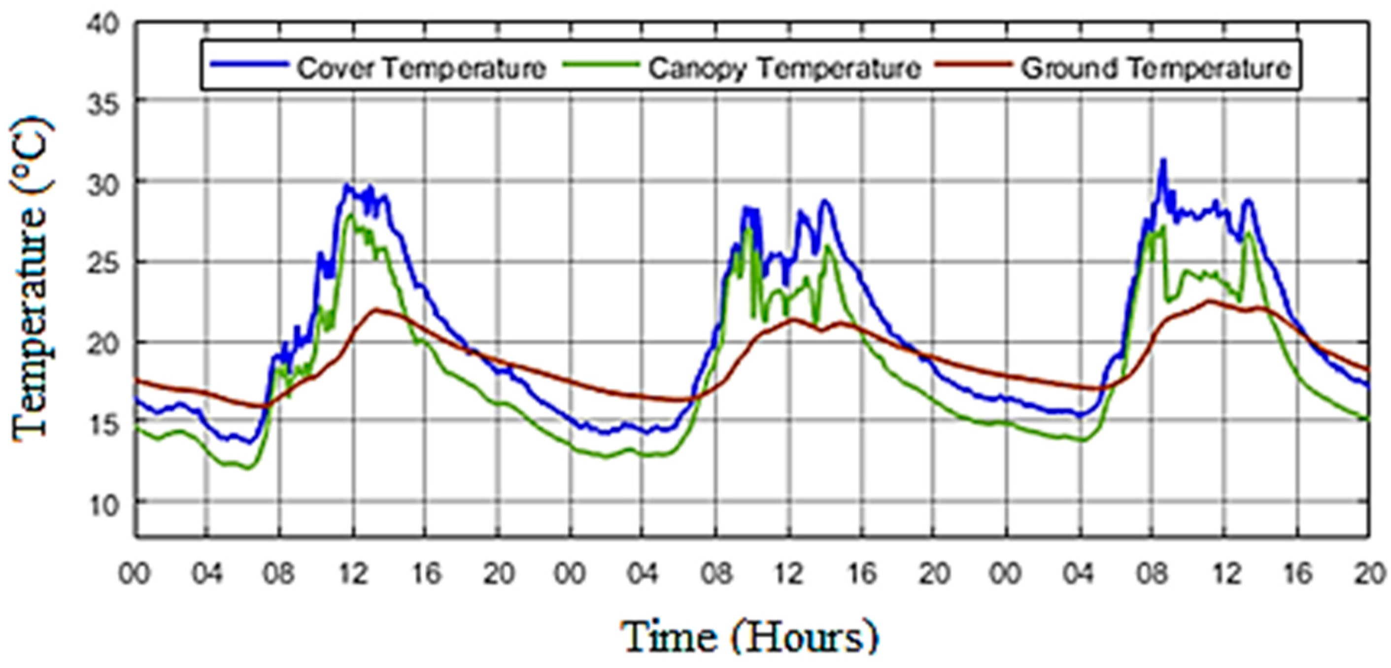
• Heat transfer mechanisms within the proposed SIG have been studied to create an ideal indoor environment for cultivation. Specifically, the influence of the canopy temperature, cover, and ground temperature in a greenhouse system can have a significant impact on the indoor climate and the growth of plants. These factors are included in a mathematical model of the SIG to create an ideal greenhouse environment involving a careful balance to meet the specific needs of the plants.
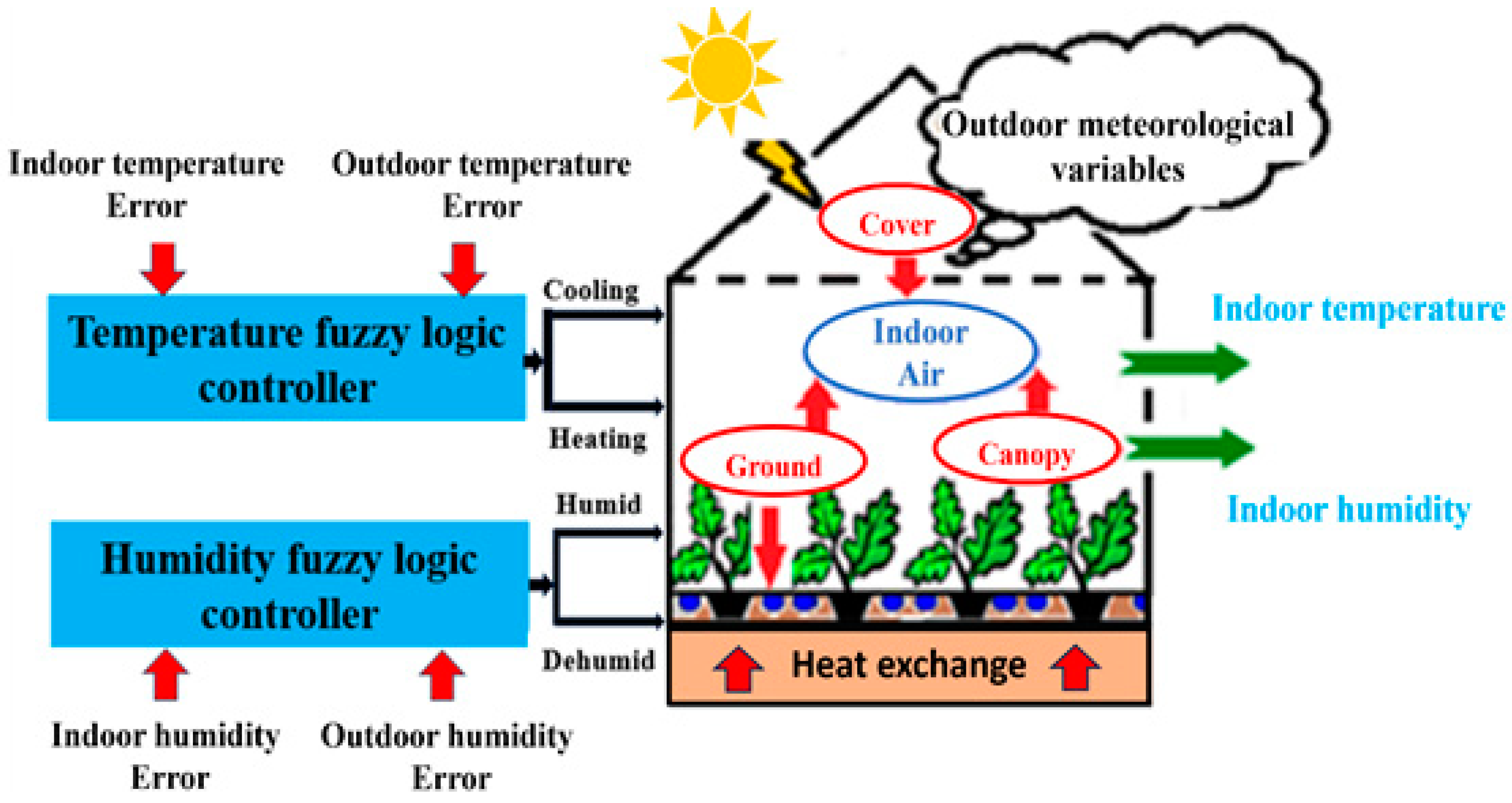
• The control approach hinges on implementing instrumentation for monitoring the thermal parameters of the SIG, utilizing indoor and outdoor sensors. The indoor climate control is achieved through intelligent FLCs that operate actuators, taking into account the climatic fluctuations and their impact on the automation technology (cooling and heating system).
• Figure 1 presents the SIG under test and it is constituted by the following parts:
  • Two FLCs (blue blocks) to control the temperature and humidity of the SIG;
  • A greenhouse system (pentagon block) that contains the heat exchanges between the indoor air and outdoor variables (shown by the green arrows).

2.2. Statistical Analysis

The utilization of various performance metrics in this study reflects a comprehensive evaluation of the insulated greenhouse model and the applied control strategy. Each metric provides a different perspective on the accuracy and efficiency of the model and control strategy. The performance metrics used in this paper are as follows:

• Root mean square error (RMSE), which calculates the square root of the mean of the squared differences between predicted and actual values. It represents the standard deviation of the errors, providing an indication of how spread out these errors are.
• Total sum of squared error (TSSE), which is the sum of the squared errors between predicted and actual values. It provides a comprehensive measure of the overall error in the model’s predictions.
• Mean absolute percentage error (MAPE), which measures the average percentage difference between predicted and actual values. It provides insight into the accuracy of predictions and is particularly useful for understanding the magnitude of errors.
• Efficiency factor (EF), which is a metric that assesses the performance of a model by comparing the predicted and observed variances. It is expressed as a percentage and is particularly useful for evaluating the efficiency of models that predict dynamic processes, such as changes in temperature and humidity.

The determination of the model exhibiting the highest accuracy is based on achieving the lowest MAPE, RMSE, and TSSE values, and the highest EF value. This multi-metric approach ensures a thorough evaluation, considering not only the magnitude of errors but also their distribution and the efficiency of the model in capturing the dynamic changes. They are calculated on the basis of the acquired data series to compare the predicted values, F_i, to the measured values, M_i, with a sample number n equal to 426 (see

Table 1. Accuracy of statistical analysis.

Name	Equation	Abbreviation and Unit
Root mean squared error	$\mathrm{R}\mathrm{M}\mathrm{S}\mathrm{E}=\sqrt{\frac{\sum _{\mathrm{i}=1}^{\mathrm{n}}{\left({\mathrm{M}}_{\mathrm{i}}-{\mathrm{F}}_{\mathrm{i}}\right)}^2}{\mathrm{n}}}$	RMSE
Total sum of squared error	$\mathrm{T}\mathrm{S}\mathrm{S}\mathrm{E}={\displaystyle \sum _{\mathrm{i}=1}^{\mathrm{n}}}{\left({\mathrm{M}}_{\mathrm{i}}-{\mathrm{F}}_{\mathrm{i}}\right)}^2$	TSSE
Mean absolute percentage error	$\mathrm{M}\mathrm{A}\mathrm{P}\mathrm{E}=\frac{1}{\mathrm{n}}{\displaystyle \sum _{\mathrm{j}=1}^{\mathrm{n}}}\left|\frac{{\mathrm{M}}_{\mathrm{i}}-{\mathrm{F}}_{\mathrm{i}}}{{\mathrm{M}}_{\mathrm{i}}}\right|\ast 100$	MAPE
Model efficiency factor	$\mathrm{E}\mathrm{F}=\frac{\sum _{\mathrm{i}=1}^{\mathrm{n}}{\left({\mathrm{M}}_{\mathrm{i}}-\overline{\mathrm{M}}\right)}^2-\sum _{\mathrm{i}=1}^{\mathrm{n}}{\left({\mathrm{M}}_{\mathrm{i}}-{\mathrm{F}}_{\mathrm{i}}\right)}^2}{\sum _{\mathrm{i}=1}^{\mathrm{n}}{\left({\mathrm{M}}_{\mathrm{i}}-\overline{\mathrm{M}}\right)}^2}$	EF

, where $\overline{M}$ is the average value of all M_i) [47,48]. Sometimes, the RMSE value is calculated in percentage form, such as $\frac{RMSE}{\overline{M}}·100$.

The relationships between the statistical analyses are the following:

• RMSE and TSSE measure error magnitude, but RMSE normalizes by the number of observations.
• MAPE and TSSE focus on the difference between predicted and observed values, but MAPE does not directly involve squared errors and provides a relative measure of accuracy.
• EF is concerned with how well the model performs compared to a baseline model, whereas a lower TSSE in the model compared to the baseline results in a higher EF.

3. Materials and Modeling

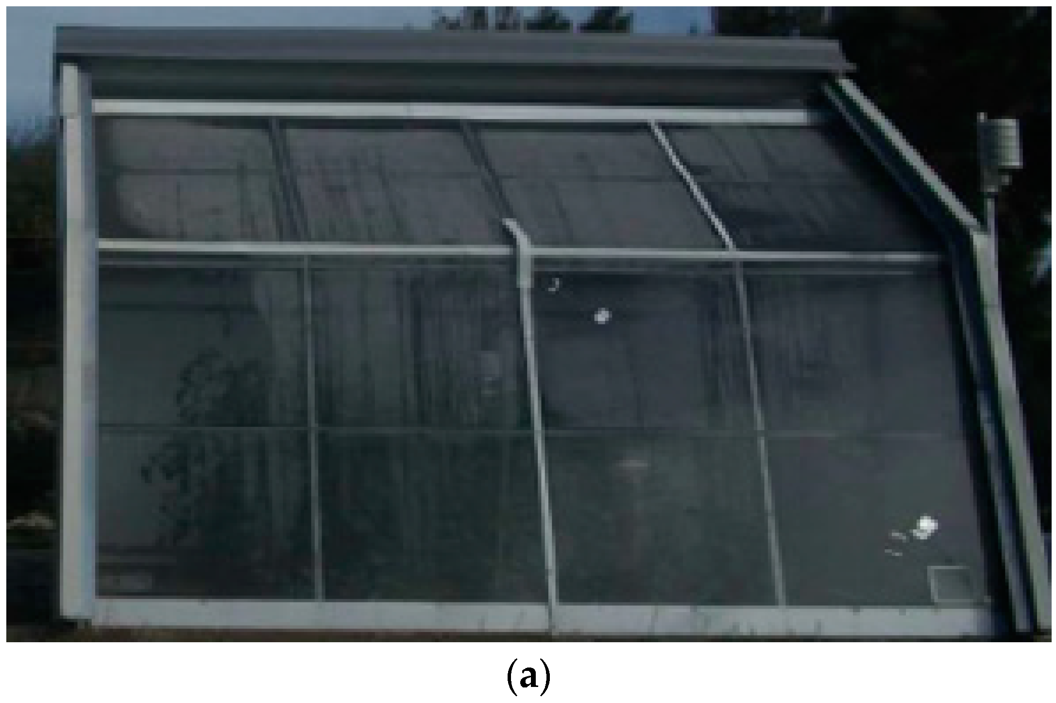
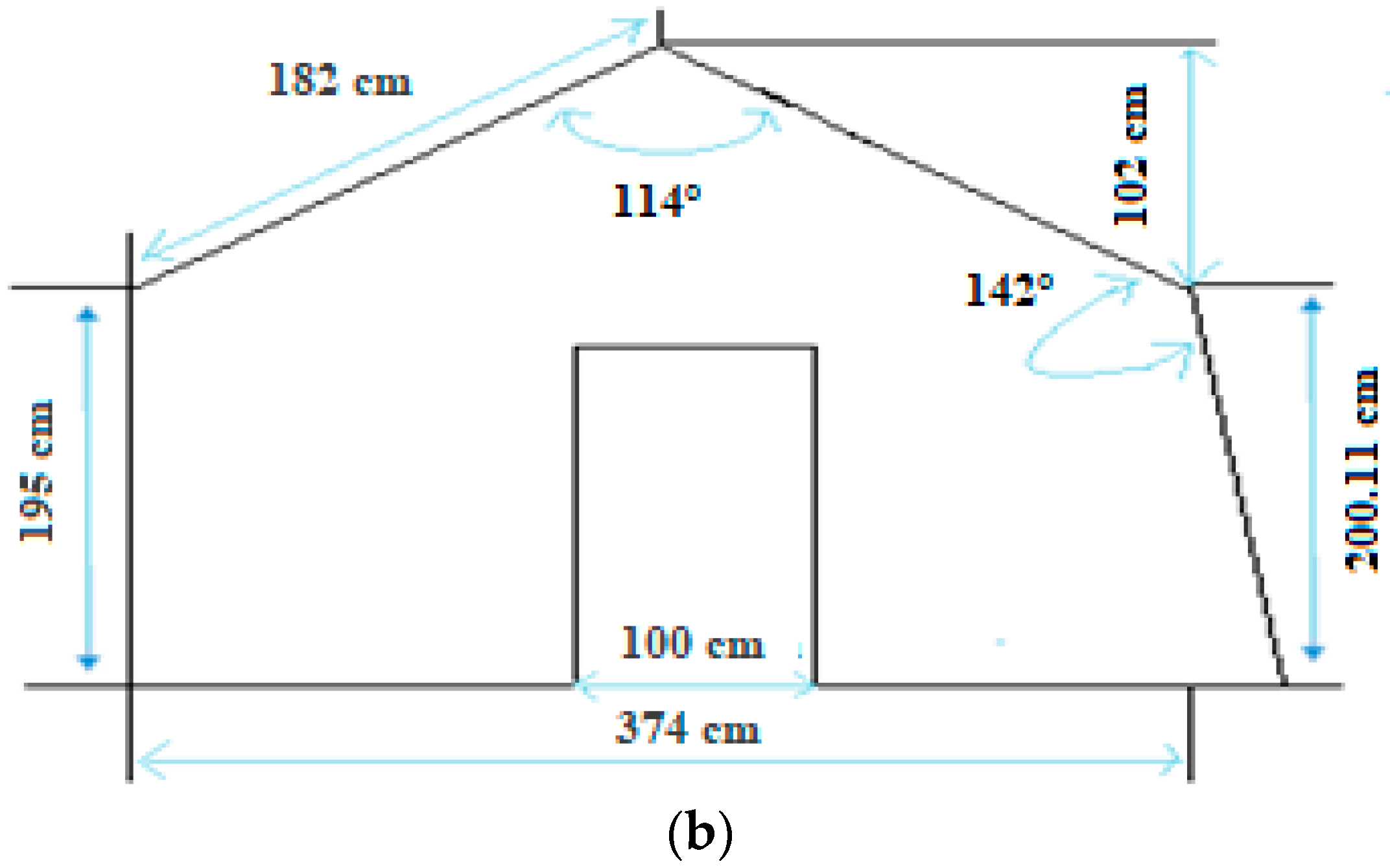
3.1. Description of the Experimental Greenhouse

In this research, an experimental well-insulated greenhouse (Figure 2a) was designed for the cultivation of tomatoes, a commonly practiced method in Tunisia, especially in the northern region of Tunis (located at latitude 36°41′46.68″ N). This design incorporates a 0.4 m-thick sandwich panel for the side walls and a 0.6 m-thick panel for the north-facing roof, while the south-facing walls and roof are covered with 0.003 m-thick Plexiglas panels. The detailed greenhouse specifications, as depicted in Figure 2b, indicate that it covers a ground area of 14.8 m², with dimensions of about 4 m in length, 3.74 m in width, and 3.02 m in height. The glazing material chosen for this greenhouse is glass, whose thermal characteristics are reported in

Table 2. Characteristics of greenhouse glass cover [47].

Characteristics	Values (%)
Transmissivity for solar radiation	0.85
Reflectivity for solar radiation	0.10
Reflectivity for thermal radiation	0.10
Emissivity	0.89
Transmissivity for thermal radiation	0.88

. Particularly, a transmissivity equal to 0.85% reduces the solar radiation entering into the greenhouse, because of a reflectivity equal to 0.10% for the solar and thermal radiations. These specifications are crucial for understanding the environmental conditions and design of the greenhouse, which play a significant role in the cultivation process.

3.2. Instrumentation and Data Monitoring

Data pertaining to the indoor climate of the greenhouse, encompassing temperature and humidity, along with outdoor weather conditions, were collected using a Campbell Scientific data acquisition unit known as the CR5000 data logger manufactured in Campbell scientific company, Alberta, Canada. as shown in Figure 3. This data logger serves as a critical tool for gathering, recording, and monitoring the environmental parameters indoors and outdoors of the greenhouse, providing valuable information for the research and control systems in place.

Some of the sensors connected to CR5000 in this setup may encompass the following:

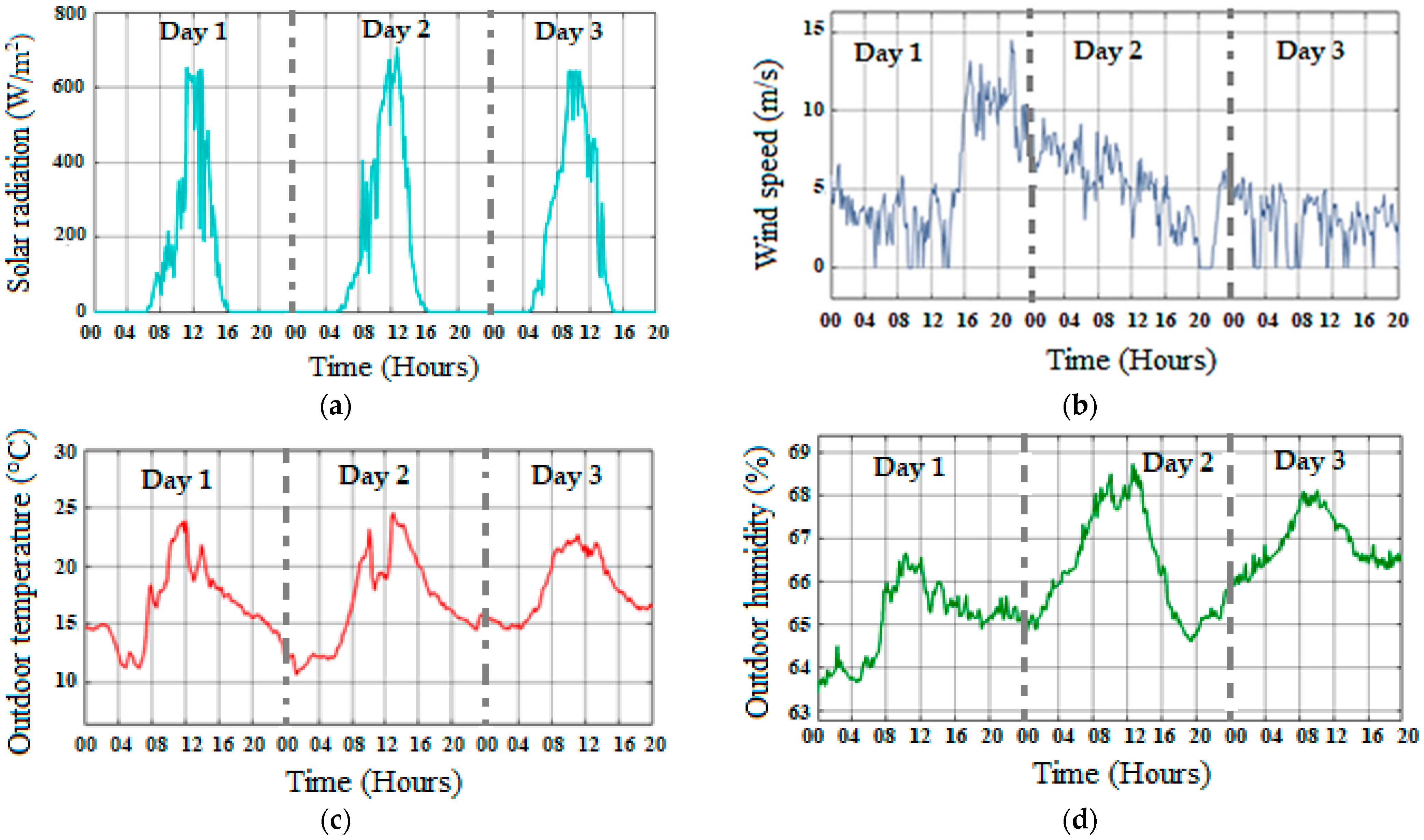
• HMP155A sensors to monitor the indoor and outdoor temperatures of the greenhouse, in order to ensure that the desired conditions are maintained. The accuracy of the temperature is ±0.4 °C and the operating range is contained between −24 °C and 48 °C. For the humidity, the accuracy is ±3% in the range of 0 to 100%.
• Anemometers are used to measure wind speed, which is essential for understanding air circulation and its impact on temperature and humidity.
• The Kipp & Zonen pyranometer (manufactured by OTT Hydromet company, France) is used to measure solar radiation with an accuracy of ±5%.
• Thermocouples are used to measure the temperature of the cover and the sandwich panel of the SIG.
• The IR120 sensor is a temperature sensor designed for measuring the canopy temperature.
• PT-107 sensors are used to measure the soil temperature inside the greenhouse.

Figure 4 presents the different sensors in the SIG.

3.3. Thermal Modeling of SIG

3.3.1. Heat Balance

The thermal balance describing the dynamic evolution of the indoor air temperature of the greenhouse T_in is computed by using the following equation [43]:

$$\frac{\mathrm{d}{\mathrm{T}}_{\mathrm{i}\mathrm{n}}}{\mathrm{d}\mathrm{t}}=\frac{1}{{\mathrm{d}}_{\mathrm{a}}{\mathrm{C}}_{\mathrm{a}}\mathrm{V}}\left({\mathrm{Q}}^{\mathrm{S}\mathrm{o}\mathrm{l}\mathrm{a}\mathrm{r},\mathrm{r}\mathrm{a}\mathrm{d}\mathrm{i}\mathrm{a}\mathrm{t}\mathrm{i}\mathrm{o}\mathrm{n}}+{\mathrm{Q}}^{\mathrm{H}\mathrm{T} \mathrm{c}\mathrm{a}\mathrm{n}\mathrm{o}\mathrm{p}\mathrm{y}}+{\mathrm{Q}}^{\mathrm{H}\mathrm{T} \mathrm{c}\mathrm{o}\mathrm{v}\mathrm{e}\mathrm{r}}+{\mathrm{Q}}^{\mathrm{H}\mathrm{T} \mathrm{g}\mathrm{r}\mathrm{o}\mathrm{u}\mathrm{n}\mathrm{d}}-{\mathrm{Q}}^{\mathrm{I}\mathrm{n}\mathrm{f}\mathrm{i}\mathrm{l}\mathrm{t}\mathrm{r}\mathrm{a}\mathrm{t}\mathrm{i}\mathrm{o}\mathrm{n}}\right)$$

(1)

with d_a denoting the air density [1.25 Kg·m⁻³], C_a denoting the air heat capacity [1003 J·Kg⁻¹·°C⁻¹], and V denoting the greenhouse volume.

The increase in thermal energy resulting from the transmission of solar radiation through the covering [48] is as follows:

$${\mathrm{Q}}^{\mathrm{S}\mathrm{o}\mathrm{l}\mathrm{a}\mathrm{r},\mathrm{r}\mathrm{a}\mathrm{d}\mathrm{i}\mathrm{a}\mathrm{t}\mathrm{i}\mathrm{o}\mathrm{n}}={\mathrm{Q}}^{\mathrm{S}\mathrm{R}\mathrm{I}}{\mathsf{\rho }}_{\mathrm{t}}(1-\mathsf{\alpha })$$

(2)

where Q^SRI is the entire solar radiation (comprising direct, diffuse, and reflected components) that falls upon the outer surface of the cover, ${\mathsf{\rho }}_{\mathrm{t}}$ represents the transmissivity of the greenhouse cover, and α takes into account the latent heat flux-to-net radiation ratio.

The heat transfers due to the interaction between the canopy and the indoor air (Watt or Joules per second) is as follows:

$${\mathrm{Q}}^{\mathrm{H}\mathrm{T} \mathrm{C}\mathrm{a}\mathrm{n}\mathrm{o}\mathrm{p}\mathrm{y}}=\frac{\mathrm{K}\ast \mathrm{A}({\mathrm{T}}_{\mathrm{i}\mathrm{n}}-{\mathrm{T}}_{\mathrm{o}\mathrm{u}\mathrm{t}})}{\mathrm{d}}$$

(3)

where K is the thermal conductivity of the material (W/m. K), A is the surface area of the material through which the heat is conducted (m²) and d is its thickness in meters.

The heat transfer interaction between the cover and the indoor air can be calculated with the following equation:

$${\mathrm{Q}}^{\mathrm{H}\mathrm{T} \mathrm{c}\mathrm{o}\mathrm{v}\mathrm{e}\mathrm{r}}={\mathrm{U}}_{\mathrm{C}}\ast {\mathrm{S}}_{\mathrm{g}}({\mathrm{T}}_{\mathrm{i}\mathrm{n}}-{\mathrm{T}}_{\mathrm{o}\mathrm{u}\mathrm{t}})$$

(4)

where U_C is the overall heat transfer coefficient of the cover structure and S_g is the surface of the greenhouse.

The heat exchange between the soil and the indoor climate is as follows:

$${\mathrm{Q}}^{\mathrm{H}\mathrm{T} \mathrm{g}\mathrm{r}\mathrm{o}\mathrm{u}\mathrm{n}\mathrm{d}}={\mathrm{U}}_{\mathrm{g}}\ast {\mathrm{S}}_{\mathrm{g}}({\mathrm{T}}_{\mathrm{i}\mathrm{n}}-{\mathrm{T}}_{\mathrm{g}\mathrm{r}\mathrm{o}\mathrm{u}\mathrm{n}\mathrm{d}})$$

(5)

where Ug is the overall heat transfer coefficient of the ground structure (W/m²·°C), and Sg is the surface area of the SIG.

The heat reduction due to infiltration is as follows:

$${\mathrm{Q}}^{\mathrm{I}\mathrm{n}\mathrm{f}\mathrm{i}\mathrm{l}\mathrm{t}\mathrm{r}\mathrm{a}\mathrm{t}\mathrm{i}\mathrm{o}\mathrm{n}}={\mathrm{d}}_{\mathrm{a}}\ast {\mathrm{C}}_{\mathrm{a}}\ast \mathrm{R}\mathrm{E}({\mathrm{T}}_{\mathrm{i}\mathrm{n}}-{\mathrm{T}}_{\mathrm{o}\mathrm{u}\mathrm{t}})$$

(6)

where C_a is the air density (kg/m³), d_a is the specific heat of the air (J/kg·°C), and RE is the infiltration or air exchange rate (air changes per unit of time).

3.3.2. Thermal Balance

The dynamic model of the indoor relative humidity in the greenhouse can be determined by using [49]:

$$\frac{\mathrm{d}{\mathrm{H}}_{\mathrm{i}\mathrm{n}}}{\mathrm{d}\mathrm{t}}=\frac{1}{{\mathrm{d}}_{\mathrm{a}}\mathrm{V}}{(\mathrm{Q}}^{\mathrm{e}\mathrm{v}\mathrm{a}\mathrm{p}}-{\mathrm{V}}^{\mathrm{C}\mathrm{o}\mathrm{o}\mathrm{l}\mathrm{i}\mathrm{n}\mathrm{g}}({\mathrm{H}}_{\mathrm{i}\mathrm{n}}-{\mathrm{H}}_{\mathrm{o}\mathrm{u}\mathrm{t}}))$$

(7)

where H_in and H_out represent the indoor and outdoor relative humidity values, V^Cooling is the ventilation rate, and Q^evap is the evapotranspiration rate resulting from the soil evaporation and crop transpiration, which can be calculated as follows:

$${\mathrm{Q}}^{\mathrm{e}\mathrm{v}\mathrm{a}\mathrm{p}}={\mathrm{V}\mathrm{C}}_{\mathrm{e}}{\mathrm{s}}_{\mathrm{w}\mathrm{i}\mathrm{n}\mathrm{d}}({\mathrm{P}}_{\mathrm{o}\mathrm{u}\mathrm{t}}-{\mathrm{P}}_{\mathrm{i}\mathrm{n}})$$

(8)

where s_wind is the wind speed, P_out and P_in are, respectively, the outdoor and indoor saturated vapor pressure values, Ce denotes the transfer coefficient of water vapor in the air, and V is the greenhouse volume.

3.3.3. Indoor Climate under Control

In the context of controlling the air conditions within the greenhouse and activating various actuators (such as the heating system or cooling system), Equation (1) is updated to reflect the specific control actions and relationships between the variables in this controlled environment, by adding the heat exchanges due to the cooling and heating:

$$\frac{\mathrm{d}{\mathrm{T}}_{\mathrm{i}\mathrm{n}}}{\mathrm{d}\mathrm{t}}=\frac{1}{{\mathrm{d}}_{\mathrm{a}}{\mathrm{C}}_{\mathrm{a}}\mathrm{V}}\left({\mathrm{Q}}^{\mathrm{s}\mathrm{o}\mathrm{l}\mathrm{a}\mathrm{r} \mathrm{r}\mathrm{a}\mathrm{d}\mathrm{i}\mathrm{a}\mathrm{t}\mathrm{i}\mathrm{o}\mathrm{n}}+{\mathrm{Q}}^{\mathrm{H}\mathrm{T} \mathrm{c}\mathrm{a}\mathrm{n}\mathrm{o}\mathrm{p}\mathrm{y}}+{\mathrm{Q}}^{\mathrm{H}\mathrm{T} \mathrm{c}\mathrm{o}\mathrm{v}\mathrm{e}\mathrm{r}}+{\mathrm{Q}}^{\mathrm{H}\mathrm{T} \mathrm{g}\mathrm{r}\mathrm{o}\mathrm{u}\mathrm{n}\mathrm{d}}-{\mathrm{Q}}^{\mathrm{I}\mathrm{n}\mathrm{f}\mathrm{i}\mathrm{l}\mathrm{t}\mathrm{r}\mathrm{a}\mathrm{t}\mathrm{i}\mathrm{o}\mathrm{n}}{-\mathrm{Q}}^{\mathrm{C}\mathrm{o}\mathrm{o}\mathrm{l}\mathrm{i}\mathrm{n}\mathrm{g}}+{\mathrm{Q}}^{\mathrm{h}\mathrm{e}\mathrm{a}\mathrm{t}\mathrm{i}\mathrm{n}\mathrm{g}}\right)$$

(9)

where Q^Cooling (Wm⁻²) is the rate of heat lost from the greenhouse by activating the ventilation system, which can be calculated as follows:

$${\mathrm{Q}}^{\mathrm{C}\mathrm{o}\mathrm{o}\mathrm{l}\mathrm{i}\mathrm{n}\mathrm{g}}={\mathrm{V}}^{\mathrm{C}\mathrm{o}\mathrm{o}\mathrm{l}\mathrm{i}\mathrm{n}\mathrm{g}}{\mathrm{C}}_{\mathrm{a}}{\mathrm{d}}_{\mathrm{a}}({\mathrm{T}}_{\mathrm{o}\mathrm{u}\mathrm{t}}-{\mathrm{T}}_{\mathrm{i}\mathrm{n}})$$

(10)

Q^Heating (Wm⁻²) is the heat provided by the heating system; it is defined as follows [35]:

$${\mathrm{Q}}^{\mathrm{H}\mathrm{e}\mathrm{a}\mathrm{t}\mathrm{i}\mathrm{n}\mathrm{g}}=\frac{{\mathrm{N}}_{\mathrm{h}}{\mathrm{R}}_{\mathrm{h}}}{{\mathrm{S}}_{\mathrm{s}}}$$

(11)

where N_h denotes the number of heaters, S_s denotes the surface of the greenhouse, and R_h denotes the capacity of the heating system.

When the actuators are activated, it is necessary to include the humidifying and dehumidifying supplied by the humidification system in Equation (7). Consequently, the updated model for the relative humidity is defined by the following equation:

$$\frac{\mathrm{d}{\mathrm{H}}_{\mathrm{i}\mathrm{n}}}{\mathrm{d}\mathrm{t}}=\frac{1}{{\mathrm{d}}_{\mathrm{a}}\mathrm{V}}{(\mathrm{Q}}^{\mathrm{e}\mathrm{v}\mathrm{a}\mathrm{p}}-{\mathrm{V}}^{\mathrm{C}\mathrm{o}\mathrm{o}\mathrm{l}\mathrm{i}\mathrm{n}\mathrm{g}}\ast ({\mathrm{H}}_{\mathrm{i}\mathrm{n}}-{\mathrm{H}}_{\mathrm{o}\mathrm{u}\mathrm{t}}))+{\mathrm{Q}}_{\mathrm{H}\mathrm{u}\mathrm{m}\mathrm{i}\mathrm{d}}-{\mathrm{Q}}_{\mathrm{D}\mathrm{e}\mathrm{h}\mathrm{u}\mathrm{m}\mathrm{i}\mathrm{d}}$$

(12)

In particular, Q_Humid is the humidity rate supplied by the humidifying system and Q_Dehumid is the rate at which humidity is removed by the dehumidifying system.

4. Control Strategy and Contributions

The design of an FLC starts with the initial phase of specifying the input and output parameters as well as linguistic variables. To move from numerical data to linguistic variables (fuzzy values) [14], the fuzzification process is employed. In the subsequent phase, fuzzy rules that encompass membership functions are utilized to articulate human expertise, which is essentially a logical connection between the input and output parameters. The defuzzification is executed, involving the calculation of a numerical outcome based on the fuzzy rules. The FLC methodology consists of three main steps that should be applied sequentially as shown in Figure 5.

The FLC represents a robust methodology within the realm of artificial intelligence. It offers the capability to address control challenges encountered in nonlinear and multivariable systems, as exemplified by its application within a greenhouse setting. The outdoor temperature and humidity are the primary climatic factors affecting the indoor air conditions of the greenhouse. In this research, two FLC models that are fine-tuned to safeguard the indoor temperature and humidity levels are proposed:

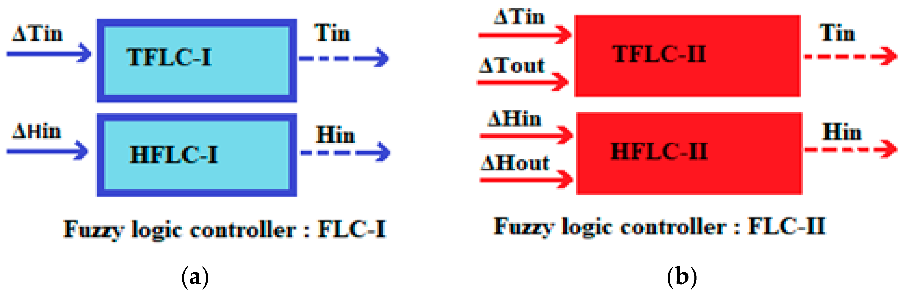
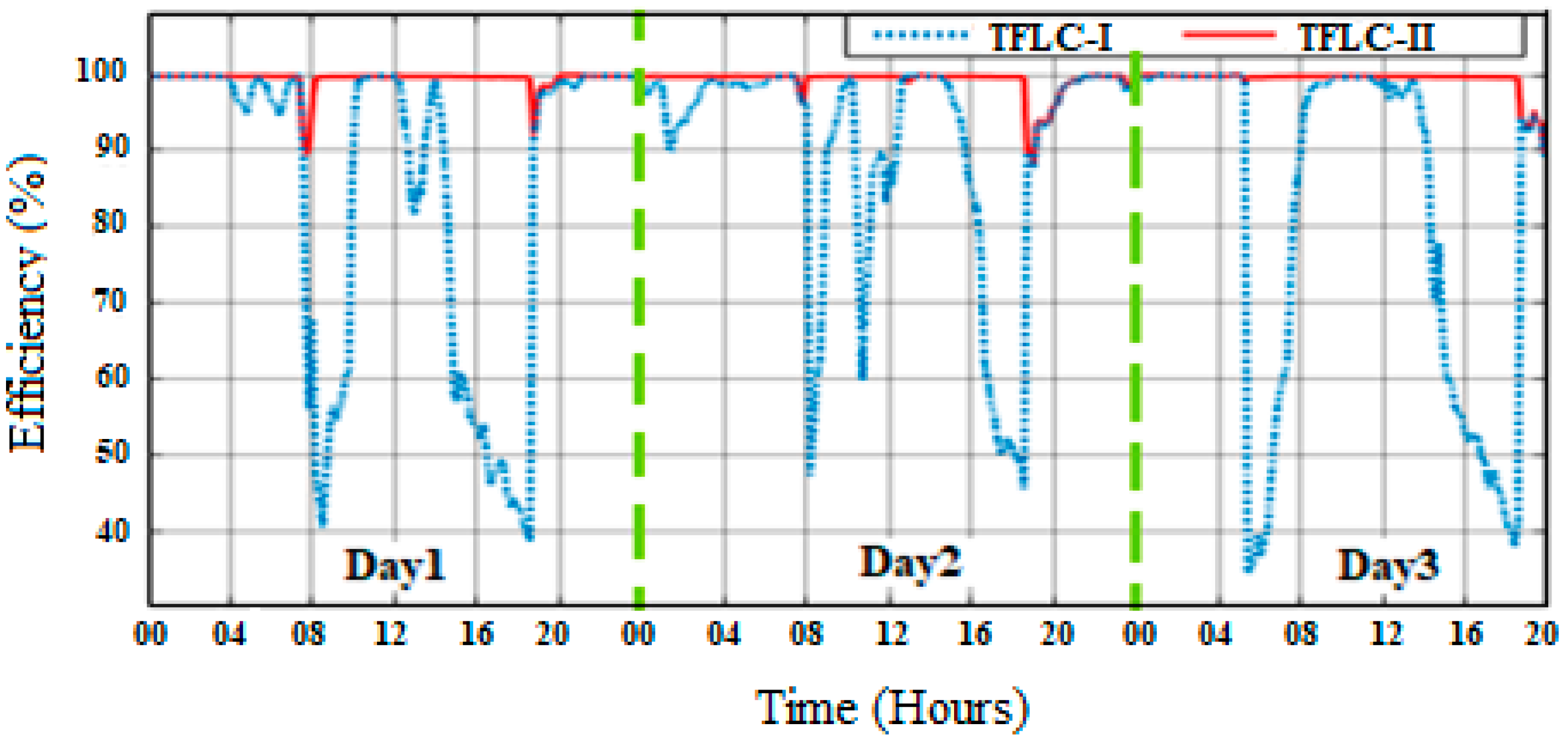
• The first FLC model, named FLC-I, employs the error of the indoor temperature (ΔT_in) as the input state variable for controlling the indoor temperature (TFLC-I) and the error of indoor humidity (ΔH_in) as the input state variable for controlling the indoor humidity (HFLC-I).
• The second FLC model, named FLC-II, is based on two input variables for controlling the temperature and two input variables for controlling the humidity. The input variables for controlling the indoor temperature (TFLC-II) are the error of the indoor temperature (ΔT_in) and the error of the outdoor temperature (ΔT_out). Instead, the input variables for controlling the indoor relative humidity (HFLC-II) are the error of indoor humidity (ΔH_in) and the error of outdoor humidity (ΔH_out).

Figure 6 presents the two different fuzzy logic models (FLC-I Figure 6a and FLC-II Figure 6b).

The indoor climate control system is based on FLCs that manage the decisions required to obtain an optimum climate in the greenhouse, based on the meteorological data and user instructions. These decisions are applied to the indoor greenhouse by electrical equipment (cooling system, heating system, humidifier, and dehumidifier system). This approach exhibits strong robustness and adaptability.

In the design of a fuzzy logic controller (FLC), selecting the criteria involves defining linguistic variables, terms, and rules that govern the system’s behavior. For the proposed greenhouse control system, this entails defining the input variables of the fuzzy logic control, followed by selecting the linguistic terms for each input with a range defining their variation. Membership functions describe the degree to which input values belong to each linguistic term, while the output variables represent the control actions or decisions made by the FLC. These are defined by linguistic terms specific to the actuators installed in the greenhouse. In the final stage, the fuzzy rules determine how input variables relate to output variables. The following section presents the details of the various fuzzy logic controllers developed.

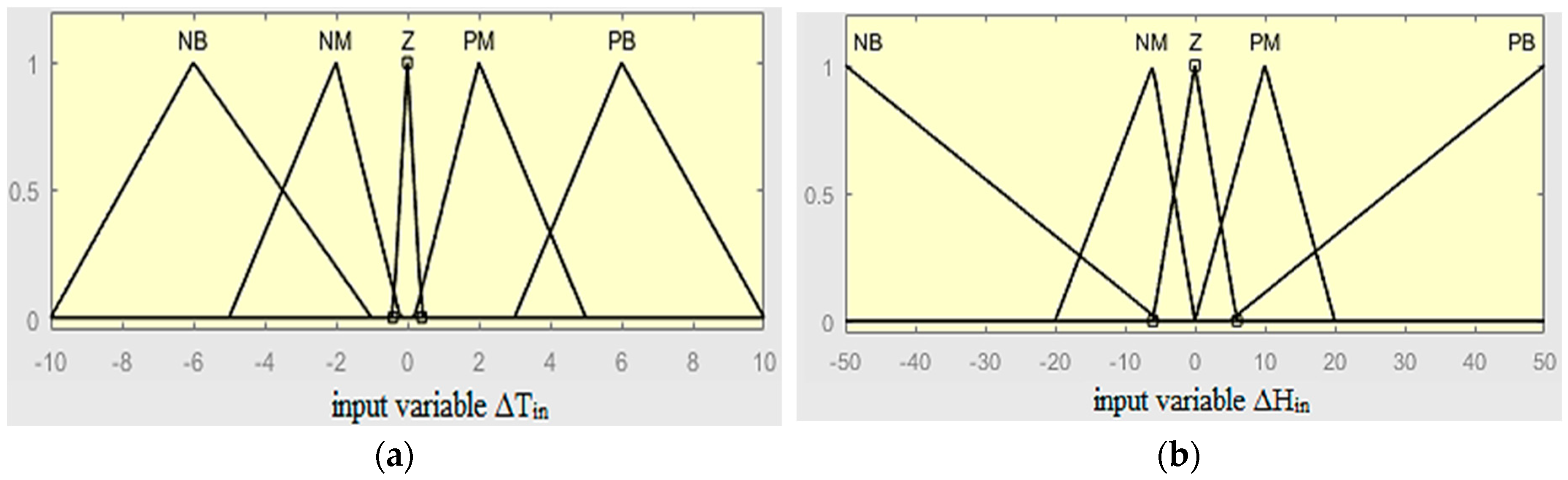
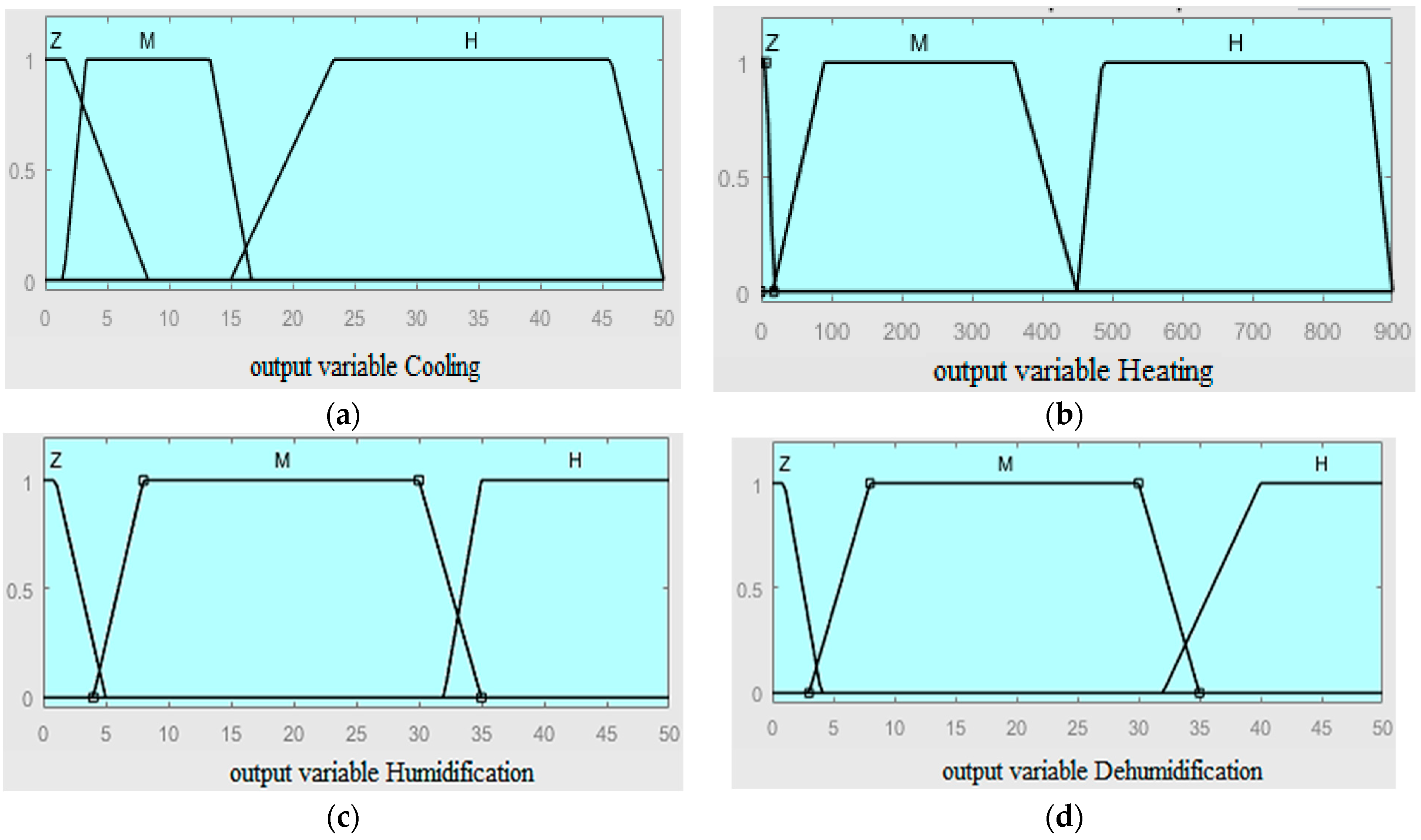
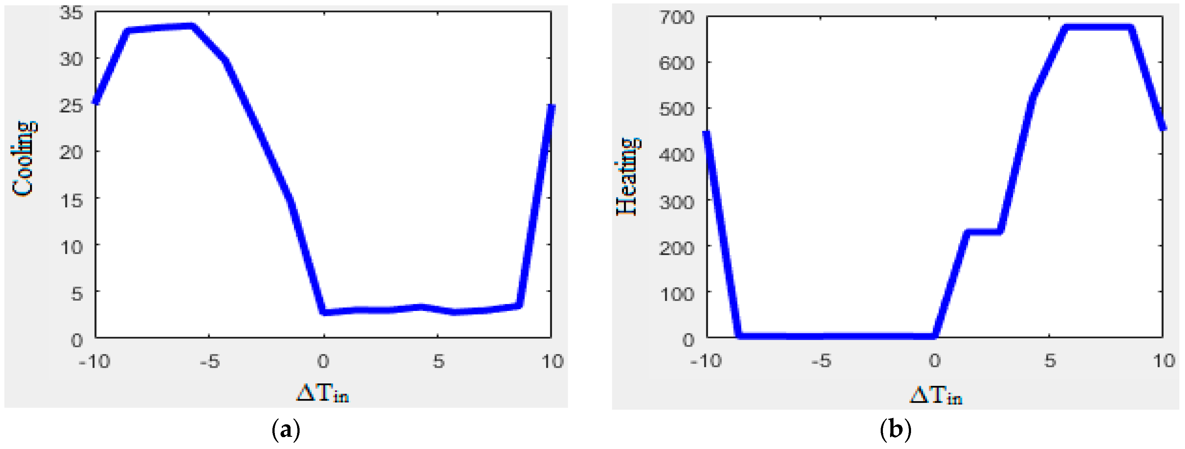
4.1. Fuzzy Logic Controller I (FLC-I)

The FLC-I (Figure 6a) is composed of two input variables and two output control variables. The input variables to control the indoor temperature and indoor relative humidity are defined on five fuzzy sets {Negative Big «NB», Negative Medium «NM», Zero «Z», Positive Medium «PM», Positive Big «PB»}, whereas the control variables are defined with three fuzzy sets {Zero «Z», Medium «M», High «H»}.

After numerous simulation tests of the FLC-I, the ranges of fuzzy sets for the input variables ΔT_in and ΔH_in were selected as follows:

For ΔT_in: NB (Negative Big): [−10 to −1], NM (Negative Medium): [−5 to −0.2], Z (Zero): [−0.4 to 0.4], PM (Positive Medium): [0.2 to 5], PB (Positive Big): [3 to 10].

The indoor temperature (T_in) and humidity (H_in) are compared with prefixed optimal values, known as T_opt and H_opt, respectively, restituting ΔT_in, ΔH_in (Figure 7), where we have the following:

ΔT_in = T_opt − T_in

(13)

ΔH_in = H_opt − H_in

(14)

Figure 7 shows the membership functions of the input variable of FLC-I: Figure 7a presents the fuzzification input of the indoor temperature control and Figure 7b reports the fuzzification input of the indoor relative humidity control.

The output fuzzy variables related to the status of these actuators (cooling (CO), heating (HE), humidification (HU), and dehumidification system (DH)) are categorized as zero, medium, or high, where “zero” signifies that they are not activated, “medium” implies activation at the medium level, and “high” indicates activation at the maximum level.

Figure 8 describes the membership functions of the output variables for FLC-I. The output variables for the temperature control include the cooling rate and the heating rate (Figure 8a and Figure 8b, respectively). Additionally, the outputs for the fuzzy control of humidity, such as the humidification rate and dehumidification rate, are presented in Figure 8c and Figure 8d, respectively.

The fuzzy set ranges for the cooling and heating output variables are divided as follows:

The cooling system becomes active when the indoor temperature surpasses the optimal value. This activation is governed by the following fuzzy set ranges:

Z = [0 to 8], M = [1 to 16], H = [15 to 50].

When the indoor temperature falls below the optimal level, the heating system is triggered. This activation operates within the fuzzy set ranges:

Z = [0 to 18], M = [17 to 450], H = [450 to 900].

The humidification system becomes active when the indoor humidity falls below the optimal level. This activation is based on fuzzy set ranges, as follows:

Z = [0 to 5], M = [4 to 35], H = [32.5 to 50].

The dehumidification system is triggered to reduce indoor humidity toward the optimal value. This activation occurs within fuzzy set ranges, as follows:

Z = [0 to 4], M = [3 to 35], H = [32.5 to 50].

The inference rules for FLC-I are presented in

Table 3. Fuzzy rules of temperature control.

ΔTin	Cooling (CO)	Heating (HE)
NB	High	Zero
NM	Medium	Zero
Z	Zero	Zero
PM	Zero	Medium
PB	Zero	High

and

Table 4. Fuzzy rules of humidity control.

ΔHin	Humidification (HU)	Dehumidification (DH)
NB	Zero	High
NM	Zero	Medium
Z	Zero	Zero
PM	Medium	Zero
PB	High	Zero

, based on the Mamdani rules composition.

Dedicated inference rules for indoor temperature control are as follows:

• IF (ΔT_in) is (NB, NM, Z, PM, PB) THEN (CO) is (zero, medium, and high) and (HE) is (zero, medium, high).
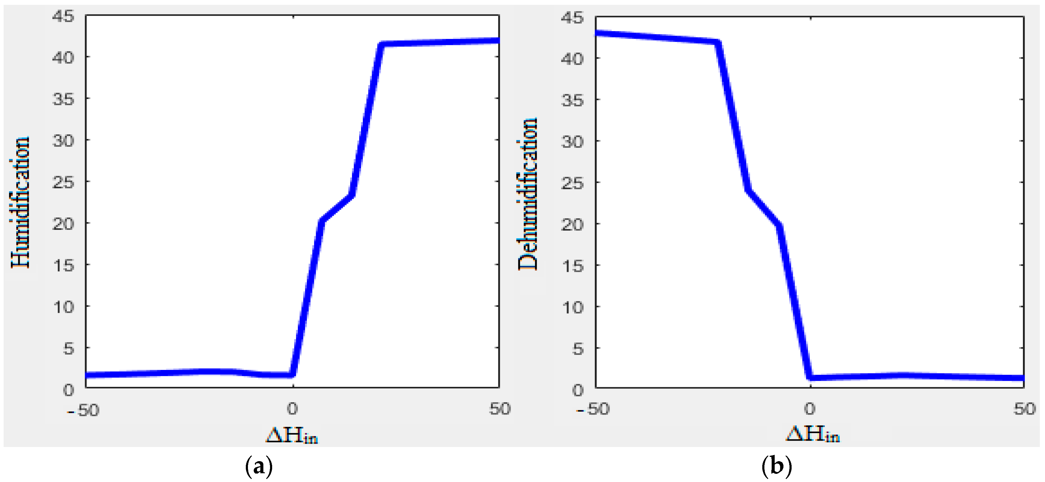
• Dedicated inference rules for indoor humidity control are as follows:
• IF (ΔH_in) is (NB, NM, Z, PM, PB) THEN (HU) is (zero, medium, and high) and (DU) is (zero, medium, and high).

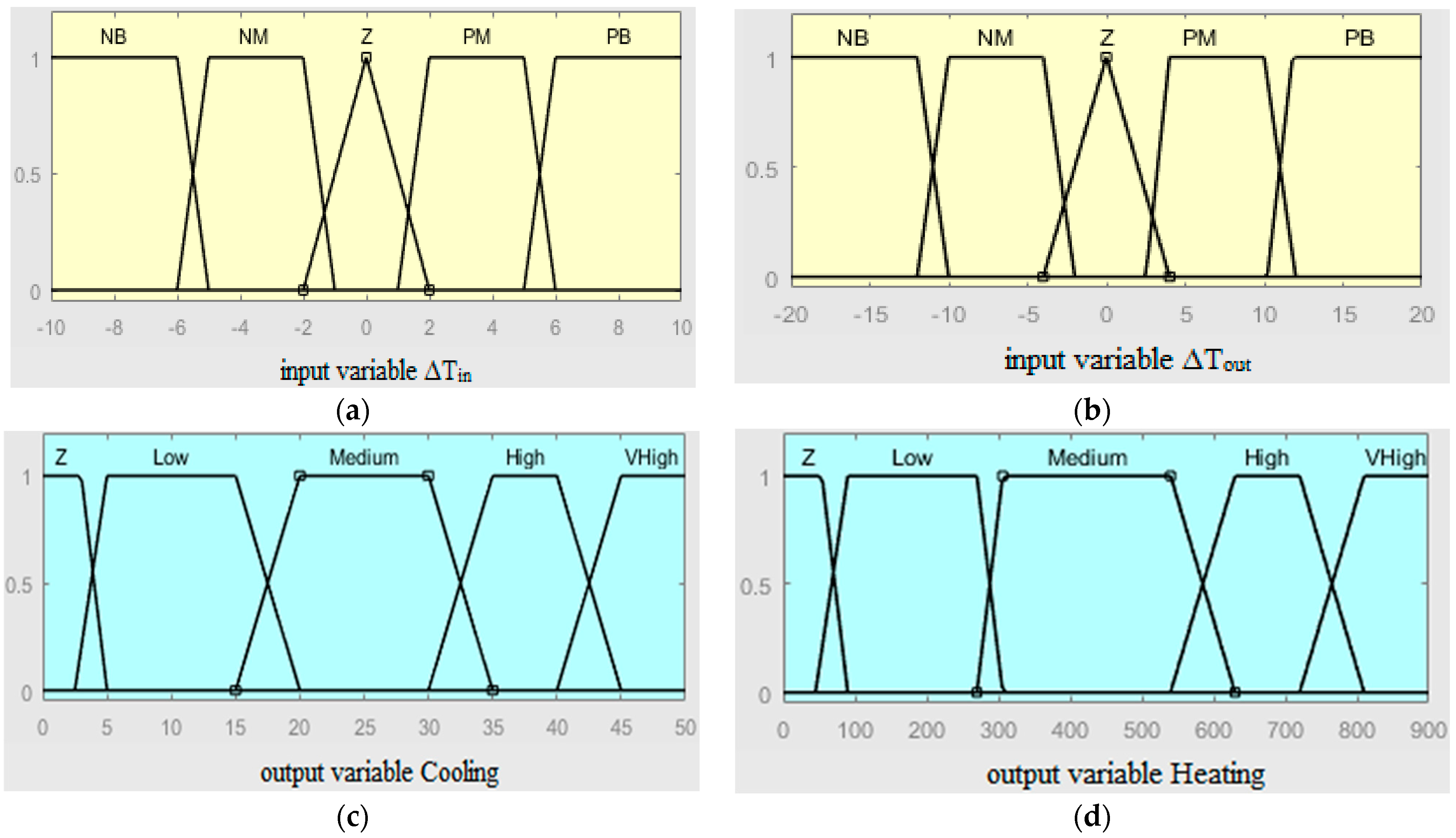
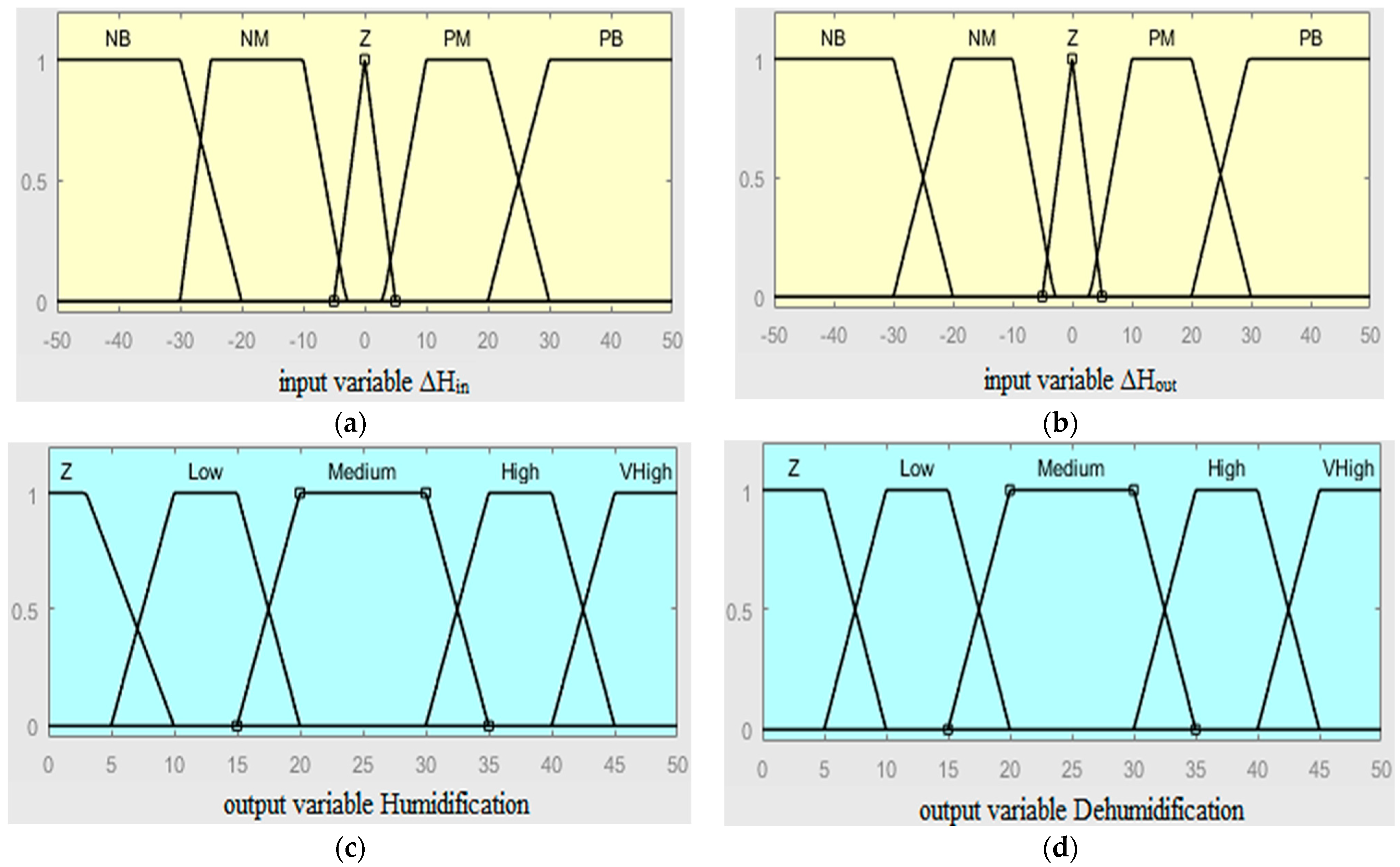
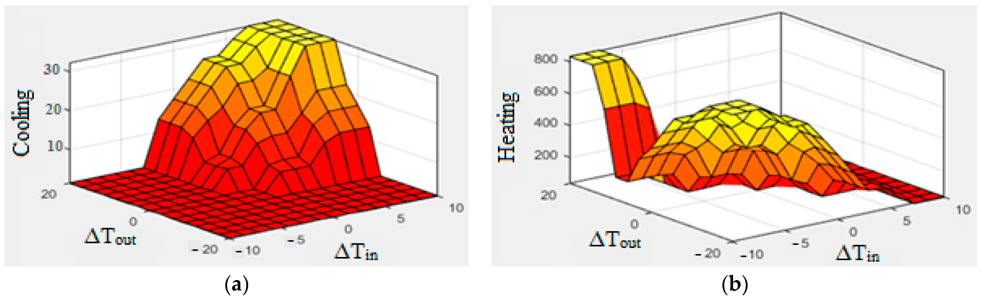
4.2. Fuzzy Logic Controller II (FLC-II)

The model of FLC-II is developed to control the indoor temperature and humidity, based on two input variables for each controlled climatic parameter. The two inputs are defined on five fuzzy sets {Negative Big «NB», Negative Medium «NM», Zero «Z», Positive Medium «PM», Positive Big «PB»}, and the output variables are defined by five fuzzy sets {Zero «Z», Low «L», Medium «M», High «H», Very High «VH»}.

4.2.1. Temperature Fuzzy Logic II (TFLC-II)

TFLC-II (Figure 6b) is based on two input variables: ΔT_in, defined in Equation (13), and ΔT_out defined as follows:

ΔT_out = T_opt − T_out

(15)

i.e., the difference between the optimal value, T_opt, and the outdoor temperature.

The output variables are the cooling and heating rates. The membership functions of the input and output variables of TFLC-II are reported in Figure 9.

The ranges of fuzzy sets of inputs variable ΔT_in and ΔH_out are defined as follows:

ΔT_in = NB: [−10 to −5]; NM: [−6 to −1]; Z: [−2 to 2]; PM: [1 to 6]; PB: [5 to 10].

ΔT_out = NB: [−20 to −10]; NM: [−12 to −2]; Z: [−4 to 4]; PM: [2.5 to 12]; PB: [10 to 20].

The ranges of fuzzy sets for the output variables of the cooling and heating systems were selected as follows:

Cooling rate = Z: [0 to 5]; Low: [2.5 to 20]; Medium: [15 to 35]; High: [30 to 45]; VHigh: [40 to 50], and heating rate = Z: [0 to 90]; Low: [50 to 305]; Medium: [260 to 618]; High: [543 to 810]; VHigh: [720 to 900].

The inference rules, applied to control the indoor temperature under TFLC-II, are presented in

Table 5. Inference rules for TFLC-II.

ΔTin ΔTout	NB	NM	Z	PM	PB
NB	HE(VHigh)	HE(High)	HE(Medium)	HE(Low)	HE(Z)
NM	HE(High)	HE(Medium)	HE(Low)	HE(Z)	C(Z)
Z	HE(Medium)	HE(Low)	HE(Z)	C(Low)	C(Medium)
PM	HE(Low)	HE(Z)	C(Low)	C(Medium)	C(High)
PB	HE(Z)	C(Z)	C(Medium)	C(VHigh)	C(VHigh)

and based on the Mamdani rules composition:

If (ΔT_in) is (NB, NM, Z, PM, PB) and (ΔT_out) is (NB, NM, Z, PM, PB), then cooling (C) is (Z, L, M, H, VH) and heating (HE) is (Z, L, M, H, VH).

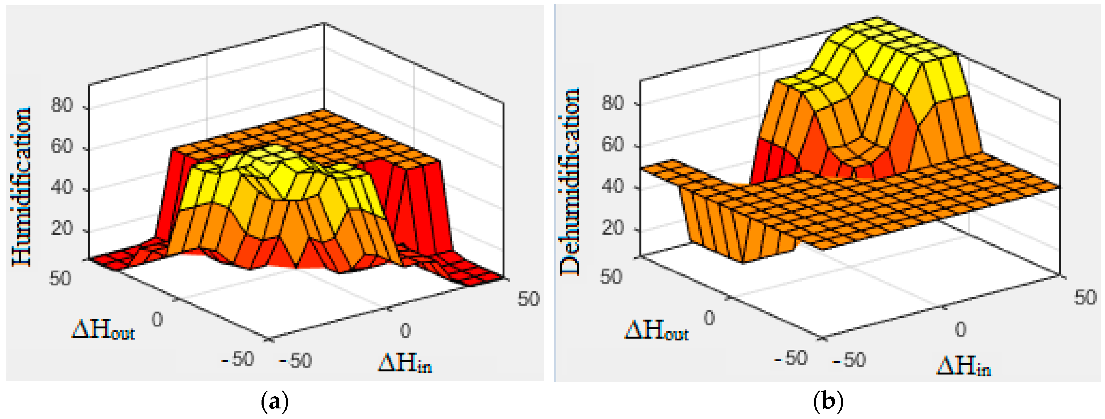
4.2.2. Humidity Fuzzy Logic II (HFLC-II)

HFLC-II (Figure 6b) is based on two input variables: ΔH_in, defined in Equation (14), and ΔH_out, defined as follows:

ΔH_out = H_opt − H_out

(16)

i.e., the difference between the optimal value, H_opt, and the outdoor humidity. The output variables of the fuzzy logic are the humidification and the dehumidification rates.

The membership functions of the input and output variables are presented in Figure 10. The ranges of fuzzy sets of inputs variable ΔT_in and ΔH_out were selected as follows: ΔH_in and ΔH_out = NB: [−50 to −20]; NM: [−30 to −4]; Z: [−5 to 5]; PM: [4 to 30]; PB: [20 to 50].

The output variation of the humidification and dehumidification system is defined with five fuzzy sets ranges, as follows: humidification and dehumidification rate = Z: [0 to 10]; Low: [5 to 20]; Medium: [15 to 35]; High: [30 to 45]; VHigh: [40 to 50].

The inference rules, applied to control the indoor humidity under HFLC-II, are presented in

Table 6. Inference rules for HFLC-II.

ΔHin ΔHout	NB	NM	Z	PM	PB
NB	H(VHigh)	H(High)	H(Medium)	H(Low)	H(Z)
NM	H(High)	H(Medium)	H(Low)	H(Z)	DH(Z)
Z	H(Medium)	H(Low)	H(Z)	DH(Low)	DH(Medium)
PM	H(Low)	H(Z)	DH(Low)	DH(Medium)	DH(High)
PB	H(Z)	DH(Medium)	DH(High)	DH(VHigh)	DH(VHigh)

and based on the Mamdani rules composition:

If (ΔH_in)) is (NB, NM, Z, PM, PB) and (ΔH_out) is (NB, NM, Z, PM, PB), then humidification (H) is (Z, L, M, H, VH) and dehumidification (DH) is (Z, L, M, H, VH).

5. Results and Discussion

5.1. Definition of Time Series Data

The implementation of the experimental approach on the described SIG is based on time series measurements for three specific days: 13, 14, and 15 April 2021, from 00:00 on the first day to 20:00 on the third day.

The outdoor and indoor climatic conditions have a direct impact on the microclimate inside the SIG. The time-domain outdoor variables are the solar radiation (Figure 11a), the wind speed (Figure 11b), the outdoor temperature (Figure 11c), and the humidity (Figure 11d). The solar radiation reaches 700 W/m² with a temperature varying between 11.2 °C and 24.8 °C; the relative humidity varies from 63.8% to 68.8% and the wind speed reaches a maximum value of 14.9 m/s.

The temperature of the canopy refers to the air temperature within the upper portion of the greenhouse, typically near the top of the plants. The canopy temperature is critical because it affects the temperature at which the leaves and upper parts of the plants are exposed, and this can influence the transpiration rates and the overall health of the plants. Then, the ground temperature influences the root development, the nutrient uptake, and the microbial activity in the soil. Cooler soil can slow down the root growth and nutrient absorption.

Figure 12 reports the different temperatures, due to different heat exchanges in the greenhouse: the canopy temperature (green curve) is calculated by Equation (3), the cover temperature (blue curve) is calculated by Equation (4), and the ground temperature (brown curve) in the greenhouse is calculated by Equation (5).

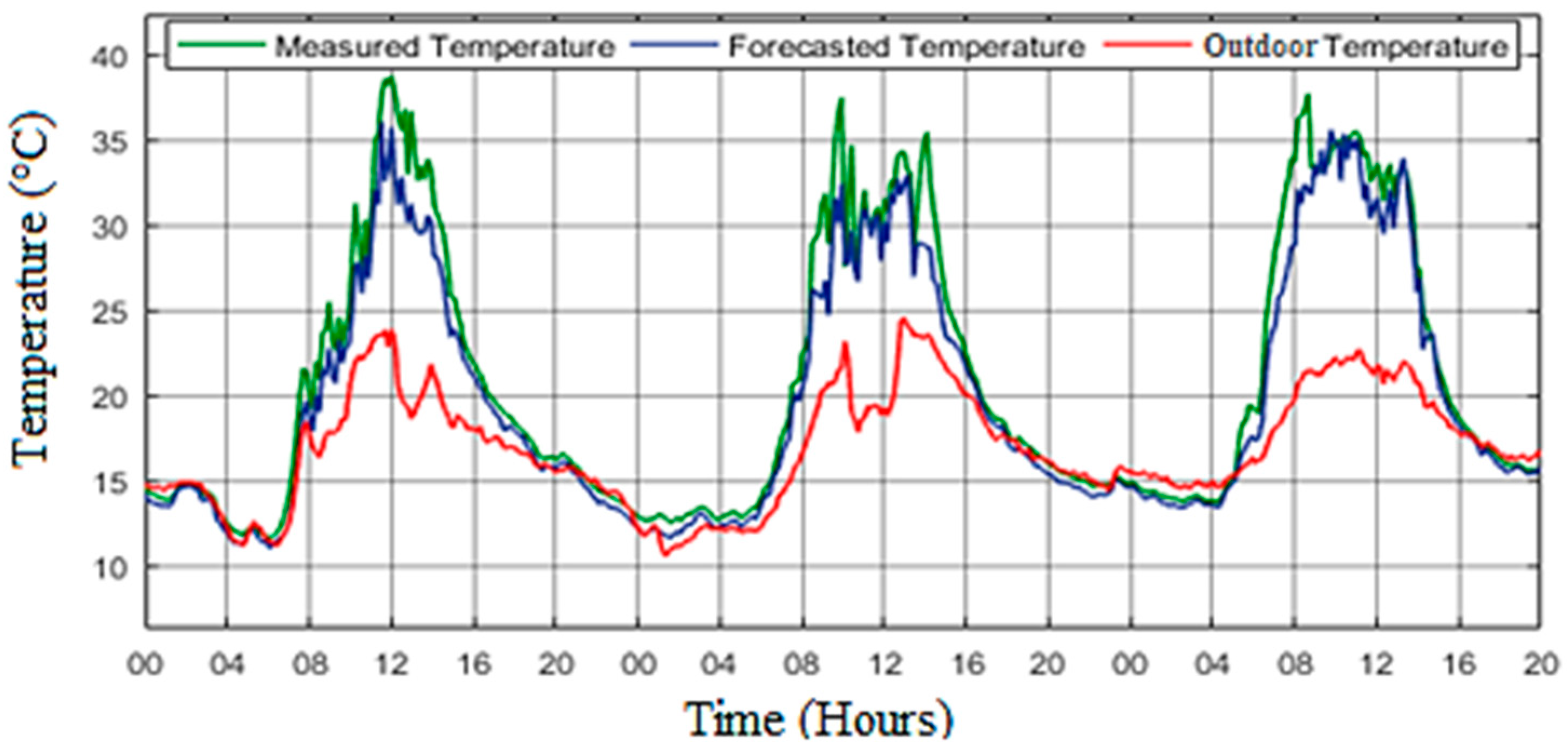
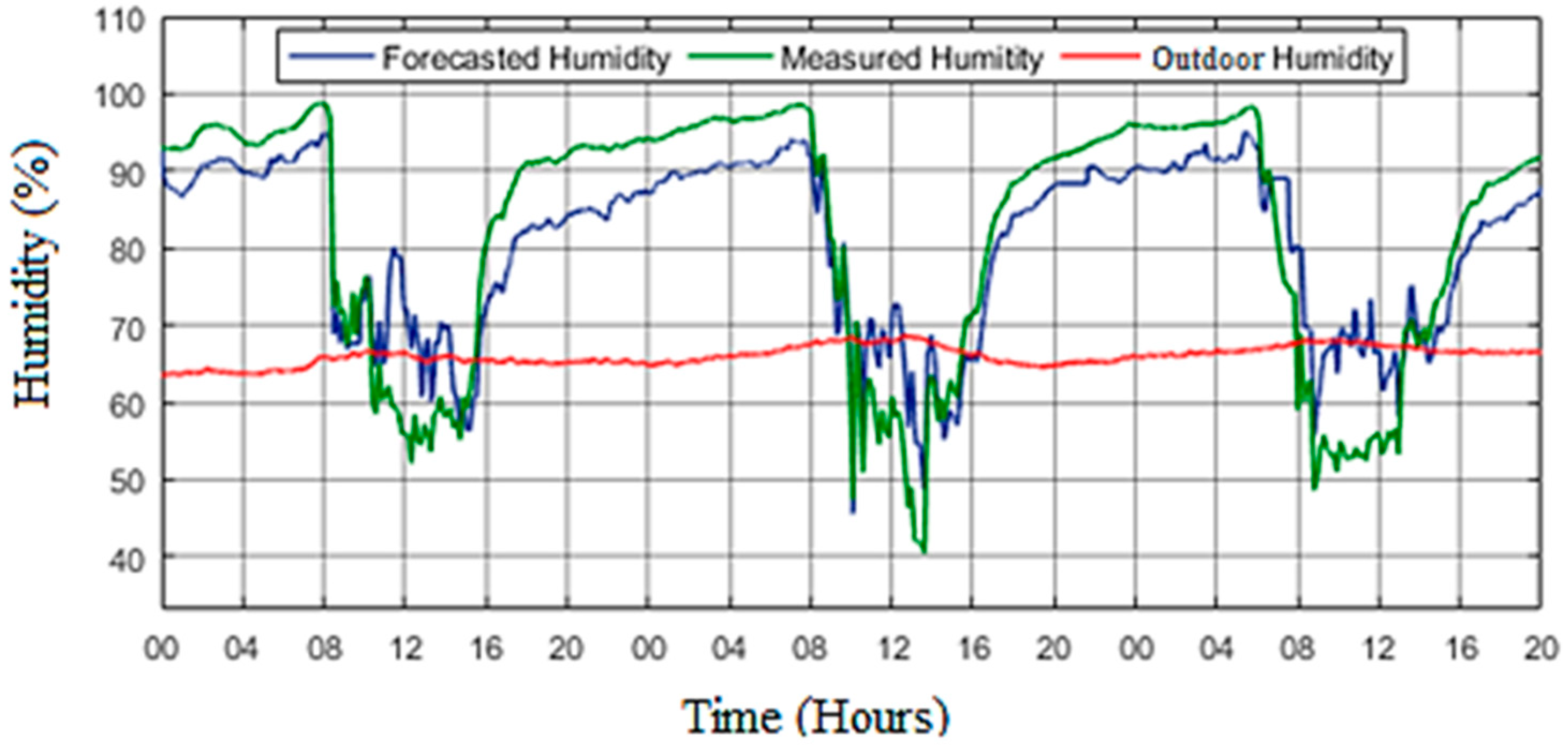
5.2. Experimental Validation and Performance Model

A physical model of the insulated greenhouse was implemented in the MATLAB/Simulink environment. To assess the accuracy of this model, a comparison was carried out between the theoretical model outputs and actual experimental measurements. This comparison helps to validate the model’s predictive capabilities and its ability to accurately simulate the indoor climate of the greenhouse.

The forecasted temperature and humidity are the factors predicted by the greenhouse model. The calculation of the forecasted temperature and humidity is based on a mathematical model of the greenhouse with various inputs, such as weather data, greenhouse design parameters, and control strategies. Finally, they are calculated using Equations (1) and (7), respectively.

The purpose of calculating the forecasted temperature and humidity is to validate the experimental greenhouse model and enhance the effectiveness of the model by comparison with the experimental process. A small difference between the measured and forecasted factors (RMSE) suggests that the model accurately predicts temperature and humidity variations and responds effectively to environmental changes. On the other hand, the forecasted temperature and humidity are essential for greenhouse management as they help growers make informed decisions about ventilation, heating, cooling, and irrigation strategies to maintain optimal growing conditions for their crops.

Figure 13 displays the time series of the air temperatures in the greenhouse. It includes the measured temperature (green curve), the forecasted temperature (blue curve), which iscalculated using Equation (1), and the outdoor temperature (red curve).

Figure 14 presents the time-series relative humidity. The measured humidity is represented by the green curve, the forecasted humidity, calculated by Equation (7), is shown by the blue curve, and the red curve reports the outdoor humidity.

Figure 13 and Figure 14 reveal a notable agreement between the forecasted and measured values of the indoor temperature and relative humidity. To evaluate the efficacy of the dynamic model, the statistical estimators RMSE, TSSE, MAPE, and EF have been calculated. These estimators are employed to scrutinize and assess the model performance. They provide quantitative measures to gauge the accuracy and reliability of the model predictions in comparison to the actual data. The simulation results are presented in

Table 7. Statistical analysis of the parameters indoor the smart greenhouse.

Climatic Variables	RMSE	TSSE	MAPE (%)	EF (%)
Air temperature	0.017 °C	1.36 °C	0.022	98.29
Relative humidity	0.071%	1.29%	0.026	90.98

.

The statistical analysis proves that the efficiency of the implemented dynamic model to predict the time series of the temperature and the relative humidity inside the SIG. In fact, the values of RMSE are equal to 0.017 °C for the temperature and 0.071 for the relative humidity. The MAPE returns a value equal to 0.022% for the temperature and 0.026% for the relative humidity. Moreover, the EF is the efficacy of the model to calculate the indoor variables of the greenhouse and the value 98.29% for the temperature shows a high linear correlation between the forecasted and measured variables, while EF is equal to 90.98% for the relative humidity.

5.3. Effects and Performance of Different FLC Strategies

To compare the performance of the different FLCs, two optimal temperatures are fixed: 25 °C during the daytime and 15 °C at night. Additionally, the optimal humidity is applied with 70% humidity during the test time, considering the specific needs of the plant growth. FLC-I and FLC-II are implemented, in order to show the performance of the best controller to regulate the indoor climate of a greenhouse system.

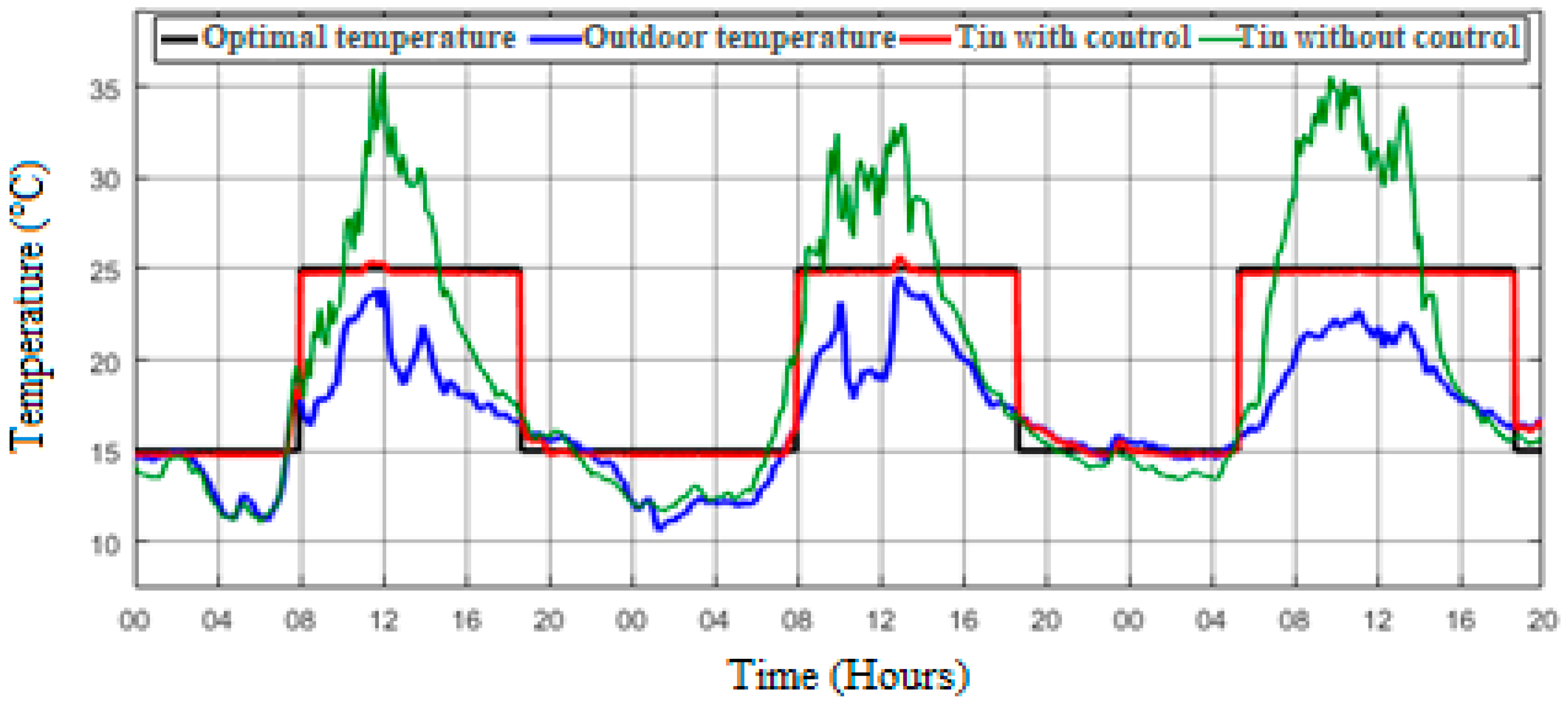
5.3.1. Indoor Temperature Control

The outcomes of the indoor temperature (T_in) by applying TFLC-I and TFLC-II, respectively, are depicted in Figure 15 and Figure 16.

In the first hours of the first two days, from 00:00 to 08:00, the uncontrolled indoor temperature (green curve) drops to a low of 4 °C. On the other hand, the temperature under TFLC-I (red curve in Figure 15) fluctuates around the optimal temperature (black curve) with variations in some hours. Furthermore, the indoor temperature under TFLC-II (Figure 16) consistently aligns with the optimal temperature, which is due to the implementation of the outdoor temperature (blue curve) as a critical factor for regulating the indoor temperature. During the night, a heating rate is applied in the greenhouse to increase the indoor temperature to around the optimal temperature, 15 °C. Conversely, during the day, the indoor temperature without control can increase up to 36 °C, deviating by 11 °C from the optimal temperature of 25 °C. In this case, the cooling system is activated to extract the hot air. It is worth noting that the indoor temperature under TFLC-I decreases to approach the optimal temperature with a similar disturbance. During the same period, the TFLC-II is employed to regulate the indoor temperature, and it successfully reduces it to the optimal values, demonstrating a strong agreement between the controlled and the desired temperature.

In Figure 17 and Figure 18, you can observe the cooling rate generated by the ventilation systems and the heating flow rate through the heating pump. These mechanisms are employed to attain and maintain the desired air temperature within the greenhouse. The control of these systems under TFLC-I is determined by the error of indoor temperature. Instead, the error of both indoor and outdoor temperatures determines the control of the actuators under TFLC-II. As already explained, these errors represent the variation between the optimal temperature and the actual indoor and outdoor temperatures.

The cooling flow rate increases when 8 °C ≤ ΔT_in ≤ 10 °C due to the change in the optimal temperature range from 15 °C to 25 °C (observed at 08:00, as shown in Figure 16). Consequently, in this scenario, the heating system decreases from 700 to 500.

Similarly, the heating system decreases when −10 °C ≤ ΔT_in ≤ −8 °C. This occurs because, during certain periods of the daytime, the heating system becomes active to raise the indoor temperature toward the optimal value of 25 °C (for instance, at 10:00 on the first day). As the indoor temperature exceeds the optimal value, the heating system decreases toward zero.

In Figure 18, the results of the cooling and heating system using FLC-II demonstrate a strong agreement between the fuzzy rules and the variations in the cooling and heating rates during the fluctuations in the indoor temperature.

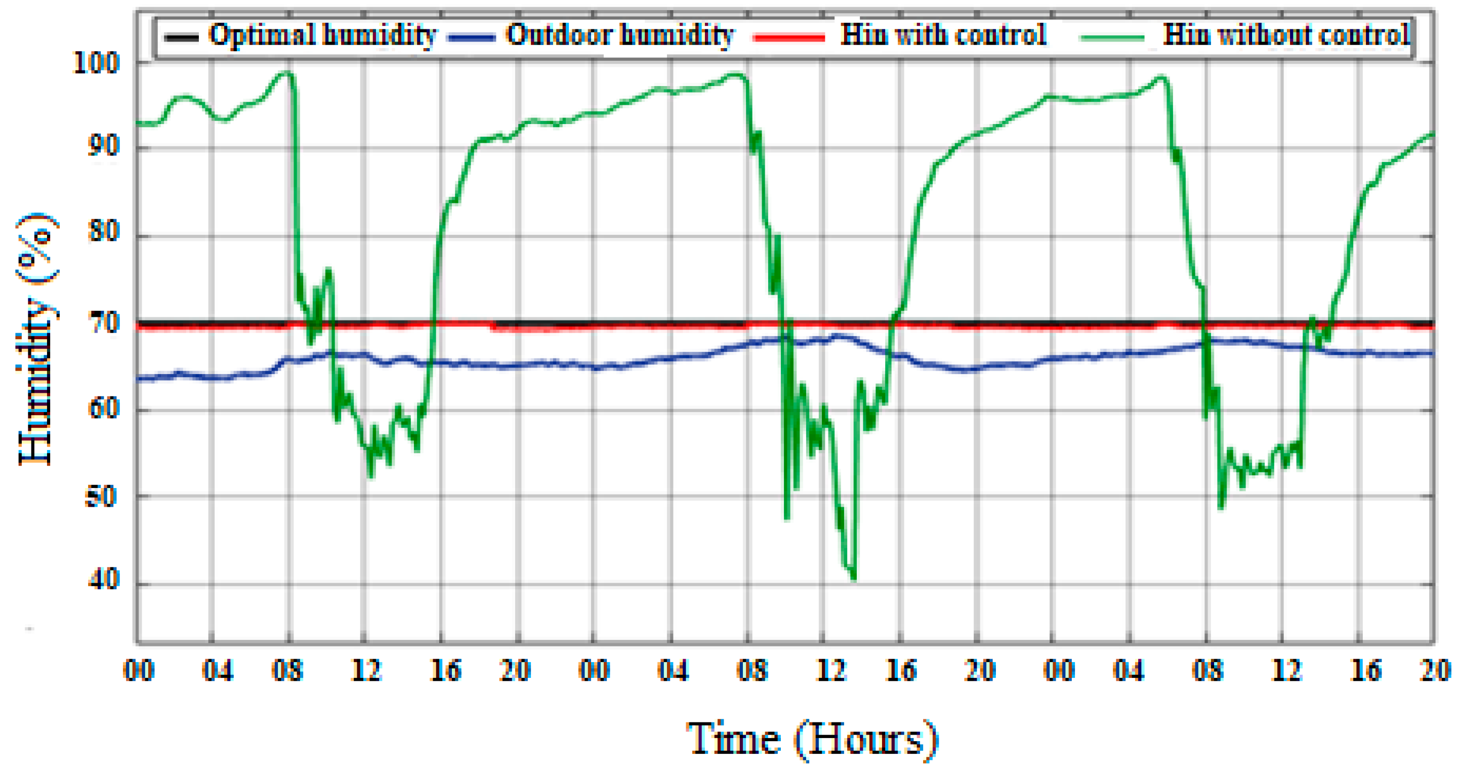
5.3.2. Indoor Humidity Control

The simulation results for the relative humidity in the SIG, both with and without control, are depicted in Figure 19 (for HFLC-I) and Figure 20 (for HFLC-II). These figures illustrate how HFLC-I and HFLC-II affect the regulation of the indoor relative humidity (H_in) within the SIG, providing valuable insights into the effectiveness of these control systems in maintaining the desired humidity levels.

During the nighttime hours, the relative humidity inside the greenhouse, if uncontrolled, remains at a high level of 98% (green curve). This humidity level experiences variations corresponding to the fluctuations in the outdoor humidity, which typically range between 64% and 69% (blue curve). The recommended or optimal humidity for cultivating tomatoes in this greenhouse is around 70% (black curve).

In the experiments, the results from the two different FLCs (HFLC-I and HFLC-II) demonstrate a substantial agreement between the controlled humidity (red curve) and the optimal humidity. However, it is worth noting that HFLC-II exhibits a higher level of precision in regulating the indoor relative humidity (the indoor humidity equal to 70%) compared to HFLC-I (the indoor humidity equal to 68%). Then, this discrepancy is especially noticeable between the hours of 19:00 and 08:00.

Figure 21 and Figure 22 illustrate the changes in the rates of humidification and dehumidification carried out by the actuators. In these figures, HFLC-I bases its decisions on the error of indoor humidity, while HFLC-II takes into account both indoor and outdoor humidity errors. Furthermore, during the nighttime, the dehumidification rate reaches a value of 43 gH₂O/min, aimed at reducing the indoor humidity within the greenhouse. Conversely, during the daytime, the humidification system is activated at a rate of 42 gH₂O/min to maintain the humidity levels around the optimal value, which is 70%.

5.3.3. Performance of the FLCs

The performance evaluation of the FLC system is a vital strategy to assess its effectiveness in managing the greenhouse environment. This evaluation involves the use of various metrics to gauge the performance of the control units. A comparison between the two FLC models, FLC-I and FLC-II, is conducted for both air temperature and relative humidity. The results of this comparative analysis are presented in

Table 8. Performance of FLCs to regulate the indoor climate.

Fuzzy Logic Controllers		RMSE (%)	MAPE (%)	EF (%)
FLC-I	Temperature	1.87	6.04	85.40
	Humidity	0.24	0.61	99.34
FLC-II	Temperature	0.69	1.84	99.35
	Humidity	0.23	0.17	99.86

. This table provides a comprehensive overview of how the two FLC systems perform in regulating the air temperature and relative humidity, allowing for a thorough assessment of their respective strengths and weaknesses.

FLC-I demonstrates its performance through an RMSE of 1.87% for temperature and 0.24% for humidity. Additionally, it exhibits substantial efficiency, with an EF of 85.40% for temperature and 99.34% for humidity. The values of MAPE are equal to 6.04% and 0.61%, respectively. Comparatively, FLC-II outperforms fuzzy logic FLC-I, showcasing a smaller RMSE of 0.69% for temperature and 0.23% for relative humidity. This superior accuracy is reflected in high control efficacy, with efficiency values EF reaching 99.35% for temperature and 99.86% for humidity. The results show the enhanced performance of FLC-II in accurately controlling the indoor variables of the greenhouse.

The effectiveness of the FLC-II stems from the incorporation of the outdoor temperature and outdoor humidity into the control strategy of the FLC. These outdoor factors play a crucial role as inputs in the rules of inference, allowing the controller to make more informed and context-aware decisions.

By considering outdoor temperature and humidity, FLC-II enhances its control strategy also considering the dynamic conditions outside the SIG. This integration enables the controller to respond more effectively to outdoor influences, resulting in improved accuracy and efficiency in regulating the indoor environment. The contribution of outdoor variables enriches the decision-making process, making FLC-II a robust and adaptive control system for the smart greenhouse.

In Figure 23, the time-domain performances of FLC-I and FLC-II during the temperature control are addressed. TFLC-I exhibits efficacy fluctuations between 40% and 99.9%. Notably, its performance decreases to 40% during the day (07:00 to 20:00) and rises to the range of 90% to 99.9% during the night (20:00 to 07:00). This instability in FLC-I during the day is significantly influenced by the outdoor temperature (not calculated in the inferences rules). On the other hand, TFLC-II demonstrates more stable performance, varying between 90% and 90.9% during the night, achieving precision and stability at 99.98%. Despite slight variations during changes in outdoor temperature at 08h and 19h, FLC-II maintains stability and reaches a commendable efficiency of 99.9%.

The performance fluctuations observed in HFLC-I and HFLC-II for controlling relative humidity mirror the variations resulting from the stability of the outdoor humidity; anyway, which consistently remains around 99% (Table 8).

Table 9. Comparative analysis indexes between the different literature methods and the proposed method in this paper with respect to temperature (T) and humidity (H).

Methods	RMSE (T)	EF (T)	RMSE (H)	EF (H)
Proposed model prediction	0.017	98.29	0.071	90.98
Proposed FLC-II control efficacy	0.69	99.35	0.23	99.86
Accuracy of the greenhouse model [47]	1.94	--	3.16	--
Predict the dynamic model of the greenhouse [49]	0.17	57.8	0.07	99.8
Neural network predicting model [4]	0.271	--	0.481	--
Predicting model based on intelligence artificial [50]	0.82	--	--	--
Data-driven robust model predictive control for temperature control [51]	0.32 (0.60)	--	--	--
Threshold control [52]	1.19	--	1.14	--
Model predictive control For one second [52]	0.28	--	0.15	--
PI controller [53]	1.59	--	--	--
Model predictive control (MPC) [54]	3.01 2.45	--	--	--

reports a comparison between the method proposed in this paper and the methods present in the literature to predict the greenhouse model and efficacy of FLC to regulate indoor climatic variables.

The strengths of this research can be succinctly outlined as follows (Table 9): in Tunisia, a greenhouse system was devised [47] to validate the climate conditions and enhance the energy efficiency within the agricultural greenhouses. The RMSE values obtained for the temperature and the relative humidity were 1.94 °C and 3.16%, respectively. Subsequently, in [49], a dynamic model for predicting air temperature and relative humidity was experimentally validated, and the values of RMSE and EF were equal to 0.17 °C and 57.8%, respectively, for the indoor temperature, and 0.07 °C and 99.8% for the indoor relative humidity. Ref. [4] constructed a neural network model for greenhouse microclimate predictions and the statistical assessments indicated RMSE values of 0.271 °C and 0.481% for temperature and humidity, respectively. Ref. [50] achieved a dynamic model for the indoor temperature based on artificial intelligence, reporting RMSE equal to 0.82 °C. Ref. [51] focuses on data-driven robust model predictive control for the greenhouse temperature control and energy utilization assessment, obtaining an RMSE value equal to 0.32 for the first day and 0.60 for the second day. Instead, the EF of the proposed model without control of the indoor temperature and relative humidity reaches 98.29% and 90.98%, respectively (Table 7). Furthermore, EF of FLC-II achieved impressive results, registering 99.35% and 99.86% for indoor temperature and relative humidity, respectively (Table 8). The proposed fuzzy logic controller in this study is compared with other control methods, as presented in Table 9. Ref. [52] examines Threshold control, yielding RMSE values of 1.19 for temperature and 1.14 for humidity. PWM control, as reported by the same reference, achieves values of 0.28 for temperature and 0.15 for humidity for one hour. Ref. [53] introduces a PID controller for temperature control, resulting in an RMSE of 1.59. Ref. [54] focuses on model predictive control (MPC) for regulating the temperature of two greenhouse systems, with RMSE values of 3.01 and 2.45, respectively.

Based on these results, the algorithm of FLC-II is more adaptable than that of FLC-I to control the indoor climatic variables of the greenhouse. Therefore, it explains the importance of outdoor climatic variables to regulate the indoor climate of an agricultural greenhouse. These high percentages underscore the control system’s effectiveness in enhancing the accuracy and precision of the model. The findings reveal greater accuracy, as evidenced by a comparably low RMSE and a higher EF value for both controlled and uncontrolled scenarios, setting it apart from existing scientific research in the literature.

The accuracy of fuzzy logic control in the greenhouse model suggests a promising avenue for designing and testing new technologies to tackle specific challenges in greenhouse management. These challenges encompass reducing energy consumption, enhancing crop yield, and mitigating environmental impact. Additionally, the forecasting of internal climatic conditions within the greenhouse, coupled with an intelligent fuzzy logic controller, offers a solution to automate the greenhouse system using IoT (Internet of Things) technologies and analytics to develop predictive models with machine learning for crop growth. These results also provide a comprehensive study on the application of novel control technologies, such as irrigation systems, and the integration of renewable energy sources for powering various electronic devices within the greenhouse.

6. Conclusions

This work contributes to defining an efficient and effective strategy to maintain a favorable indoor climate of an SIG based on experimental validation, which is supported by data monitoring sensors. Physical modeling based on different studies of the heat exchanges in the greenhouse is developed in order to attain an optimal microclimate for the plants. The statistical analysis demonstrates a robust agreement between forecasted and measured variables for the greenhouse model, as indicated by small RMSE and high EF. Specifically, for the temperature, the RMSE is 0.017 °C with an EF of 98.29%, and, for humidity, the RMSE is 0.071% with an EF equal to 90.98% (Table 7).

According to the control of the indoor climatic parameters of the SIG, FLC-I and FLC-II are implemented to compare their performance. The results carried out for the temperature control reveal that FLC-II performs better than FLC-I, achieving an EF equal to 99.35% compared to 85.40%, respectively. The efficacy of FLCs for the relative humidity control demonstrates high efficacy, with FLC-II exhibiting an EF of 99.86% compared to the EF of FLC-I equal to 99.34% (Table 8).

Furthermore, the study delves into the performance of the control strategy during cold and hot periods. The findings suggest that FLC is more stable and reliable during the night compared to the daytime for the indoor temperature and relative humidity.

References

1. Katzin, D.; Van-Henten, J.; Van-Mourik, S. Process-based greenhouse climate models: Genealogy, current status, and future directions. Agric. Syst. 2022, 198, 103388. [Google Scholar] [CrossRef]
2. Guo, Y.; Zhao, H.; Zhang, S. Modeling and optimization of environment in agricultural greenhouses for improving cleaner and sustainable crop production. J. Clean. Prod. 2021, 285, 124843. [Google Scholar] [CrossRef]
3. Belhaj, S.L.; Fourati, F. A greenhouse modeling and control using deep neural networks. Appl. Artif. Intell. 2021, 35, 1905–1929. [Google Scholar] [CrossRef]
4. Petrakis, T.; Kavga, A.; Thomopoulos, V. Neural Network Model for Greenhouse Microclimate Predictions. Agriculture 2022, 12, 780. [Google Scholar] [CrossRef]
5. Costantino, A.; Comba, L.; Sicardi, G. Energy performance and climate control in mechanically ventilated greenhouses: A dynamic modelling-based assessment and investigation. Appl. Energy 2021, 288, 116583. [Google Scholar] [CrossRef]
6. Hamad, I.H.; Chouchaine, A.; Bouzaouache, H. On modeling greenhouse air-temperature: An experimental validation. In Proceedings of the 2021 18th International Multi-Conference on Systems, Signals & Devices (SSD), Monastir, Tunisia, 22–25 March 2021; pp. 353–358. [Google Scholar]
7. Altes-Buch, Q.; Quoilin, S.; Lemort, V. A modeling framework for the integration of electrical and thermal energy systems in greenhouses. In Building Simulation; Tsinghua University Press: Beijing, China, 2022; pp. 1–19. [Google Scholar]
8. Howard, D.A.; Ma, Z.; Veje, C. Greenhouse industry 4.0—Digital twin technology for commercial greenhouses. Energy Inform. 2021, 4, 1–13. [Google Scholar] [CrossRef]
9. Ahmed, S.F.; Liu, G.; Mofijur, M. Physical and hybrid modelling techniques for earth-air heat exchangers in reducing building energy consumption: Performance, applications, progress, and challenges. Sol. Energy 2021, 216, 274–294. [Google Scholar] [CrossRef]
10. Torrente, C.J.; Reca, J.; López-Luque, R. Simulation model to analyze the spatial distribution of solar radiation in agrivoltaic Mediterranean greenhouses and its effect on crop water needs. Appl. Energy 2024, 353, 122050. [Google Scholar] [CrossRef]
11. Nauta, A.; Han, J.; Tasnim, S.H. A new greenhouse energy model for predicting the year-round interior microclimate of a commercial greenhouse in Ontario, Canada. Inf. Process. Agric. 2023; in press. [Google Scholar]
12. Adesanya, M.A.; Na, W.H.; Rabiu, A. TRNSYS simulation and experimental validation of internal temperature and heating demand in a glass greenhouse. Sustainability 2022, 14, 8283. [Google Scholar] [CrossRef]
13. Cai, W.; Wei, R.; Xu, L. A method for modelling greenhouse temperature using gradient boost decision tree. Inf. Process. Agric. 2022, 9, 343–354. [Google Scholar] [CrossRef]
14. Faniyi, B.; Luo, Z. A Physics-Based Modelling and Control of Greenhouse System Air Temperature Aided by IoT Technology. Energies 2023, 16, 2708. [Google Scholar] [CrossRef]
15. Jung, D.H.; Lee, T.S.; Kim, K.G. A deep learning model to predict evapotranspiration and relative humidity for moisture control in tomato greenhouses. Agronomy 2022, 12, 2169. [Google Scholar] [CrossRef]
16. Vanegas-Ayala, S.C.; Barón Velandia, J.; Leal Lara, D.D. A systematic review of greenhouse humidity prediction and control models using fuzzy inference systems. Adv. Hum. Comput. Interact. 2022, 2022, 8483003. [Google Scholar] [CrossRef]
17. Laktionov, I.; Vovna, O.; Kabanets, M. Computer-Oriented Method of Adaptive Monitoring and Control of Temperature and Humidity Mode of Greenhouse Production. Balt. J. Mod. Comput. 2023, 11, 202–225. [Google Scholar] [CrossRef]
18. Taki, M.; Ajabshirchi, Y.; Ranjbar, S.F. Modeling and experimental validation of heat transfer and energy consumption in an innovative greenhouse structure. Inf. Process. Agric. 2016, 3, 157–174. [Google Scholar] [CrossRef]
19. Mihalakakou, G.; Souliotis, M.; Papadaki, M. Applications of earth-to-air heat exchangers: A holistic review. Renew. Sustain. Energy Rev. 2022, 155, 111921. [Google Scholar] [CrossRef]
20. Fatnassi, H.; Bournet, P.E.; Boulard, T. Use of computational fluid dynamic tools to model the coupling of plant canopy activity and climate in greenhouses and closed plant growth systems: A review. Biosyst. Eng. 2023, 230, 388–408. [Google Scholar] [CrossRef]
21. Jeon, Y.; Cho, L.; Park, S. Canopy Temperature and Heat Flux Prediction by Leaf Area Index of Bell Pepper in a Greenhouse Environment: Experimental Verification and Application. Agronomy 2022, 12, 1807. [Google Scholar] [CrossRef]
22. Tahery, D.; Roshandel, R.; Avami, A. An integrated dynamic model for evaluating the influence of ground to air heat transfer system on heating, cooling and CO2 supply in Greenhouses: Considering crop transpiration. Renew. Energy 2021, 173, 42–56. [Google Scholar] [CrossRef]
23. Brækken, A.; Sannan, S.; Jerca, I.O. Assessment of heating and cooling demands of a glass greenhouse in Bucharest, Romania. Therm. Sci. Eng. Prog. 2023, 41, 101830. [Google Scholar] [CrossRef]
24. Hilal, Y.Y.; Khessro, M.K.; Van dam, J. Automatic water control system and environment sensors in a greenhouse. Water 2022, 14, 1166. [Google Scholar] [CrossRef]
25. Acciani, G.; Chiarantoni, E.; Fornarelli, G.; Vergura, S. A Feature Extraction Unsupervised Neural Network for Environmental Data Set. Neural Netw. 2003, 16, 427–436. [Google Scholar] [CrossRef] [PubMed]
26. Puliafito, V.; Vergura, S.; Carpentieri, M. Fourier, Wavelet and Hilbert-Huang Transforms for Studying Electrical Users in the Time and Frequency Domain. Energies 2017, 10, 188. [Google Scholar] [CrossRef]
27. García, E.; Soto-zarazúa, A.; Genaro, M.; Toledano-ayala, M. Applications of artificial neural networks in greenhouse technology and overview for smart agriculture development. Appl. Sci. 2020, 10, 3835. [Google Scholar] [CrossRef]
28. Zhou, X.; Liu, Q.; Katzin, D. Boosting the prediction accuracy of a process-based greenhouse climate-tomato production model by particle filtering and deep learning. Comput. Electron. Agric. 2023, 211, 107980. [Google Scholar] [CrossRef]
29. Belhaj salah, L.; Fourati, F. Deep Elman neural network for greenhouse modeling. In Proceedings of the 8th International Conference on Sciences of Electronics, Technologies of Information and Telecommunications (SETIT’18), Maghreb, Tunisia, 18–20 December 2018; Springer International Publishing: Berlin/Heidelberg, Germany, 2020; Volume 1, pp. 271–280. [Google Scholar]
30. López-cruz, I.L.; Fitz-rodríguez, E.; Torres-monsivais, J.C. Control strategies of greenhouse climate for vegetables production. In Biosystems Engineering: Biofactories for Food Production in the Century XXI; Springer: Berlin/Heidelberg, Germany, 2014; pp. 401–421. [Google Scholar]
31. Cristaldi, L.; Faifer, M.; Leone, G.; Vergura, S. Reference Strings for Statistical Monitoring of the Energy Performance of Photovoltaic Fields. In Proceedings of the IEEE-ICCEP 2015 International Conference on Clean Electrical Power, Taormina, Italy, 16–18 June 2015. [Google Scholar]
32. Tian, Y. Adaptive control and supply chain management of intelligent agricultural greenhouse by intelligent fuzzy auxiliary cognitive system. Expert Syst. 2022, 41, e13117. [Google Scholar] [CrossRef]
33. Chen, Q.; Hu, X. Design of intelligent control system for agricultural greenhouses based on adaptive improved genetic algorithm for multi-energy supply system. Energy Rep. 2022, 8, 12126–12138. [Google Scholar] [CrossRef]
34. Abbood, H.M.; Nouri, N.M.; Riahi, M. An intelligent monitoring model for greenhouse microclimate based on RBF Neural Network for optimal setpoint detection. J. Process Control 2023, 129, 103037. [Google Scholar] [CrossRef]
35. Morozova, M. Methodology for Controlling Greenhouse Microclimate Parameters and Yield Forecast Using Neural Network Technologies. In Advanced Information-Measuring Technologies and Systems I; Springer Nature: Cham, Switzerland, 2023; pp. 245–277. [Google Scholar]
36. Riahi, J.; Vergura, S.; Mezghani, D. Smart and renewable energy system to power a temperature-controlled greenhouse. Energies 2021, 14, 5499. [Google Scholar] [CrossRef]
37. Jiang, Z.; Yang, S.; Pang, Q. Biochar improved soil health and mitigated greenhouse gas emission from controlled irrigation paddy field: Insights into microbial diversity. J. Clean. Prod. 2021, 318, 128595. [Google Scholar] [CrossRef]
38. Riahi, J.; Vergura, S.; Mezghani, D. A combined PV-wind energy system for an energy saving greenhouse. In Proceedings of the 2020 IEEE International Conference on Environment and Electrical Engineering and 2020 IEEE Industrial and Commercial Power Systems Europe (EEEIC/I&CPS Europe), Madrid, Spain, 9–12 June 2020; pp. 1–6. [Google Scholar]
39. Chen, W.H.; Mattson, N.S.; You, F. Intelligent control and energy optimization in controlled environment agriculture via nonlinear model predictive control of semi-closed greenhouse. Appl. Energy 2022, 320, 119334. [Google Scholar] [CrossRef]
40. Haas, N.T.; Ierapetritou, M.; Singh, R. Advanced model predictive feedforward/feedback control of a tablet press. J. Pharm. Innov. 2017, 12, 110–123. [Google Scholar] [CrossRef]
41. Wang, Y.; Lu, Y.; Xiao, R. Application of nonlinear adaptive control in temperature of chinese solar greenhouses. Electronics 2021, 10, 1582. [Google Scholar] [CrossRef]
42. Ren, Y.; Wu, C.; Yoshinaga, T. A Fuzzy Logic Controller for Greenhouse Temperature Regulation System Based on Edge Computing. In International Conference on Mobile Networks and Management; Springer: Cham, Switzerland, 2021; pp. 316–332. [Google Scholar]
43. Riahi, J.; Vergura, S.; Mezghani, D. Intelligent control of the microclimate of an agricultural greenhouse powered by a supporting PV system. Appl. Sci. 2020, 10, 1350. [Google Scholar] [CrossRef]
44. Laktionov, I.; Vovna, O.; Kabanets, M. Information technology for comprehensive monitoring and control of the microclimate in industrial greenhouses based on fuzzy logic. J. Artif. Intell. Soft Comput. Res. 2023, 13, 19–35. [Google Scholar] [CrossRef]
45. Kurniawan, D.; Witanti, A. Prototype of control and monitor system with fuzzy logic method for smart greenhouse. Indones. J. Inf. Syst. 2021, 3, 116–127. [Google Scholar] [CrossRef]
46. Mostakim, N.; Mahmud, S.; Jewel, K.H. A simulation based study of A greenhouse system with intelligent fuzzy logic. Int. J. Fuzzy Log. Syst. 2020, 10, 19–37. [Google Scholar] [CrossRef]
47. Azaza, M.; Echaieb, K.; Enrico, F. An intelligent system for the climate control and energy savings in agricultural greenhouses. Energy Effic. 2016, 9, 1241–1255. [Google Scholar]
48. Efrén, F.R.; Chieri, K.; Gene, G.A.; Milton, E.T.; Sandra, W.B.; Margaret, M. Dynamic modeling and simulation of greenhouse environments under several scenarios: A web-based application. Comput. Electron. Agric. 2010, 70, 105–116. [Google Scholar]
49. Ali, R.B.; Bouadila, S.; Mami, A. Development of a Fuzzy Logic Controller applied to an agricultural greenhouse experimentally validated. Appl. Therm. Eng. 2018, 141, 798–810. [Google Scholar]
50. Hosseini, M.P.; Taki, M.; Abdanan Mehdizadeh, S. Prediction of Greenhouse Indoor Air Temperature Using Artificial Intelligence (AI) Combined with Sensitivity Analysis. Horticulturae 2023, 9, 853. [Google Scholar] [CrossRef]
51. Mahmood, F.; Govindan, R.; Bermak, A.; Yang, D.; Al-Ansari, T. Data-driven robust model predictive control for greenhouse temperature control and energy utilization assessment. Appl. Energy 2023, 343, 121190. [Google Scholar] [CrossRef]
52. Kazuhisa, I.; Tsubasa, T. Model predictive temperature and humidity control of greenhouse with ventilation. Procedia Comput. Sci. 2021, 192, 212–221. [Google Scholar]
53. Atia, D.M.; El-madany, H.T. Analysis and design of greenhouse temperature control using adaptive neuro-fuzzy inference system. J. Electr. Syst. Inf. Technol. 2017, 4, 34–48. [Google Scholar] [CrossRef]
54. Jung, D.; Kim, H.; Kim, J.Y. Model predictive control via output feedback neural network for improved multi-window greenhouse ventilation control. Sensors 2020, 20, 1756. [Google Scholar] [CrossRef]
Figure 1. Conceptual scheme of the SIG under test and its controls.
Smartcities 07 00055 g001
Figure 2. (a) Lateral view of the experimental SIG under test [3]; (b) dimensions of the greenhouse.
Smartcities 07 00055 g002aSmartcities 07 00055 g002b
Figure 3. CR5000 data acquisition unit.
Smartcities 07 00055 g003
Figure 4. Greenhouse equipment sensors: (a) HMP155A inside sensor; (b) IR120 canopy temperature sensor; (c) PT-107 sensor inside the greenhouse; (d) Kipp & Zonen pyranometer sensor.
Smartcities 07 00055 g004
Figure 5. Smart fuzzy logic design.
Smartcities 07 00055 g005
Figure 6. Fuzzy logic models: (a) FLC-I model; (b) FLC-II model.
Smartcities 07 00055 g006
Figure 7. Membership functions of the input variables: (a) membership functions of ΔTin; (b) membership functions of ΔHin.
Smartcities 07 00055 g007
Figure 8. Membership functions of output variables: (a) cooling variable; (b) heating variable; (c) humidification variable; (d) dehumidification variable.
Smartcities 07 00055 g008
Figure 9. Membership functions of TFLC-II: (a) ΔTin; (b) ΔTout; (c) cooling variable; (d) heating variable.
Smartcities 07 00055 g009
Figure 10. Membership functions of HFLC-II: (a) ΔHin; (b) ΔHout; (c) humidification variable; (d) dehumidification variable.
Smartcities 07 00055 g010
Figure 11. Time-domain of outdoor meteorological variables: (a) solar radiation; (b) wind speed; (c) temperature; (d) humidity.
Smartcities 07 00055 g011
Figure 12. Heat exchange and temperature in the greenhouse.
Smartcities 07 00055 g012
Figure 13. Experimental and simulation results of the indoor greenhouse temperature.
Smartcities 07 00055 g013
Figure 14. Experimental and simulation results of the indoor greenhouse humidity.
Smartcities 07 00055 g014
Figure 15. Simulation results of the indoor temperature under TFLC-I.
Smartcities 07 00055 g015
Figure 16. Simulation results of the indoor temperature under TFLC-II.
Smartcities 07 00055 g016
Figure 17. Surface evolution of the fuzzy Logic I: (a) cooling rate; (b) heating rate.
Smartcities 07 00055 g017
Figure 18. Surface evolution of the fuzzy Logic II: (a) cooling rate; (b) heating rate.
Smartcities 07 00055 g018
Figure 19. Simulation results of the indoor relative humidity under HFLC-I.
Smartcities 07 00055 g019
Figure 20. Simulation results of the indoor relative humidity under HFLC-II.
Smartcities 07 00055 g020
Figure 21. Surface evolution of the fuzzy Logic I: (a) humidification rate; (b) dehumidification rate.
Smartcities 07 00055 g021
Figure 22. Surface evolution of the fuzzy Logic II: (a) humidification rate; (b) dehumidification rate.
Smartcities 07 00055 g022
Figure 23. Efficiency of different FLCs to control the temperature.
Smartcities 07 00055 g023