Highlights
What are the main findings?
- Shipment delivery time is not only affected by the type of goods but also by the receiver function, shipment size, shipment distance, and zoning type of the receiver’s location.
- The proposed modeling approach using GPS data can be used to replicate the heterogeneity of shipment delivery time.
What are the implications of the main finding?
- Understanding various observable characteristics of receivers and shipments leads to infer time of day delivery demand distribution.
- Readily available GPS data can be used to develop a simulation model of delivery times for urban freight analysis.
Abstract
Developing policy instruments related to urban freight, such as congestion pricing, urban consolidation schemes, and off-hours delivery, requires an understanding of the distribution of shipment delivery times. Furthermore, agent-based urban freight simulators use relevant information (shipment delivery time distribution or vehicle tour start time distribution) as input to simulate tour generation. However, studies focusing on shipment delivery time-period selection modeling are very limited. In this study, we propose a method using GPS trajectory data from the Tokyo Metropolitan Area to estimate a shipment delivery time-period selection model based on pseudo-shipment records inferred from GPS data. The results indicate that shipment distance, size, and destination attributes can explain the delivery times of goods. Moreover, we demonstrate the practicality of the model by comparing the simulation result with the observed data for three areas with distinct characteristics, concluding that the model could be applied to urban freight simulation models for accurately reproducing spatial heterogeneity in shipment delivery time periods. This study contributes to promoting smart city development and management by proposing a method to use big data to better understand deliveries and support the development of relevant advanced city logistics solutions.
1. Introduction
Urban freight has long eluded the attention of planners and policymakers and even researchers (Holguin-Veras et al. [1]). However, as the relevance of last mile delivery, parking for freight delivery, and logistics land use to social welfare has become more widely recognized, more and more urban freight policies have been considered and implemented in recent years. Some of these policies, such as urban consolidation schemes, off-hour deliveries, dynamic pricing of tolls and parking fees, and curbside management (e.g., booking systems), need to take into account the distribution of the time of day that receivers receive their shipments, which we call “delivery time” in this paper. However, as de Jong et al. [2] indicate, the development of models to simulate delivery times has been slow. It is worth noting that many agent-based urban freight simulation models, such as SimMobility Freight (Sakai et al. [3]), Nuzzolo et al. [4], Hunt and Stefan [5], Nadi et al. [6], and MASS-GT (De Bok and Tavasszy [7]), require the distribution of shipping or delivery times or vehicle tour starting times as exogenous inputs. In these simulation models, the relationship between the delivery time and factors affecting receivers’ delivery time requests are not replicated. There is an urgent need to advance shipment delivery time modeling in agent-based simulation models to reproduce realistic delivery time distributions and to allow simulations to account for delivery time heterogeneity due to various factors.
A reason for the lack of delivery time models is the difficulty in collecting data related to the delivery time of goods. Well-known large-scale public establishment surveys, such as the U.S. Commodity Flow Survey and the Tokyo Metropolitan Freight Survey (Oka et al. [8]), do not collect delivery time data and it is often required to count on small scale, yet expensive, survey data (de Jong et al. [2]). Another potential option is the use of goods vehicle movement data. Recently, methods for collecting high-quality goods vehicle movement data have attracted attention. For example, Tok et al. [9] developed the Truck Activity Monitoring System (TAMS) that updates existing inductive loop detectors with inductive signature technology. The TAMS enables the collection of detailed information on the body classes of passing goods vehicles. On the other hand, Ben-Akiva et al. [10] proposed a method to integrate data from GPS loggers and web-based surveys to generate goods vehicle route data with detailed activity information. However, previous studies using goods vehicle movement data have focused on the time-of-day choice of vehicle operations (Stefan et al. [11]; Khan and Machemehl [12]; Nadi et al. [13]), not on the shipments themselves. Since delivery time is determined by the receiver on his/her own initiative and the carrier considers it a condition of vehicle operation planning (delivery method selection and delivery scheduling), it is more appropriate to develop a delivery time model from the receiver’s perspective. Thus, the lack of a data preparation approach to develop a delivery time model that relies on an accessible dataset is another existing research gap.
Our research questions in this paper are as follows: (1) how to utilize readily available GPS vehicle trajectory data for estimating a shipment delivery time model, (2) what factors influence the time period for receiving shipments, and (3) whether an estimated shipment delivery time model is able to replicate observed distributions of the time of day when shipments are received. We aim to explore the potential of GPS trajectory data for better understanding delivery time selections. In this research, we generate pseudo-shipment records by processing the GPS data of goods vehicles operated in the Tokyo Metropolitan Area (TMA), Japan, together with complementary data. Then, we develop shipment-based delivery time selection models that can be adapted to an agent-based urban freight simulator. The contributions of this paper are threefold, corresponding to the research questions: (1) proposing a data processing approach using GPS data from goods vehicles, which are relatively easy to collect; (2) gaining insights into the factors influencing the delivery time selection; and (3) enabling the estimation of delivery time based on the shipment’s information. We promote smart city development and management by proposing a method to use big data to better understand deliveries and support the development of relevant advanced city logistics solutions.
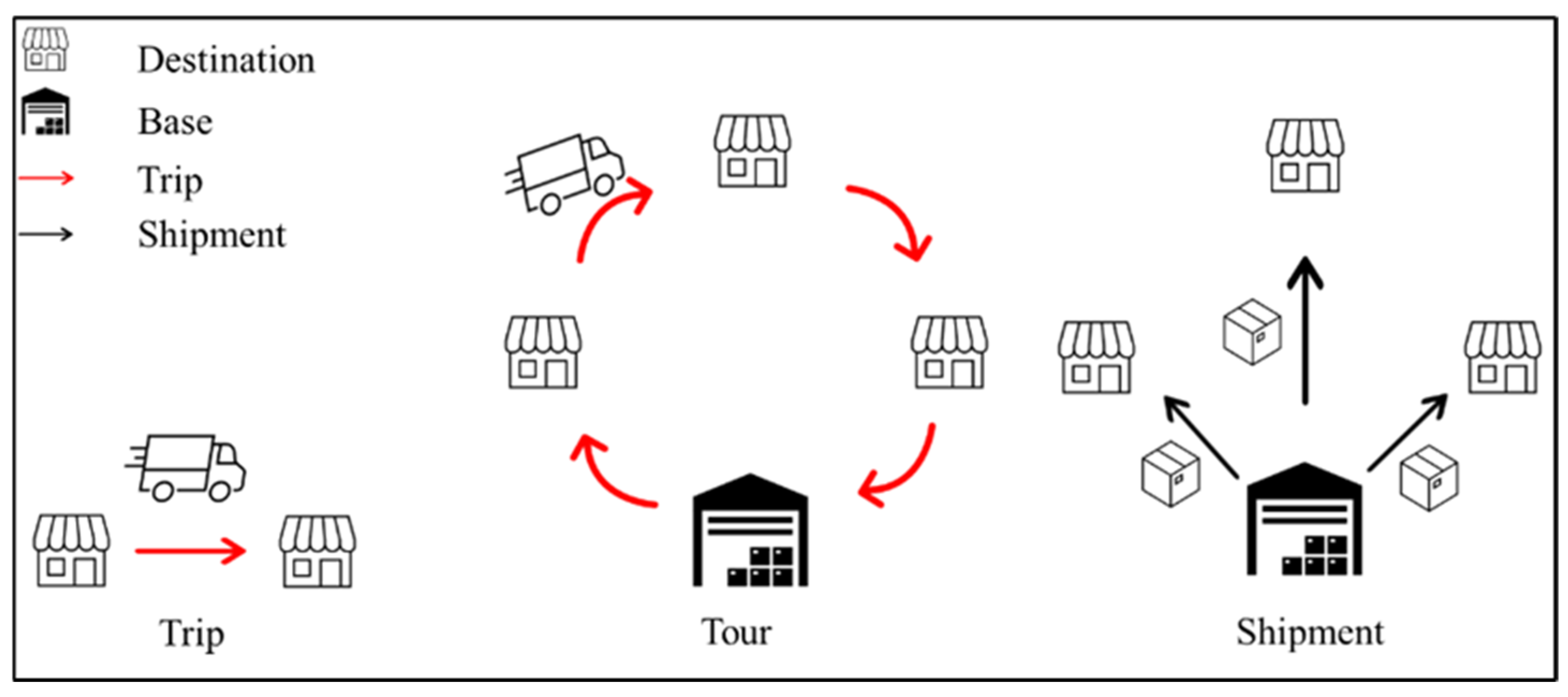
Readers must be aware that the terms used in this study are defined as follows (Figure 1): Base: the location where goods are loaded; Destination: the location where goods are delivered; Trip: movement between two stops by goods vehicle; Shipment: movement of goods from a base and a destination; Tour: a sequence of trips starting from a base and ending at the base or parking lot.
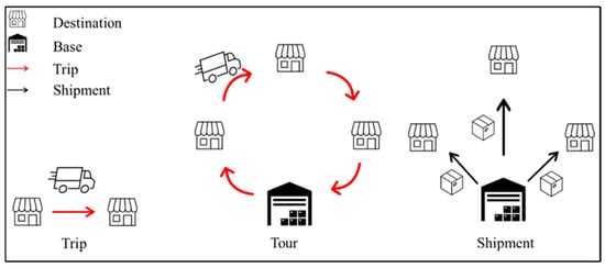
Figure 1.
Trips, tours, and shipments.
The rest of this paper consists of the following: Section 2 provides a review of the literature that focuses on modeling the shipment delivery time selection or vehicle tour start time and existing agent-based urban freight simulators; Section 3 provides an overview of the study area, the data we use, and how to generate pseudo-shipment records; Section 4 presents the specification of a delivery time-period selection model and the estimated model; Section 5 demonstrates the applicability of the model for replicating the observed delivery time distributions; and finally, Section 6 concludes the paper.
2. Literature Review
2.1. Selection Modeling of Delivery Time or Departure Time
Although there are many studies focusing on the time-of-day choice of passengers, to the best of our knowledge, only a handful papers have modeled delivery time selection. Delivery time choice has been discussed in the research of off-hour deliveries. For example, Holguin-Veras et al. [14] analyzed how different levels of tax deductions and shipping cost discounts affect the acceptance rate of off-hour deliveries by receivers. Holguin-Veras et al. [15] also analyzed the share of carriers that fulfill off-hour deliveries depending on a percentage of customers (receivers) requesting off-peak deliveries and incentives. Silas and Holguin-Veras [16] used the models developed by the above two studies and conducted policy simulations for the adoption of off-hour deliveries. Furthermore, Mepparambath et al. [17] conduced an establishment-based stated preference (SP) survey in Singapore. In their survey, they explain the characteristics of off-hour delivery or urban consolidation schemes, including delivery time (“during the night” or “next day morning”), and ask respondents if they are willing to participate in each of them. They collected the data from 95 shipper establishments and 80 stores in the retail district in Singapore and, like Holguin-Veras et al. [14], used it to estimate participation models for these schemes. Although these studies are insightful as to the prediction of the participation of off-hour delivery schemes by businesses, they give the limited insights regarding the heterogeneity of delivery time at the city scale due to their strong focus on retailers and restaurants in business districts and low granularity in the time periods considered.
In fact, de Jong et al.’s study [2] is the only study that analyzed the delivery time-period choice, considering detailed periods (7 periods). Noting the difficulty of collecting revealed preference (RP) data, they collected data using a SP survey and developed a delivery time-period choice model, aiming to use the model as a component of the Strategic Flemish Freight Model. They recruited logistics managers, purchase managers, or the directors from shipment receiving companies in the Flanders region, Belgium, and estimated multinomial logit (MNL) and mixed logit (ML) models, considering the transport time and cost using the data from 158 respondents. Due to the limited sample size, they considered only three categories of receivers: “producer”, “retailer”, and “wholesale, warehousing, distribution”, which underscores the need for an analytical approach that allows for large-scale data collection at a reasonable cost and effort. On the other hand, the advantage of their approach is that they collected the key policy variables such as transport time and cost. Their model and simulations using the model show that, under the situation where the receiver directly bears the cost, costs are very sensitive to the choice of time of day, although the transport time has a limited impact on the choice. Note that the data they used include long-distance shipments, which differs from our study focusing on the metropolitan scale.
There are more existing studies focused on vehicle departure times than delivery times, partially because the vehicle departure times are easier to obtain and a model simulating them is useful in cases where the simulation is not shipment-based but vehicle-based. Khan and Machemehl [12] used the commercial vehicle sample data collected in the 2006 Austin Commercial Vehicle Survey, conducted in Austin, Texas. They developed a multiple-discrete continuous probit (MDCP) model for predicting commercial vehicle time of day choice and vehicle use (i.e., vehicle miles traveled). Nadi et al. [13] proposed a model for vehicle routing and scheduling based on a parametrized time-dependent vehicle routing problem. The model is data-driven and aims to capture the spatial and temporal preferences of tour planners. To estimate the model parameters, they used a large tour database in the Netherlands that includes 16,171 tours implemented by 720 vehicles. While these two models are useful in many ways, they are limited in the sense that the selection of the time period to receive a shipment is not addressed and is substituted by the selection of the departure time for a vehicle, which is driven by different dynamics.
2.2. Agent-Based Urban Freight Simulators
In this subsection, we also briefly review urban freight simulation models that consider the shipment delivery time or vehicle departure time for traffic simulations, aiming to highlight the relevance of time-period choice models. Hunt and Stefan [5] proposed one of the earliest tour-based commercial vehicle movement models. Their model was calibrated using data from Calgary, Canada. They used observed tour start time distributions, considering carrier facility categories in tour generation. De Bok and Tavasszy [7] proposed an agent-based freight transportation model, MASS-GT, based on a large dataset of freight transportation collected by the Central Bureau of Statistics Netherlands. In this model’s freight delivery planning, the tour start time is assigned using the observed tour start time for each vehicle type and commodity type after assigning shipments to the tour. Therefore, this model does not consider the delivery time of each shipment in goods delivery planning. The two simulation models above require the distribution of tour start times as an input.
On the other hand, Nuzzolo et al. [4] proposed an urban freight demand modeling framework and demonstrated it using survey data from Rome, Italy. Their modeling framework includes a delivery time-period model, the output of which affects the number of tours generated in a given time period. However, in the implementation, the delivery time-period model is actually descriptive (i.e., a fixed probability is given for each time window). Similarly, SimMobility Freight (Sakai et al. [3]) defines delivery time windows, which become the conditions for vehicle operations planning (i.e., tour generation) during the simulation process, but uses the fixed probability distributions of delivery time windows defined by the commodity type. Thus, in the case of Nuzzolo et al. [4] and Sakai et al. [3], the framework is designed to accommodate a delivery time-period selection model, but the model has not been estimated for them. Stinson et al. [18] proposed another agent-based model called CRISTAL. They solved a service time-constrained vehicle capacitated routing problem (STC-VRP) for tour generation, but the details are not available in the paper, and we could not confirm the use of shipment delivery time or vehicle departure time.
2.3. Research Gap
Despite the growing need for the simulation of delivery times for policy analysis and the fact that state-of-the-art urban freight simulation models require delivery time information (or alternatively, tour start time information) in the simulation process, to the best of our knowledge, only de Jong et al. [2] studied shipment delivery time modeling considering alternative time periods that were detailed enough for the simulation models. As we mentioned in the introduction, we address this research gap by proposing an approach using GPS data for generating pseudo-shipment records with delivery time-period information, estimating a shipment delivery time model, and obtaining insights from the estimated model.
3. Data
3.1. Study Area
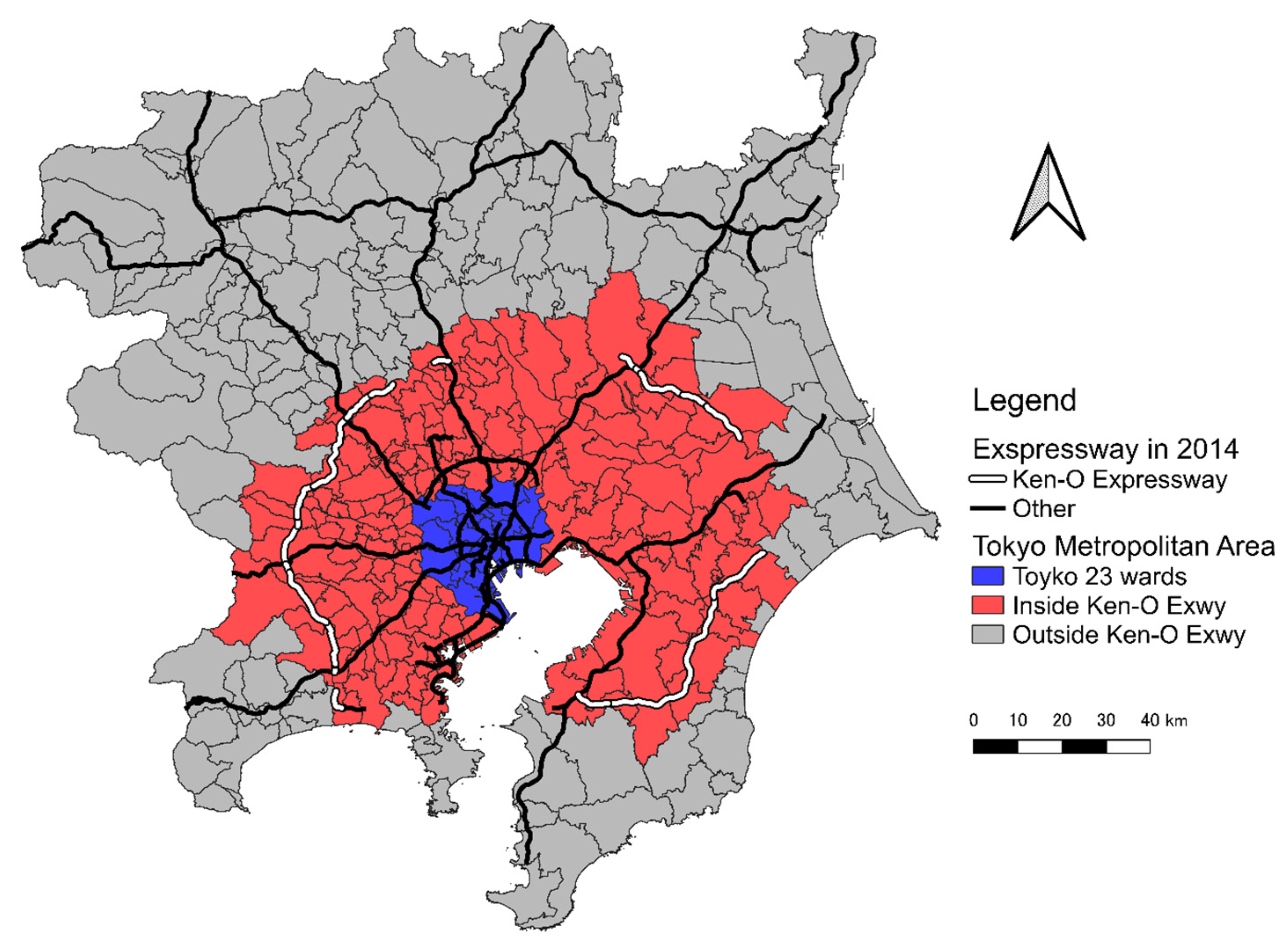
The present study focuses on intra-metropolitan shipments, the origins and destinations of which are in the TMA (Figure 2). The study area covers 22.2 thousand km2, accounting for only 5.8% of Japan’s total land area but having a population of approximately 42.8 million (33.9% of Japan’ total population). Furthermore, many large factories and logistics facilities are located in the study area, especially along the expressway network, which significantly contribute to intra-city traffic. According to the 2013 Tokyo Metropolitan Freight Survey (TMFS) [19]), the intra-city freight flow is about 2.8 million tons per day. Moreover, Tokyo is a port city and a transportation hub and has one of the largest industrial regions in the nation. There are two of Japan’s largest international airports, Tokyo International Airport in Ota Ward, Tokyo Prefecture, and Narita International Airport in Narita City, Chiba Prefecture, one of Japan’s largest freight railway terminals, Tokyo Freight Terminal Station in Shinagawa Ward, Tokyo, and large-scale container terminals along Tokyo Bay. According to the TMFS, the external inbound and outbound freight flows are 801 and 823 thousand tons per day, respectively.
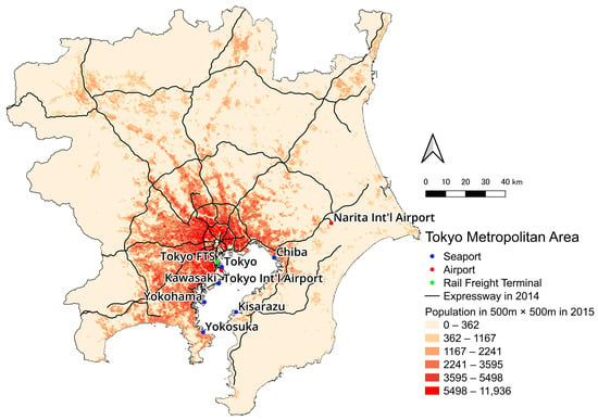
Figure 2.
Tokyo Metropolitan Area.
3.2. GPS Data
We used GPS data, which include vehicle trajectory data (time and location), obtained through the cloud-based operation management system “MIMAMORI”. The data were originally collected by Isuzu Motors Limited [20], the largest goods vehicle manufacturer in Japan, with a 36% market share in Japan in 2022 and made available for us by the Transportation Planning Commission of the Tokyo Metropolitan Region. MIMAMORI is one of the major vehicle operation management services in Japan, and its trajectory accuracy is considered high enough for this study. The data include information on the geographic coordinates, date, time, and type of goods vehicle, and are collected every 10 min unless the driver turns off the engine. Dead zones and electromagnetic jammers are common concerns in analyses using GPS data. However, since this study focuses on the “stop” portion (for loading and unloading) rather than the moving portion, these issues are less concerning. It should be noted that, like many other raw GPS data on goods vehicle trajectories available elsewhere, these data do not include information such as the type of goods transported and stop purposes (e.g., loading, unloading, and in-transit); a costly complementary driver survey is needed to collect this information (Ben-Akiva et al. [10]; Alho et al. [21]). The data include four types of goods vehicles: (1) large-size tractor, (2) large-size truck, (3) medium-size truck, and (4) small-size truck. According to the Ministry of Land, Infrastructure, Transport and Tourism (MLIT) [22], Isuzu Motors Limited classifies vehicles based on engine displacement. Large-size vehicles (tractors or trucks) are those with an engine displacement of 8000 cc or more. Medium-size trucks have an engine displacement between 3000 cc and 7999 cc, and small-size trucks have an engine displacement of 3000 cc or less. The number of vehicles by vehicle type is 528, 5518, 12,324, and 8860, respectively. We use the data of vehicles that started their operations on Monday, 6 October, and Tuesday, 7 October 2014. We consider that the data might be a little out of date, but the delivery time mechanism for business establishments in general should not have changed dramatically in a decade or so. For example, for decades in Japan, grocery stores have tended to receive goods early in the morning to restock before opening. Furthermore, major parcel delivery service providers operate some hub facilities 24 h a day (e.g., Yamato Holdings’ Haneda Chronogate was completed in 2013 and is still in operation as of the end of 2024 [23]). To the best of our knowledge, there is no literature that indicates any significant changes in the delivery time mechanism for specific shipment types in Tokyo or Japan over the past decade. This is not to say that the distribution of delivery times has been entirely stable over this period, but the data can be considered recent enough to capture an abstraction of long-lasting delivery time characteristics.
3.3. Tours and Shipments
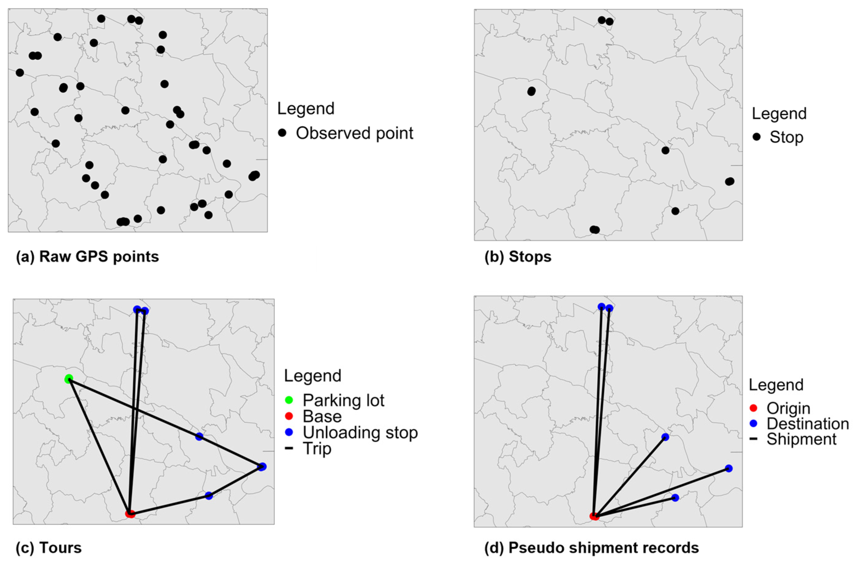
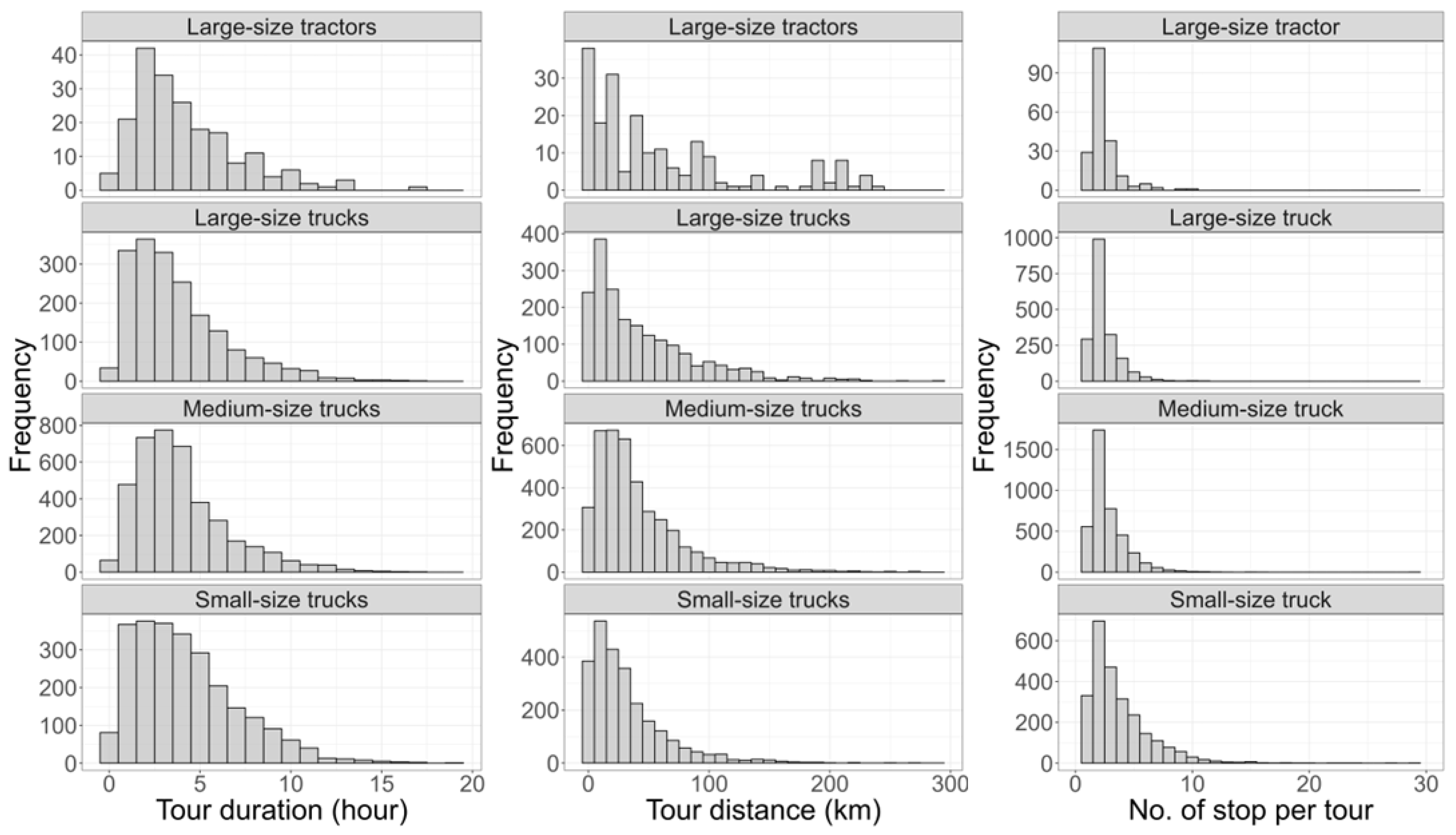
The vehicles in the dataset were assumed to be on a delivery tour, and the origin and destination of the shipment were inferred based on the trajectory of the goods vehicle. An example of raw GPS point data is shown in Figure 3a. Data processing was performed as follows. (1) Points with a Euclidean distance of less than 500 m from the last observed point were considered as “stops” (Figure 3b), following the method used by Romano Alho et al. [21]. The time difference between the first and last points at each stop location was computed as the stop duration. (2) Stops equal to or longer than 300 min were considered as prolonged parking for operational breaks in parking lots (e.g., overnight parking). The 300-minute period was selected because, based on the 2021 Road Traffic Census data provided by the MLIT, about 92% of the loading/unloading stops by goods vehicles are equal to or less than 300 min. Stop sequences were divided by the prolonged parking and each resulting stop sequence was referred to as an “operation”. Note that only operation data of less than 24 h were used. (3) For each operation, trips were generated by connecting stops in sequence. The first trip of each operation is considered the trip from a parking lot to a base where goods are presumed to be loaded. The other stops were considered as unloading stops. We used the data of operations in which goods vehicles have returned to their base at least once (Figure 3c). A stop sequence that starts from a base and ends at a base or a parking lot is referred to as a “tour”. The distributions of tour distance (sum of Euclidean distances for trips in the tour), tour duration, and number of stops (base and destination) in a tour are shown in Figure 4. The figure shows that, while there is no significant difference in the duration for each goods vehicle type, the smaller the vehicle, the more stops each tour makes, and the larger the vehicle, the longer the tour distance. (4) Pseudo-shipment records were created by treating the loading stop locations (i.e., base) as shipment origins and unloading stop locations as shipment destinations (Figure 3d). Table 1 shows the numbers of vehicles, tours, and pseudo shipments in the final dataset, by vehicle type.
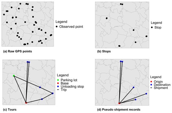
Figure 3.
Visualization of the data processing flow. (a) raw GPS points; (b) stops; (c) tours; and (d) pseudo shipment records.

Figure 4.
Tour characteristics by vehicle type.

Table 1.
Numbers of vehicles, tours, and pseudo shipments.
3.4. Goods Type
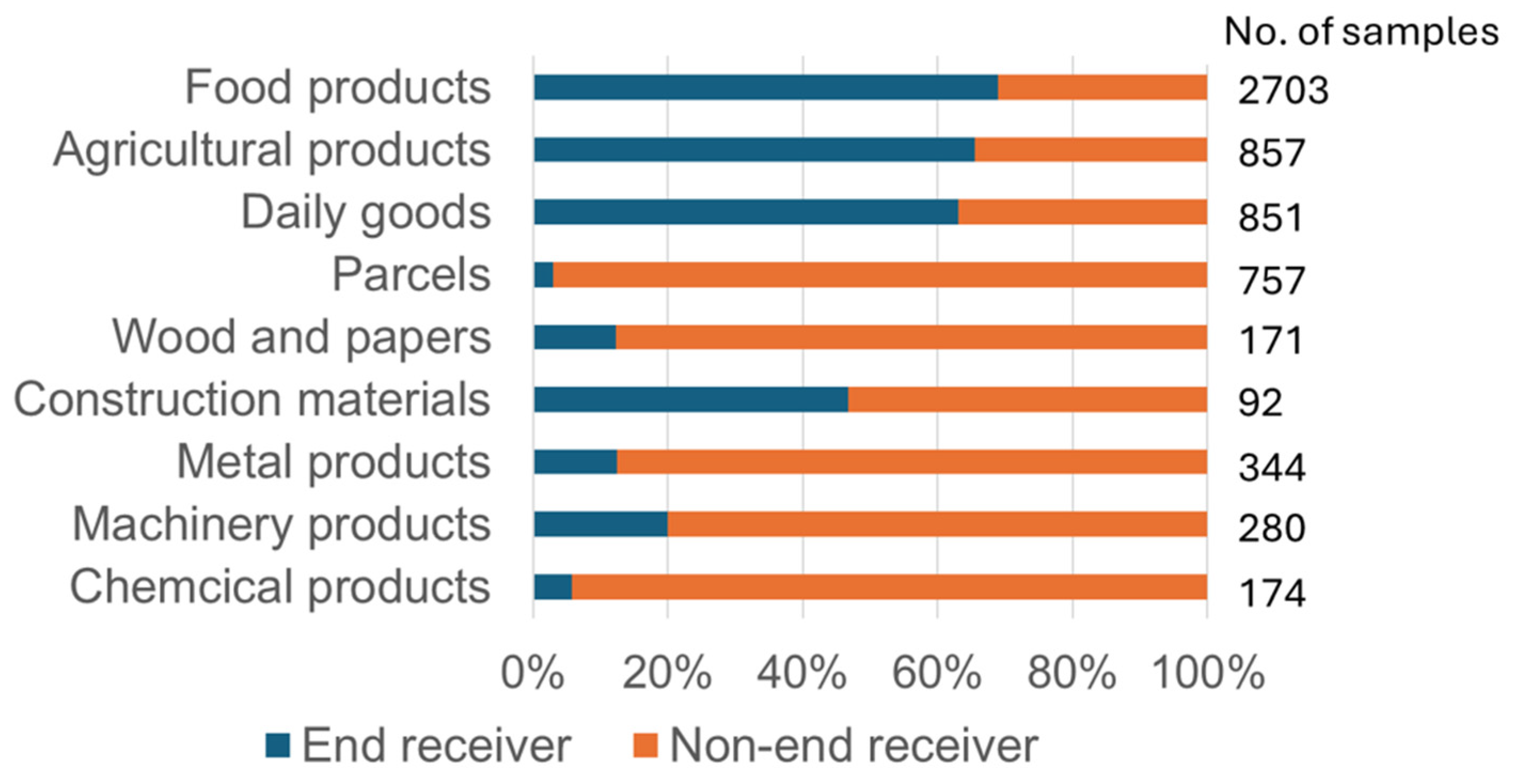
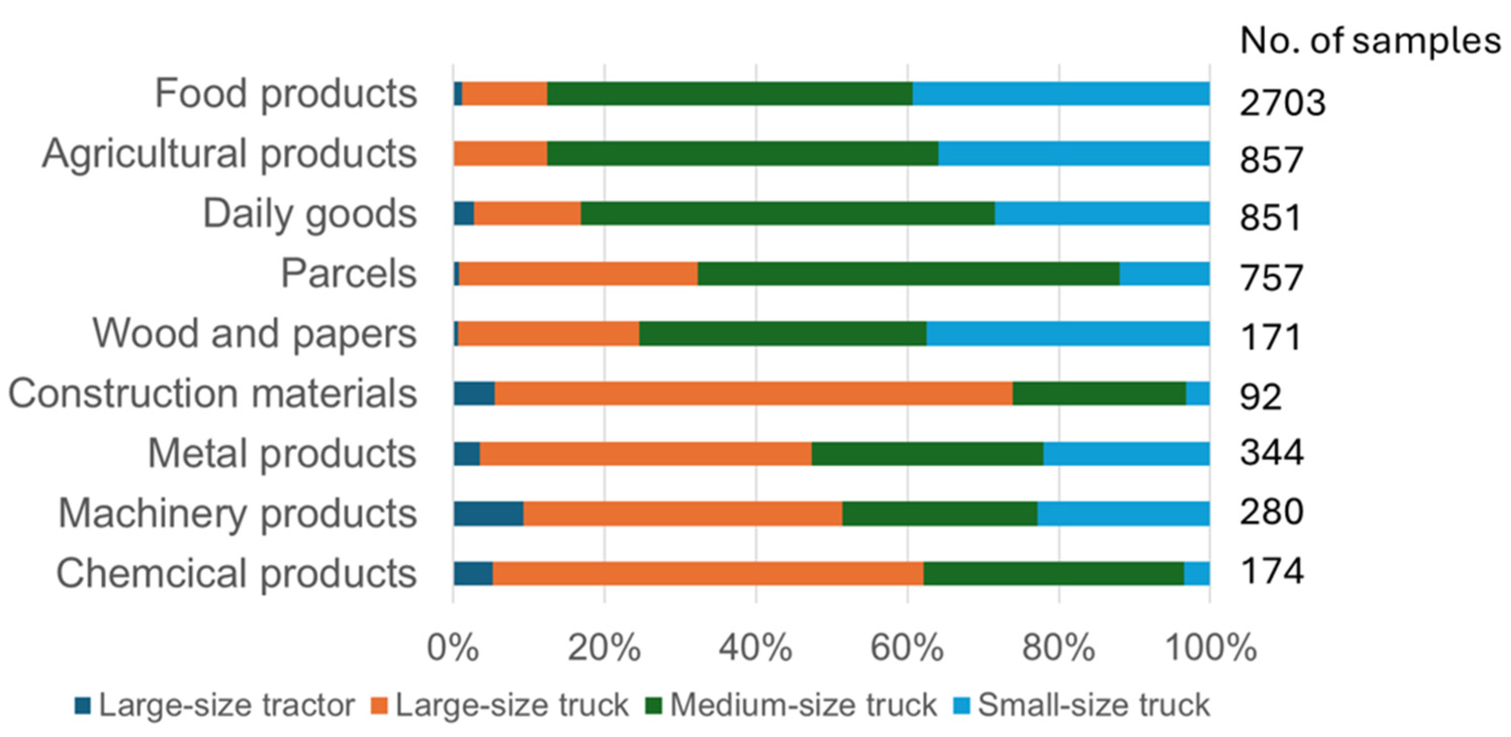
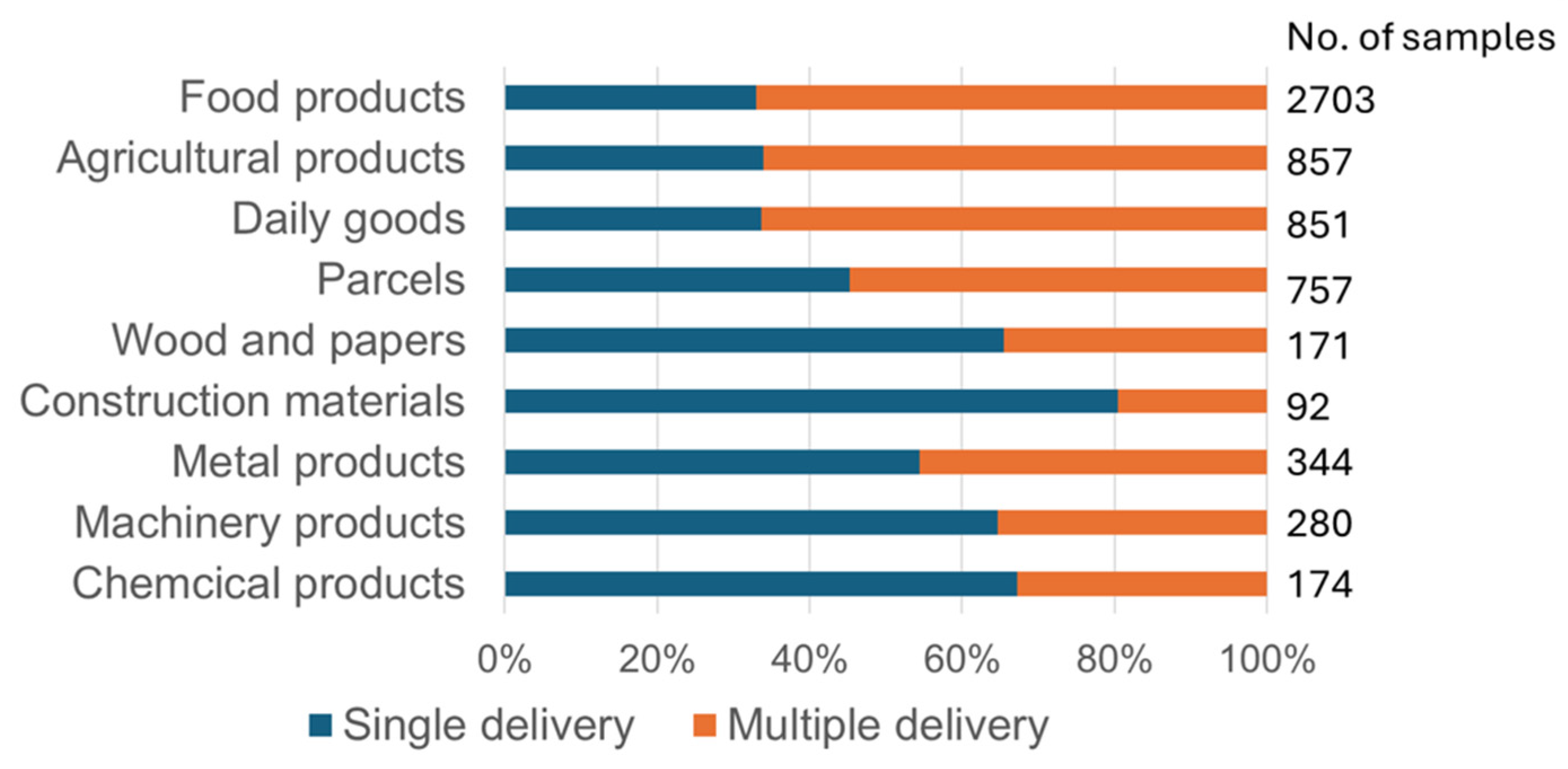
As mentioned earlier, our data do not include the type of goods transported. To infer the type of goods, Google Maps was used to identify the business types of stops (bases and destinations). Since the data are from 2014, the aerial photographs in Google Maps available today may differ from those at that time. To obtain more accurate data, Google Maps Street View [24] and Denshikokudo Web System [25] provided by Geospatial Information Authority of Japan were used. The former provides past street views, and the latter provides aerial photographs of the area in the past. Also, if available, the websites of the establishments at the stops were checked to collect information of the type of handled goods (e.g., food products warehouse). The above process could be replaced by the use of Point-of-Interest (POI) data, which were not available for this study, and spatial matching of stops with POIs. We used this information to assign (inferred) shipments to one of the following nine goods type categories: (1) food products (e.g., beverages, seasonings, and processed food), (2) agricultural products (e.g., vegetables, feeds, and milk), (3) daily goods (e.g., clothes, medicines, and cosmetics), (4) parcels, (5) wood and papers (e.g., square timbers, paper, and books), (6) construction materials (e.g., concrete, stone, and glass), (7) metal products (e.g., metal parts, iron plates, and steel pipes), (8) machinery products (e.g., cars, dental equipment, and appliances) and (9) chemical products (e.g., plastics, plastic pipes, and rubber). The following rule was used to assign the type of goods to shipments: if the goods type handled by the base establishment is apparent, assign that goods type; otherwise, if the goods type handled by the destination establishment is apparent, assign that goods type. Shipments that are difficult to categorize by goods type, such as shipments between warehouses of general logistics companies that handle different items, were excluded. Note that “parcels” were assigned to shipments from the establishments of the largest delivery service providers in Japan, Sagawa Express, Yamato Transport, and Japan Post. Furthermore, the stops are classified into four business type categories: (1) end receiver, (2) warehouse, (3) factory, and (4) others. “End receiver” refers to the location where the goods are consumed or purchased, such as retail stores, offices, construction sites, and restaurants; the other three business types are also referred to as “non-end receiver”. Figure 5 shows whether the receiver is an “end receiver” for each goods type. “Food products”, “agricultural products”, and “daily goods” are often destined for “end receivers”. These three types of products also exhibit similar characteristics with respect to the vehicle type used (Figure 6) and whether the shipment is implemented by a single or multiple delivery tour (Figure 7).

Figure 5.
Share of shipments sent to end receivers for each goods type.
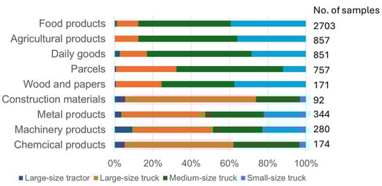
Figure 6.
Share of shipments by vehicle type used for each goods type.
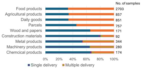
Figure 7.
Share of shipments by tour type used for each goods type.
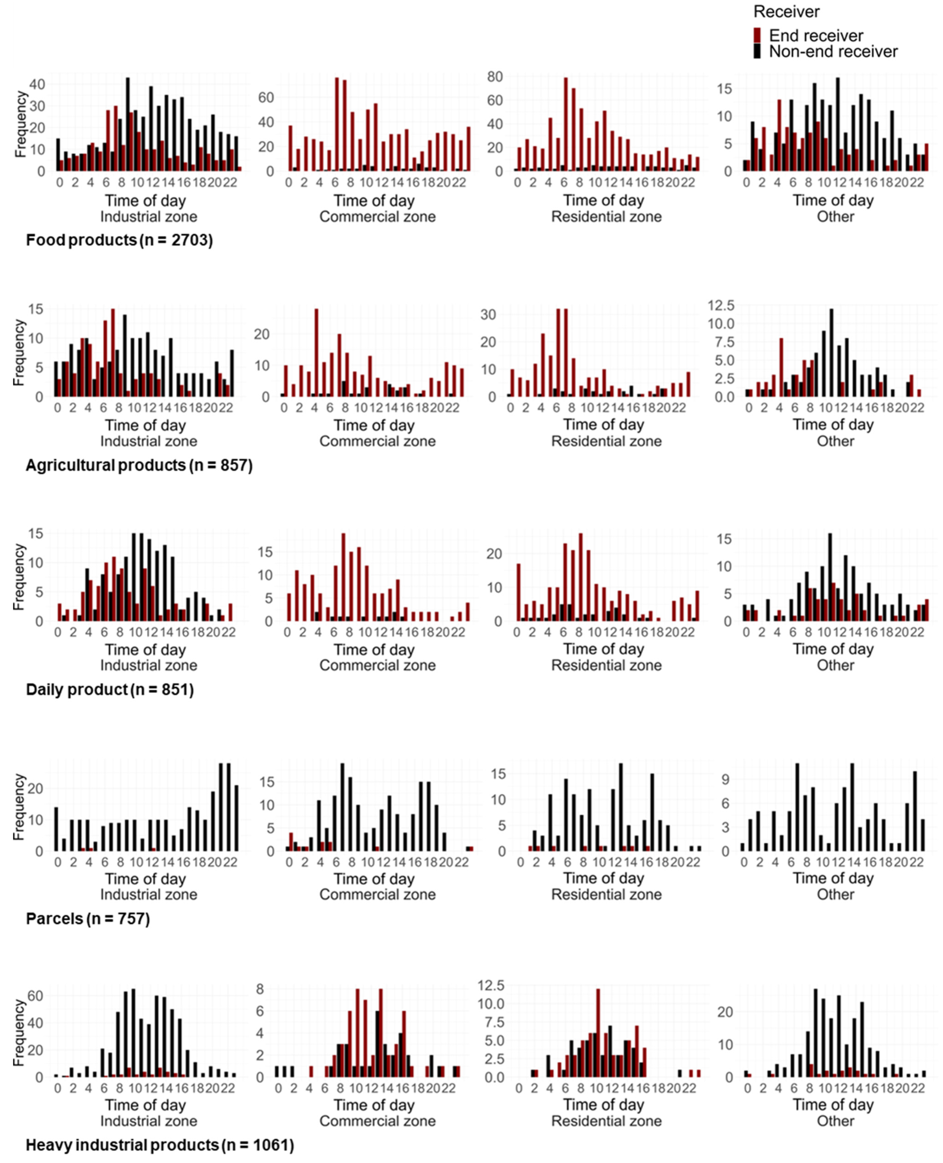
In the following analysis, “wood and papers”, “construction materials”, “metal products”, “machinery products”, and “chemical products” are grouped together as “heavy industrial products”. Figure 8 shows the distribution of the number of shipments received by time of day, the type of goods, and whether the receiver is an “end receiver”. The figure shows that “end receivers” of “food products” receive goods mostly between 6 a.m. and 8 a.m. On the other hand, “non-end receivers” tend to receive shipments more evenly throughout the day, although there are peaks during the day. As for “agricultural products”, “end receivers” receive goods intensively between midnight and morning and rarely in the afternoon and evening, while the delivery time distribution of “non-end receivers” has no clear peaks. For “daily goods”, the peaks are from 6–9 a.m. and from 11 p.m.–1 a.m. With respect to shipments to “non-end receivers”, unlike the previous two types of goods, goods are mostly received between 6 a.m. and 3 p.m. In “parcels”, there are few shipment samples to “end receivers”; most of them are received at convenience stores after midnight. This is because some convenience stores, which are open 24 h a day, affiliate with delivery service providers and serve as pick-up and drop-off points. Moreover, the delivery time distribution of shipments to “non-end receivers” is completely different from the other goods types. The data highlight the characteristics of operations by the delivery service providers. In “heavy industrial products”, there appears to be no difference in the distribution of the number of receiving goods by “end receivers”/“non-end receivers”. The distribution itself resembles that of “daily goods” shipments to “non-end receivers”, with most deliveries occurring during the day. In short, for any type of goods except for “heavy industrial products”, goods to “end receivers” tend to be received from midnight to morning. This might be because end receivers such as retail shops and restaurants should receive shipments before the opening hours to complete the display of goods or prepare for service.
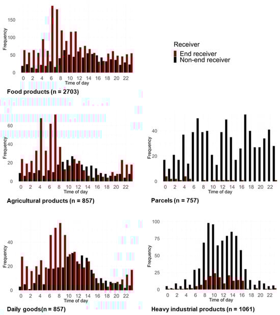
Figure 8.
Delivery time of day distributions.
3.5. Zoning Type of Destination
The influence of the zoning type of the shipment’s destination on the goods delivery time selection was also analyzed, using the zoning type data available from the national archives (MLIT [26] and MLIT [27]). We combined detailed zoning types into four zoning categories: industrial zone (quasi-industrial, industrial, and exclusively industrial), commercial zone (neighborhood commercial and commercial), residential zone (Category I exclusively low-rise residential, Category II exclusively low-rise residential, Category I mid/high-rise oriented residential, Category II mid/high-rise oriented residential, Category I residential, Category II residential, and Quasi-residential), and others (urbanization control area and outside of city planning area). Figure 9 shows the distribution of the number of shipments received by the time of day by goods and zoning types. In the “industrial zone”, “parcels” shipments tend to be received late at night. In contrast, in “residential” and “commercial zones”, “parcels” are received in the morning or evening. This should be due to differences in the functions of establishments that are associated with zoning types. For the other goods type, we did not observe clear differences in delivery times by zoning type.
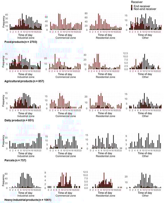
Figure 9.
Delivery time of day by zoning type.
3.6. Pseudo-Shipment Size
Our pseudo-shipment records do not have information on shipment size. Therefore, we compute the pseudo-shipment size of shipment i using Equation (1) below:
where is the no. of stops at destinations of the tour that fulfilled shipment i; is the load capacity of vehicle size assigned to shipment i; and is the load factor (=0.73).
We use the average load capacities of vehicles sold by Isuzu Motors in 2014 [22]. The average load capacities are 27,097 kg for a large-size tractor, 14,480 kg for a large-size truck, 7142 kg for a medium-size truck, and 2477 kg for a small-size truck. The load factor is calculated using Equation (2) below:
where TKFT refers to the ton-kilometers of freight transported and TKTC refers to the ton-kilometers of the transport capacity. Both of those variables are based on the Survey on Motor Vehicle Transport 2014 (MLIT [28]).
4. Method: Model Description
For understanding the factors that affect shipment delivery time periods and the degrees of their effects, as well as for developing a simulation model for future use, we estimate the delivery time selection models. The variables used are summarized in Table 2. For “heavy industrial products”, we could not use zoning types because most of the shipment’s destinations are in an “industrial zone” or “other”. Instead, we consider detailed goods categories for “heavy industrial products”: “metal products”, “machinery products”, “chemical products”, and “others”. Note that our models do not include any cost relevant variables since the data of such variables are not available for us, which is the limitation of our approach relying on GPS data. We do not include information on tours to fulfill shipments, since we consider the delivery time (or time period) as a prerequisite to be considered in planning vehicle operations and deliveries.
Table 2.
Definitions of variables.
We develop the multinomial logit model and estimate the model parameters using the maximum likelihood estimation method. The utility of an alternative delivery time period j for shipment i, , consists of a systematic component and a randomly distributed unobserved component, which is as shown in Equation (3) below:
where is an observed systematic component and is a randomly distributed unobserved component that follows a Gumbel distribution with scale = 1 and location = 0. The observed systematic component is specified as follows: Equation (4) is used for “food products”, “agricultural products”, “daily goods”, or “parcels”, while Equation (5) is for “heavy industrial products”.
The base category of the choice alternative is “morning”. , , , , , , , , , and are the parameters to be estimated. Equation (6) shows the probability that, given the set of alternative time periods , delivery time period is selected for shipment .
The parameters are estimated using the maximum likelihood estimation (Equation (7)). Note that is the set of parameters to be estimated and is the set of samples (i.e., shipments).
5. Results
The estimated models are shown in Table 3, Table 4, Table 5, Table 6 and Table 7. The results show that the longer the shipment distance, the more likely the time periods of “night”, “late at night”, and “early morning” are selected (coefficients of ln_dist for “night”, “late at night”, and “early morning” are all positive), and many shipment distance coefficients of “night”, “late at night”, and “early morning” are statistically significant. Long-distance shipments are less likely to be received during the day (“morning” and “afternoon”), potentially because of heavy traffic, which leads to higher transportation costs and unstable arrival times. Especially for “parcels”, the coefficient of ln_dist for “late at night” is high (0.649). This result may be attributed to the fact that the parcel delivery service industry transports their goods at night between regional hubs far from each other.
Table 3.
Estimated goods delivery time selection model (food products).
Table 4.
Estimated goods delivery time selection model (agricultural products).
Table 5.
Estimated goods delivery time selection model (daily goods).
Table 6.
Estimated goods delivery time selection model (parcels).
Table 7.
Estimated goods delivery time selection model (heavy industrial products).
As for the shipment size, if shipments are “daily goods”, “parcels”, or “heavy industrial products”, large shipments are less likely to be received during the day, and almost all coefficients of ln_size for “night”, “late at night”, and “early morning” are statistically significant. Small establishments receive small shipments, often only during their business hours, while large factories and logistics facilities that handle large amounts of goods receive large shipments even “late at night”. Large facilities would have more employees and would be able to assign employees during night-time. Furthermore, for “parcels”, the coefficient of ln_size for “late at night” is especially high (1.270). This reflects the fact that facilities handling shipments of different sizes have different functions in parcel logistics. In parcel delivery services, small facilities often serve as microhubs and handle small shipments during the daytime, while large facilities serve as regional hubs and receive large, consolidated shipments at night. On the other hand, for “food products” and “agricultural products”, which are perishable goods, the larger the shipments are, the more likely they are received during the day, especially in the “afternoon”. In general, perishable goods should be distributed from producers to consumers in a shorter period of time than other types of goods, which should explain the difference in coefficients between these two goods types and the others.
Furthermore, for “agricultural products”, “daily goods”, and “parcels”, the coefficients of dum_endr for “late at night” are positive and statistically significant. While the coefficient for “early morning” shows a higher coefficient for “agricultural products” (1.791), those for “late at night” are highest for “daily goods” and “parcels”. This is an interesting finding in relation to policies that encourage off-hour deliveries. In fact, many of the end receiver businesses (retail stores, offices, construction sites, and restaurants) in the study area receive goods at night and this is observed in the models even after controlling for the variables (such as shipment size and distance) we consider. According to Holguin-Veras et al. [14], the main reason for receivers not to receive deliveries during night-time is that they are not open during that time. On the other hand, there are many stores that open during night-time in the TMA, especially in the business districts. Therefore, the burden of night-time delivery may be low. According to the 2021 Economic Census (Ministry of Economic, Trade and Industry [29]), 23.5% of the establishments that serve food and beverages in Tokyo are open 24 h, and 39.2% of them are open more than 14 h. For “food products”, the coefficient of dum_endr is highest and statistically significant for “early morning” (0.690). Grocery stores need to receive goods before or at the time of opening their shops to display goods (Nuzzolo et al. [4]).
Although we expect that zoning types have an effect on delivery time for “parcels”, as mentioned in the prior section, almost all parameters are statistically insignificant. This highlights the importance of shipment-specific characteristics instead of district-level characteristics. The dummy variables for “end receiver”, “chemical”, “machinery”, and “metal” (, , , and ) are all insignificant for “heavy industrial products”.
In summary, the estimated coefficients reflect the supply chain characteristics of different types of goods, which is especially clear for “parcels”, and also reflect the adoption of deliveries during night-time. The estimated models show their potential for the realistic replication of delivery times when used for freight simulation. Also, the presented modeling analysis indicates that the pseudo-shipment data can be used to analyze the delivery time periods with theoretically reasonable directions of effects. However, the rho-squared values (pseudo-R2) are relatively low. Therefore, to investigate the practicality of the modeling approach, we apply the model to areas in the TMA with different land use characteristics and examine whether the model could reproduce the differences in delivery time periods among these areas.
6. Additional Analysis: Demonstrative Application
For demonstrating the capability of the model, the TMA is divided into three areas, as shown in Figure 10, and the estimated models are used to replicate the delivery time periods in those areas. The characteristics of each area and the number of sample shipments received at each area are as follows:

Figure 10.
The three areas considered in the demonstration.
Tokyo 23 wards: The central core of the TMA, where many business districts are located, and businesses and retailing are most active. The number of sample shipments received in this area is 1613.
Inside Ken-O Exwy: The area inside the Ken-O Expressway, the 3rd ring road, excluding “Tokyo 23 wards”. A large part of the area is residential, and many of the Tokyo 23 wards’ workers commute from there. The number of sample shipments received in this area is 3455.
Outside Ken-O Exwy: The area outside of the Ken-O Expressway. The area is generally suburban and exurban. Furthermore, because land prices are low and land is readily available, many heavy industrial and logistics facilities are located in this area. The number of sample shipments received in this area is 1161.
The types of goods and receivers of sample shipments by area are shown in Table 8. Note that the data used for this demonstrative application are the same as those used for the model estimation. In the Tokyo 23 wards, the share of “end receivers” is much higher than that of “non-end receivers”, but the opposite is true outside the Ken-O Exwy.
Table 8.
Goods type and receiver type of sample shipments by received area.
We simulate the delivery time period for each shipment sample 1000 times and compute the average of the count of selections for each alternative. Then, we aggregate the results and compare them with the observed counts, as shown in Figure 11 and Table 9. The figure and the table indicate that the distribution of simulated counts closely matches the observed distribution. The models accurately capture the characteristics of each district. In the Tokyo 23 wards, where consumption activity is concentrated, the receiving of goods is concentrated during “early morning” and “late at night”. In the Outside Ken-O Exwy area, where many “heavy industrial products” are delivered, the receiving of goods is concentrated during the day, especially in the “afternoon”. As for the Inside Ken-O Exwy area, the distribution of delivery time periods is somehow intermediate between Tokyo 23 wards and Outside Ken-O Exwy. The simulation result is closest to the observed distribution for Inside Ken-O Exwy.
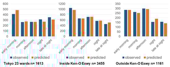
Figure 11.
The comparison of observed and predicted delivery time periods.
Table 9.
The comparison of the share of observed and predicted receiving of goods.
7. Conclusions
We generated pseudo-shipment data by processing GPS vehicle trajectory data and then developed goods delivery time-period selection models for different goods types. The models consider the information about the shipment, which consists of the following variables: (1) the distance between the shipment’s origin and destination, (2) shipment size, which is calculated based on load capacity, number of stops in a tour, and average load factors, (3) attributes of destination such as establishment’s function and zoning type of its location, and (4) inferred goods types. We found that long-distance shipments are likely to be received during night-time or early morning. Also, non-perishable large shipments are less likely to be received during the day (“morning” or “afternoon”). This especially applies to the parcel delivery service industry, reflecting its unique logistical characteristics. On the other hand, large perishable goods (“food” or “agricultural products”) are likely to be received during the day. Goods to end receivers (such as stores and restaurants) are more likely to be delivered “late at night” or “early morning”, although this does not apply to “heavy industrial goods”. This finding is likely related to the fact that many of the stores and restaurants in the TMA are open for longer hours per day. We also demonstrated the practicality of the models by comparing the simulation result with the observed data for three areas with distinct characteristics and confirmed that the model can accurately replicate goods delivery time-period distributions, which is critically important for freight demand analysis, as appropriate policy measures depend on the time of day when demand occurs. We conclude that the model estimated by the proposed approach would be applicable to urban freight simulation models, including the state-of-the-art agent-based models, to accurately reproduce spatial heterogeneity in shipment delivery time periods.
Noting the limitation of our research, because of the difficulty in obtaining the relevant information, our estimated model does not include cost-related variables, which is a significant limitation in the model. The past studies (Holguin-Veras et al. [30]; Holguin-Veras [31]; de Jong et al. [2]) indicate that the cost sensitivity is different depending on whether transportation costs are directly imposed on receivers, and it is desirable for the model to have sensitivity to costs under different transport contract settings. With its cost sensitivity, the model is expected to be more useful to simulate and evaluate various policies. The addition of such cost sensitivities to our model specification, exploring the use of publicly available data, is left to future research.
Author Contributions
Conceptualization, T.S.; methodology, R.K. and T.S.; formal analysis, R.K.; writing—original draft preparation, R.K. and T.S.; writing—review and editing, T.S. and T.H.; visualization, R.K.; supervision, T.S. and T.H. All authors have read and agreed to the published version of the manuscript.
Funding
This work was supported by JSPS KAKENHI Grant Number 23K13421.
Data Availability Statement
The datasets presented in this article are not readily available because the Transport Planning Commission of the Tokyo Metropolitan Region shares the datasets with restrictions on their use. Requests to access the datasets should be directed to the Transport Planning Commission of the Tokyo Metropolitan Region.
Acknowledgments
We would like to thank the Transport Planning Commission of the Tokyo Metropolitan Region for sharing the data for this research.
Conflicts of Interest
The authors declare no conflicts of interest.
References
- Holguín-Veras, J.; Leal, J.A.; Sánchez-Diaz, I.; Browne, M.; Wojtowicz, J. State of the art and practice of urban freight management: Part I: Infrastructure, vehicle-related, and traffic operations. Transp. Res. Part A Policy Pract. 2020, 137, 360–382. [Google Scholar] [CrossRef]
- De Jong, G.; Kouwenhoven, M.; Ruijs, K.; van Houwe, P.; Borremans, D. A time-period choice model for road freight transport in Flanders based on stated preference data. Transp. Res. Part E Logist. Transp. Rev. 2016, 86, 20–31. [Google Scholar] [CrossRef]
- Sakai, T.; Alho, A.R.; Bhavathrathan, B.K.; Dalla Chiara, G.; Gopalakrishnan, R.; Jing, P.; Ben-Akiva, M. SimMobility Freight: An agent-based urban freight simulator for evaluating logistics solutions. Transp. Res. Part E Logist. Transp. Rev. 2020, 141, 102017. [Google Scholar] [CrossRef]
- Nuzzolo, A.; Comi, A. Urban freight demand forecasting: A mixed quantity/delivery/vehicle-based model. Transp. Res. Part E Logist. Transp. Rev. 2014, 65, 84–98. [Google Scholar] [CrossRef]
- Hunt, J.D.; Stefan, K.J. Tour-based microsimulation of urban commercial movements. Transp. Res. Part B Methodol. 2007, 41, 981–1013. [Google Scholar] [CrossRef]
- Nadi, A.; Yorke-Smith, N.; Snelder, M.; Van Lint, J.W.C.; Tavasszy, L. Data-driven preference-based routing and scheduling for activity-based freight transport modelling. Transp. Res. Part C Emerg. Technol. 2024, 158, 104413. [Google Scholar] [CrossRef]
- De Bok, M.; Tavasszy, L. An empirical agent-based simulation system for urban goods transport (MASS-GT). Procedia Comput. Sci. 2018, 130, 126–133. [Google Scholar] [CrossRef]
- Oka, H.; Hagino, Y.; Kenmochi, T.; Tani, R.; Nishi, R.; Endo, K.; Fukuda, D. Predicting travel pattern changes of freight trucks in the Tokyo Metropolitan area based on the latest large-scale urban freight survey and route choice modeling. Transp. Res. Part E Logist. Transp. Rev. 2019, 129, 305–324. [Google Scholar] [CrossRef]
- Tok, A.; Hyun, K.; Hernandez, S.; Jeong, K.; Sun, Y.; Rindt, C.; Ritchie, S.G. Truck Activity Monitoring System for Freight Transportation Analysis. Transp. Res. Rec. 2017, 2610, 97–107. [Google Scholar] [CrossRef]
- Ben-Akiva, M.E.; Toledo, T.; Santos, J.; Cox, N.; Zhao, F.; Lee, Y.J.; Marzano, V. Freight data collection using GPS and web-based surveys: Insights from US truck drivers’ survey and perspectives for urban freight. Case Stud. Transp. Policy 2016, 4, 38–44. [Google Scholar] [CrossRef]
- Stefan, K.J.; McMillan, J.D.P.; Hunt, J.D. Urban commercial vehicle movement model for Calgary, Alberta, Canada. Transp. Res. Rec. 2005, 1921, 1–10. [Google Scholar] [CrossRef]
- Khan, M.; Machemehl, R. Commercial vehicles time of day choice behavior in urban areas. Transp. Res. Part A Policy Pract. 2017, 102, 68–83. [Google Scholar] [CrossRef]
- Nadi, A.; Tavasszy, L.; van Lint, J.W.C.; Snelder, M. Spatial and Temporal Characteristics of Freight Tours: A Data-Driven Exploratory Analysis. arXiv 2023, arXiv:2311.15287. [Google Scholar]
- Holguín-Veras, J.; Silas, M.; Polimeni, J.; Cruz, B. An Investigation on the Effectiveness of Joint Receiver–Carrier Policies to Increase Truck Traffic in the Off-peak Hours. Part I: The Behavior of Receivers. Netw. Spat. Econ. 2007, 7, 277–295. [Google Scholar] [CrossRef]
- Holguín-Veras, J.; Silas, M.; Polimeni, J.; Cruz, B. An Investigation on the Effectiveness of Joint Receiver–Carrier Policies to Increase Truck Traffic in the Off-peak Hours: Part II: The Behavior of Carriers. Netw. Spat. Econ. 2008, 8, 327–354. [Google Scholar] [CrossRef]
- Silas, M.A.; Holguín-Veras, J. Behavioral microsimulation formulation for analysis and design of off-hour delivery policies in urban areas. Transp. Res. Rec. 2009, 2097, 43–50. [Google Scholar] [CrossRef]
- Mepparambath, R.M.; Cheah, L.; Zegras, P.C.; Alho, A.R.; Sakai, T. Evaluating the impact of urban consolidation center and off-hour deliveries on freight flows to a retail district using agent-based simulation. Transp. Res. Rec. 2023, 2677, 264–281. [Google Scholar] [CrossRef]
- Stinson, M.; Mohammadian, A.K. Introducing CRISTAL: A model of collaborative, informed, strategic trade agents with logistics. Transp. Res. Interdiscip. Perspect. 2022, 13, 100539. [Google Scholar] [CrossRef]
- Transport Planning Commission of the Tokyo Metropolitan Region. The 2013 Tokyo Metropolitan Freight Survey. Available online: https://www.tokyo-pt.jp/pd/02 (accessed on 7 November 2024).
- Isuzu Motors Limited. Mimamori. Available online: https://www.isuzu.co.jp/cv/cost/mimamori/ (accessed on 26 January 2025).
- Romano Alho, A.; Sakai, T.; Chua, M.H.; Jeong, K.; Jing, P.; Ben-Akiva, M. Exploring algorithms for revealing freight vehicle tours, tour-types, and tour-chain-types from GPS vehicle traces and stop activity data. J. Big Data Anal. Transp. 2019, 1, 175–190. [Google Scholar] [CrossRef]
- Ministry of Land, Infrastructure, Transport and Tourism. The List of Vehicle Fuel Consumption 2015. Available online: https://www.mlit.go.jp/jidosha/jidosha_fr10_000024.html (accessed on 7 November 2024).
- Yamato Transport Co., Ltd. Yamato Holdings’ Haneda Chronogate. Available online: https://www.yamato-hd.co.jp/facilities/en/haneda-chronogate/ (accessed on 26 January 2025).
- Google. Google Map. Available online: https://www.google.com/maps (accessed on 7 November 2024).
- Ministry of Land, Infrastructure, Transport and Tourism. Denshikokudo Web System. Available online: https://maps.gsi.go.jp/#5/36.104611/140.084556/&base=std&ls=std&disp=1&vs=c1g1j0h0k0l0u0t0z0r0s0m0f1 (accessed on 7 November 2024).
- Ministry of Land, Infrastructure, Transport and Tourism. National Land Numerical Information (Zoning Data). Available online: https://nlftp.mlit.go.jp/ksj/gml/datalist/KsjTmplt-A29.html (accessed on 7 November 2024).
- Ministry of Land, Infrastructure, Transport and Tourism. National Land Numerical Information (Urban Area Data). Available online: https://nlftp.mlit.go.jp/ksj/gml/datalist/KsjTmplt-A09.html (accessed on 7 November 2024).
- Ministry of Land, Infrastructure, Transport and Tourism. The Survey on Motor Vehicle Transport 2014. Available online: https://www.e-stat.go.jp/stat-search/files?page=1&layout=datalist&toukei=00600330&kikan=00600&tstat=000001078083&cycle=8&year=20141&month=0&result_back=1&result_page=1&tclass1val=0 (accessed on 7 November 2024).
- Ministry of Economy, Trade and Industry. 2021 Economic Census. Available online: https://www.e-stat.go.jp/stat-search/files?page=1&layout=datalist&toukei=00200553&tstat=000001145590&cycle=0&tclass1=000001145649&tclass2=000001145668&tclass3=000001161869&tclass4=000001161887&cycle_facet=tclass1%3Atclass2%3Atclass3&tclass5val=0 (accessed on 7 November 2024).
- Holguín-Veras, J.; Wang, Q.; Xu, N.; Ozbay, K.; Cetin, M.; Polimeni, J. The impacts of time of day pricing on the behavior of freight carriers in a congested urban area: Implications to road pricing. Transp. Res. Part A Policy Pract. 2006, 40, 744–766. [Google Scholar] [CrossRef]
- Holguín-Veras, J. Necessary conditions for off-hour deliveries and the effectiveness of urban freight road pricing and alternative financial policies in competitive markets. Transp. Res. Part A Policy Pract. 2008, 42, 392–413. [Google Scholar] [CrossRef]


Disclaimer/Publisher’s Note: The statements, opinions and data contained in all publications are solely those of the individual author(s) and contributor(s) and not of MDPI and/or the editor(s). MDPI and/or the editor(s) disclaim responsibility for any injury to people or property resulting from any ideas, methods, instructions or products referred to in the content. |
© 2025 by the authors. Licensee MDPI, Basel, Switzerland. This article is an open access article distributed under the terms and conditions of the Creative Commons Attribution (CC BY) license (https://creativecommons.org/licenses/by/4.0/).