
Fragmentation-Based Linear-Scaling Method for Strongly Correlated Systems: Divide-and-Conquer Hartree–Fock–Bogoliubov Method, Its Energy Gradient, and Applications to Graphene Nano-Ribbon Systems


Abstract
:1. Introduction
2. Theory
2.1. Restricted DC-HFB Method
2.2. DC-HFB Energy Gradient with Respect to Atomic Coordinate
3. Numerical Application to Graphene Nanoribbons
3.1. Determination of Parameter
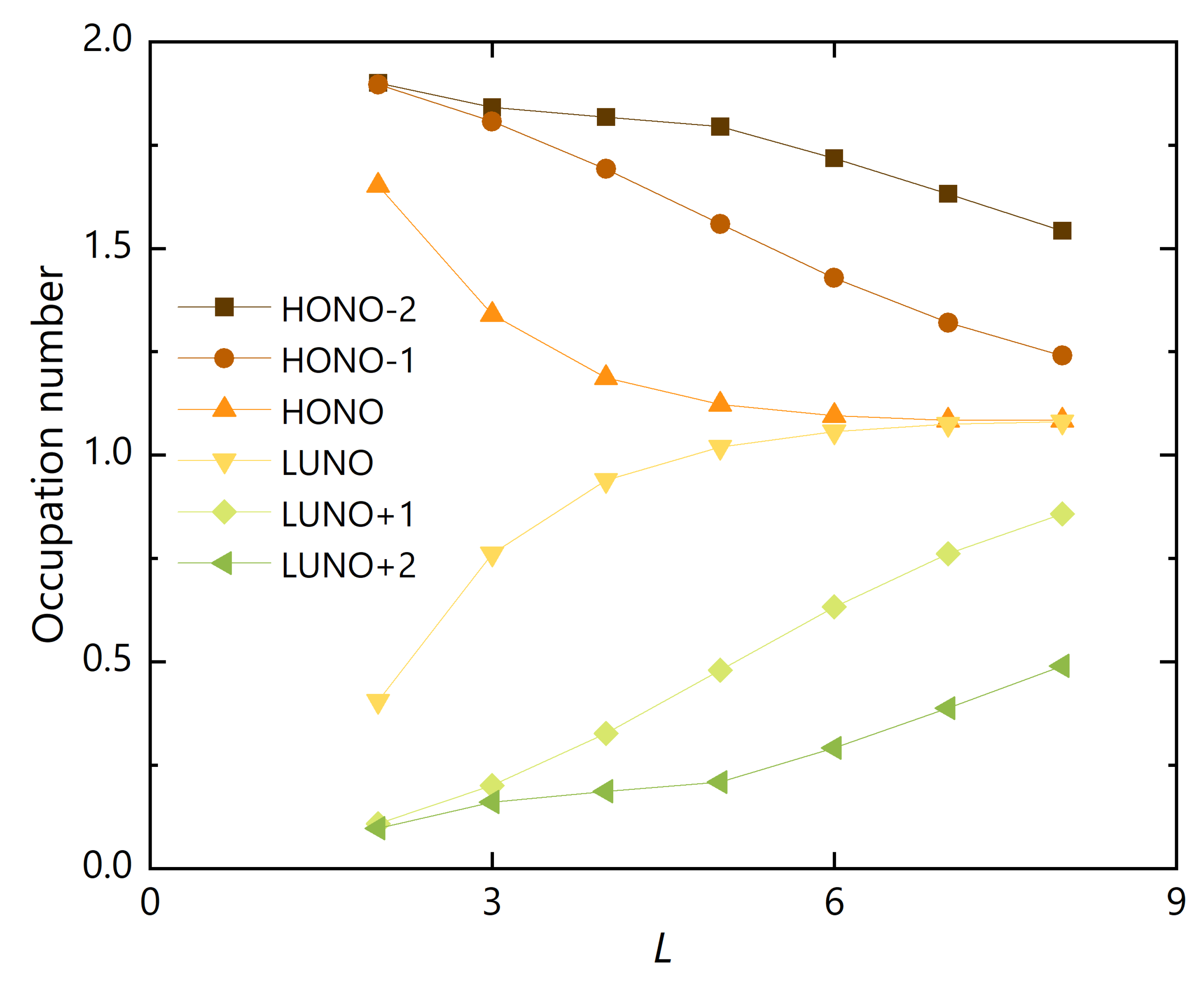
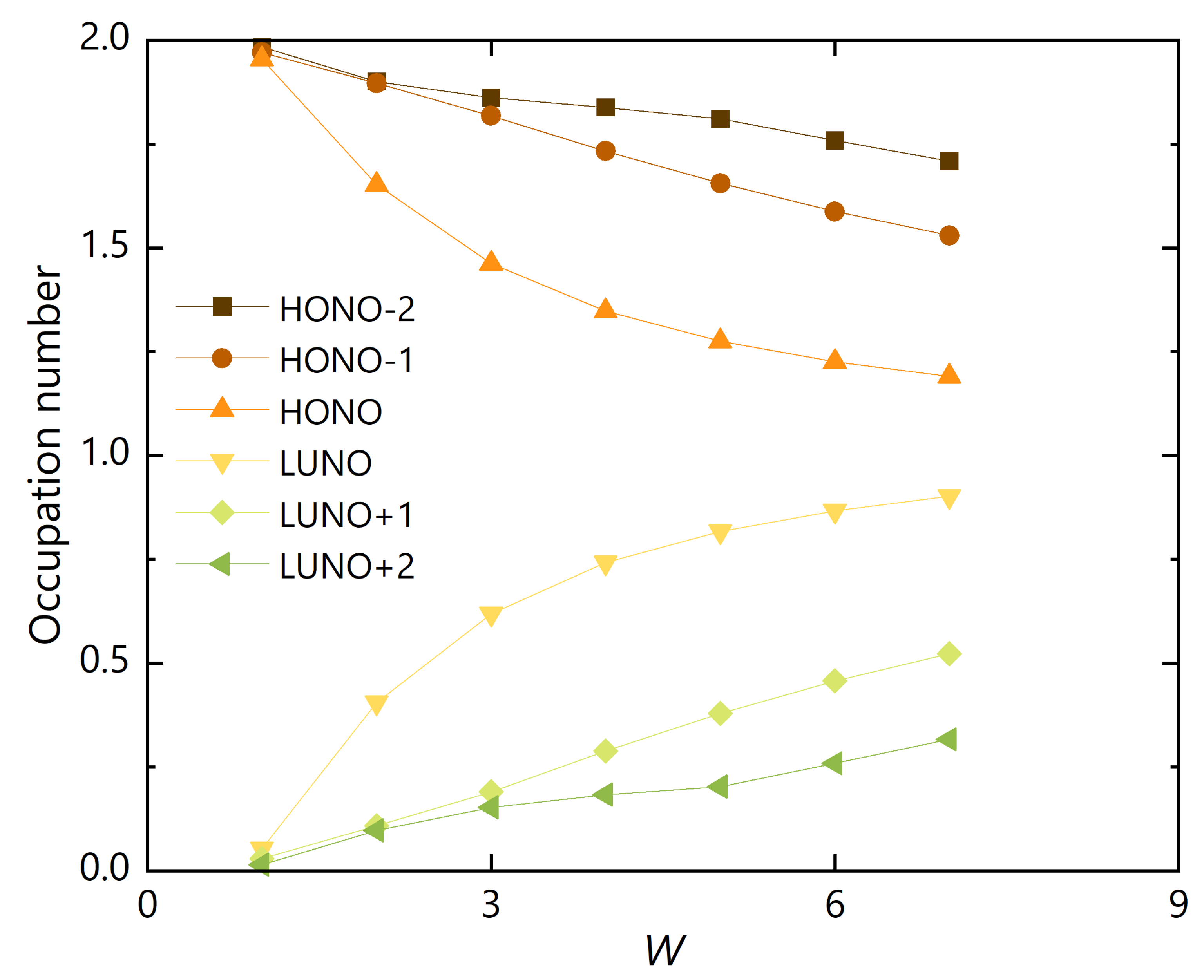
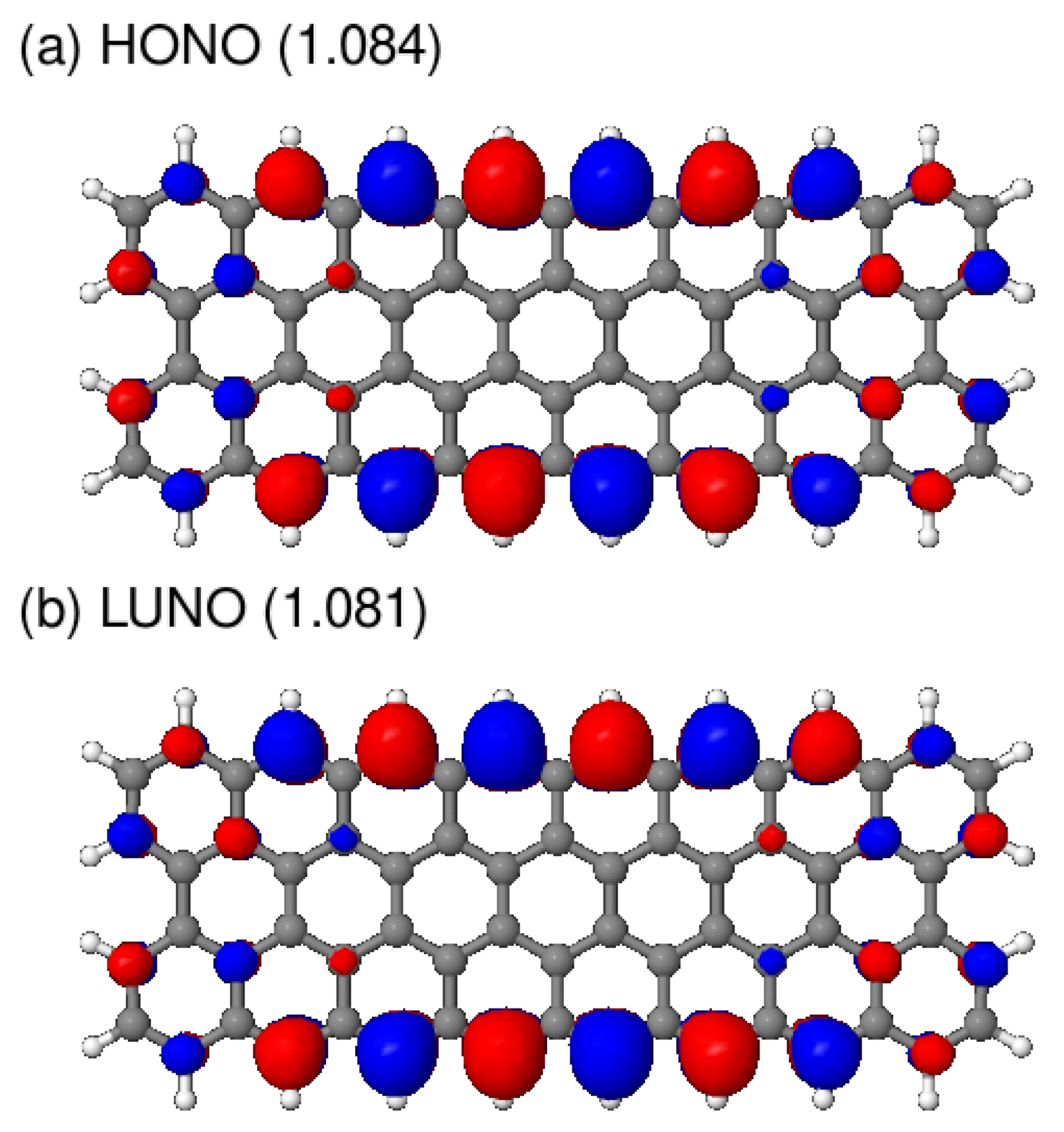
3.2. Polyradicality of Graphene Nanoribbons
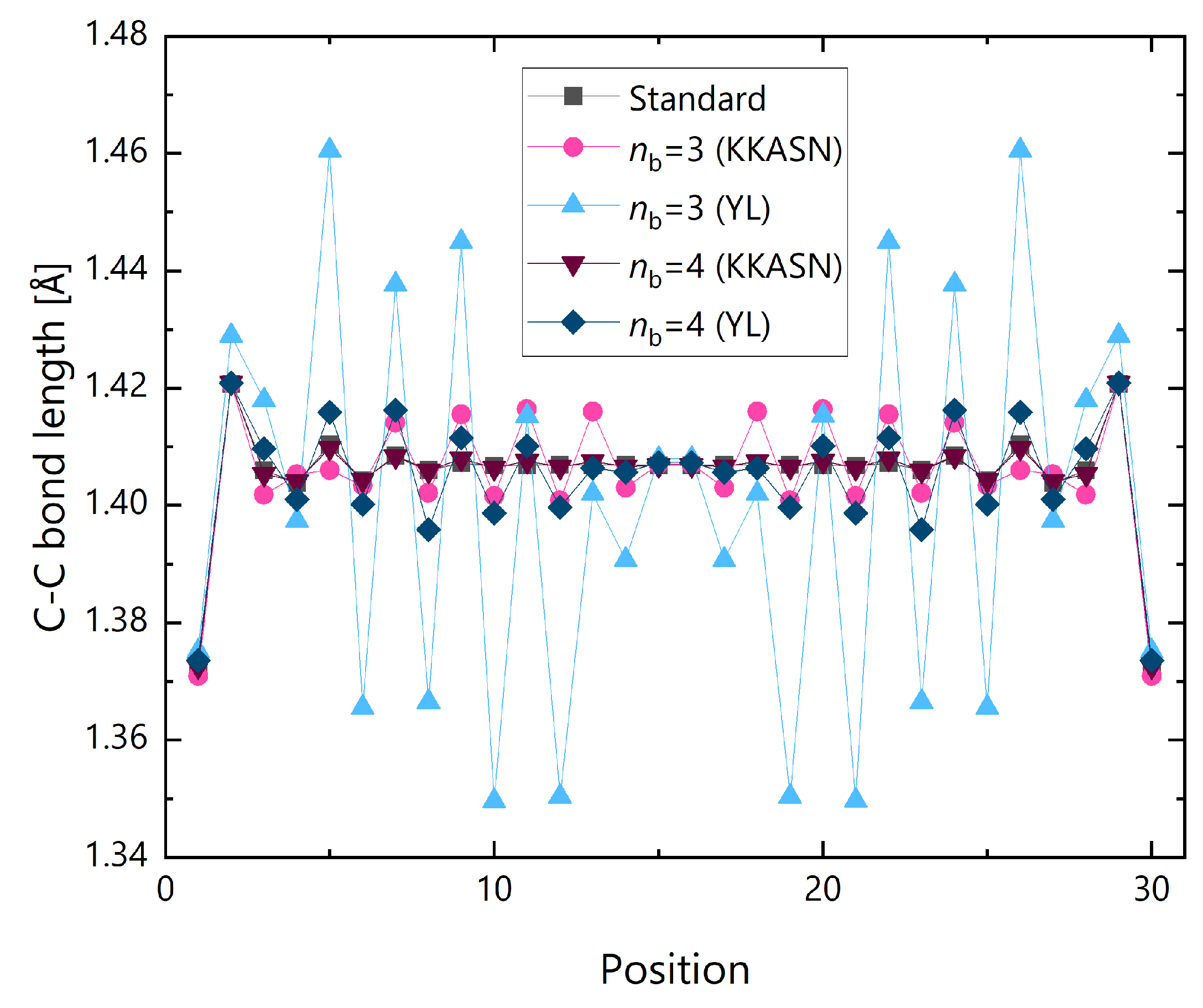
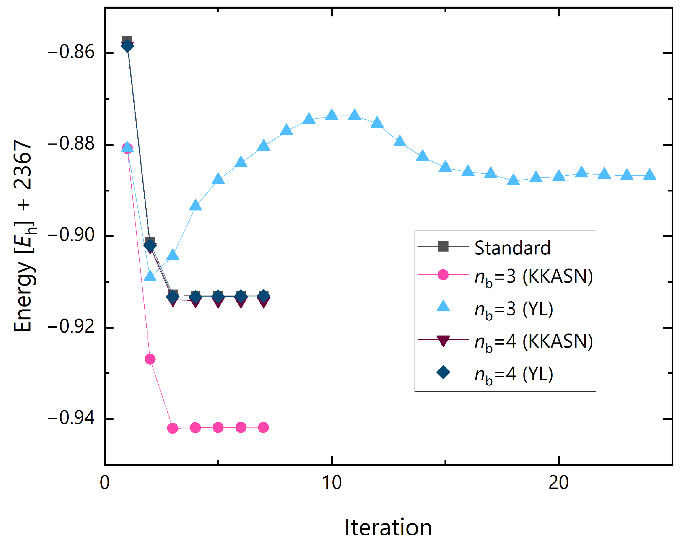
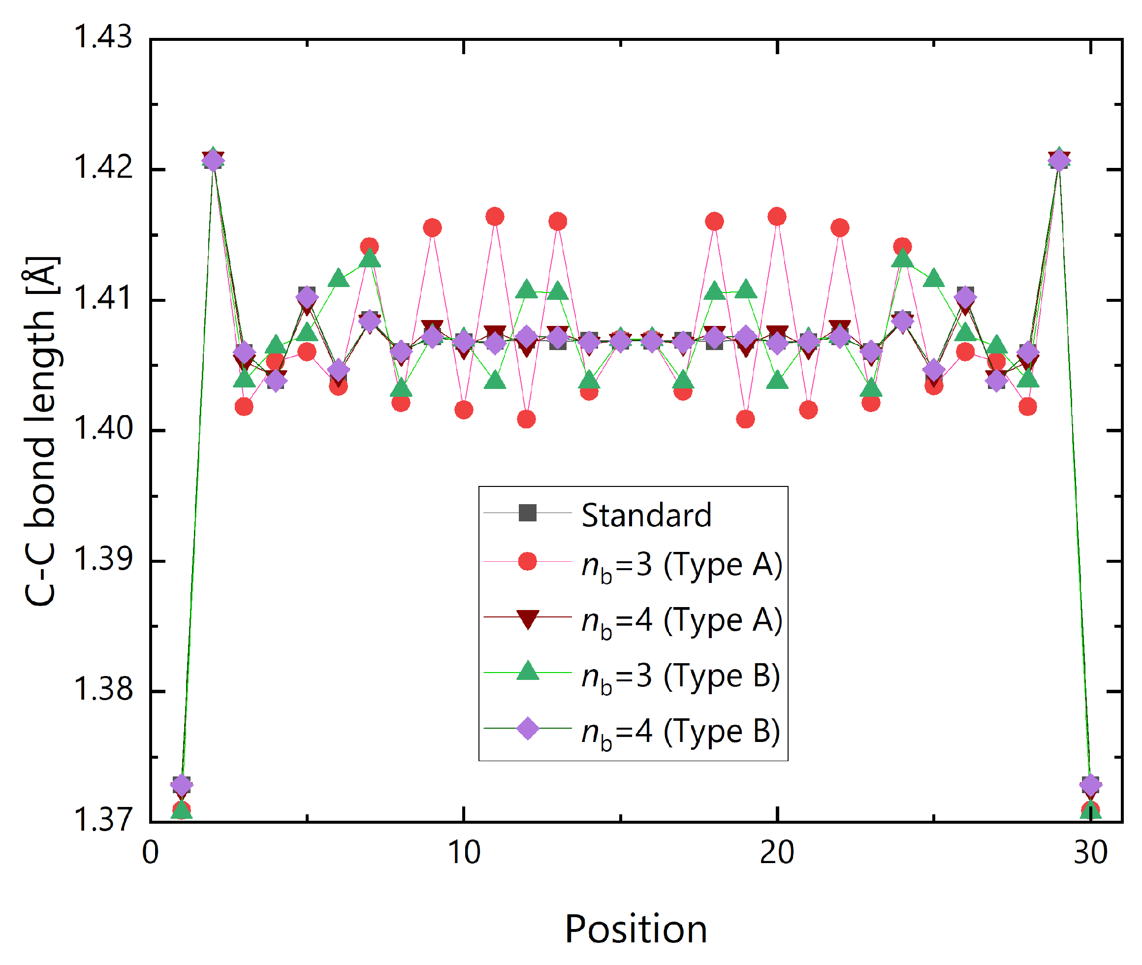
3.3. DC-HFB Optimization of GNR Structures
4. Concluding Remarks
Supplementary Materials
Author Contributions
Funding
Data Availability Statement
Acknowledgments
Conflicts of Interest
References
- Houk, K.N.; Lee, P.S.; Nendel, M. Polyacene and Cyclacene Geometries and Electronic Structures: Bond Equalization, Vanishing Band Gaps, and Triplet Ground States Contrast with Polyacetylene. J. Org. Chem. 2001, 66, 5517–5521. [Google Scholar] [CrossRef]
- Tian, C.; Miao, W.; Zhao, L.; Wang, J. Graphene nanoribbons: Current status and challenges as quasi-one-dimensional nanomaterials. Rev. Phys. 2023, 10, 100082. [Google Scholar] [CrossRef]
- Caetano, E.W.S.; Freire, V.N.; dos Santos, S.G.; Galvão, D.S.; Sato, F. Möbius and twisted graphene nanoribbons: Stability, geometry, and electronic properties. J. Chem. Phys. 2008, 128, 164719. [Google Scholar] [CrossRef]
- Mizukami, W.; Kurashige, Y.; Yanai, T. More π Electrons Make a Difference: Emergence of Many Radicals on Graphene Nanoribbons Studied by Ab Initio DMRG Theory. J. Chem. Theory Comput. 2012, 9, 401–407. [Google Scholar] [CrossRef]
- Hayes, E.F.; Siu, A.K.Q. Electronic structure of the open forms of three-membered rings. J. Am. Chem. Soc. 1971, 93, 2090–2091. [Google Scholar] [CrossRef]
- Head-Gordon, M. Characterizing unpaired electrons from the one-particle density matrix. Chem. Phys. Lett. 2003, 372, 508–511. [Google Scholar] [CrossRef]
- Nakano, M.; Fukui, H.; Minami, T.; Yoneda, K.; Shigeta, Y.; Kishi, R.; Champagne, B.; Botek, E.; Kubo, T.; Ohta, K.; et al. (Hyper)polarizability density analysis for open-shell molecular systems based on natural orbitals and occupation numbers. Theor. Chem. Accounts 2011, 130, 711–724. [Google Scholar] [CrossRef]
- Nakano, M. Excitation Energies and Properties of Open-Shell Singlet Molecules: Applications to a New Class of Molecules for Nonlinear Optics and Singlet Fission; Springer International Publishing: Cham, Switzerland, 2014. [Google Scholar] [CrossRef]
- Nakano, M. Open-Shell-Character-Based Molecular Design Principles: Applications to Nonlinear Optics and Singlet Fission. Chem. Rec. 2016, 17, 27–62. [Google Scholar] [CrossRef]
- Nakano, M.; Champagne, B. Nonlinear optical properties in open-shell molecular systems. WIREs Comput. Mol. Sci. 2016, 6, 198–210. [Google Scholar] [CrossRef]
- Roos, B.O. The Complete Active Space Self-Consistent Field Method and Its Applications in Electronic Structure Calculations; Wiley Blackwell (John Wiley & Sons): Hoboken, NJ, USA, 1987; pp. 399–445. [Google Scholar] [CrossRef]
- Zgid, D.; Nooijen, M. The density matrix renormalization group self-consistent field method: Orbital optimization with the density matrix renormalization group method in the active space. J. Chem. Phys. 2008, 128, 144116. [Google Scholar] [CrossRef]
- Nakatani, N.; Guo, S. Density matrix renormalization group (DMRG) method as a common tool for large active-space CASSCF/CASPT2 calculations. J. Chem. Phys. 2017, 146, 094102. [Google Scholar] [CrossRef]
- Olivares-Amaya, R.; Hu, W.; Nakatani, N.; Sharma, S.; Yang, J.; Chan, G.K.L. The ab-initio density matrix renormalization group in practice. J. Chem. Phys. 2015, 142, 034102. [Google Scholar] [CrossRef] [PubMed]
- Baiardi, A.; Reiher, M. The density matrix renormalization group in chemistry and molecular physics: Recent developments and new challenges. J. Chem. Phys. 2020, 152, 040903. [Google Scholar] [CrossRef] [PubMed]
- Surján, P.R. An Introduction to the Theory of Geminals. In Correlation and Localization; Topics in Current Chemistry; Surján, P.R., Ed.; Springer: Berlin/Heidelberg, Germany, 1999; Volume 203, pp. 63–88. [Google Scholar] [CrossRef]
- Limacher, P.A.; Ayers, P.W.; Johnson, P.A.; De Baerdemacker, S.; Van Neck, D.; Bultinck, P. A New Mean-Field Method Suitable for Strongly Correlated Electrons: Computationally Facile Antisymmetric Products of Nonorthogonal Geminals. J. Chem. Theory Comput. 2013, 9, 1394–1401. [Google Scholar] [CrossRef]
- Tarumi, M.; Kobayashi, M.; Nakai, H. Accelerating convergence in the antisymmetric product of strongly orthogonal geminals method. Int. J. Quantum Chem. 2013, 113, 239–244. [Google Scholar] [CrossRef]
- Bobrowicz, F.W.; Goddard, W.A. The Self-Consistent Field Equations for Generalized Valence Bond and Open-Shell Hartree—Fock Wave Functions. In Methods of Electronic Structure Theory; Springer: New York, NY, USA, 1977; pp. 79–127. [Google Scholar] [CrossRef]
- Kobayashi, M.; Szabados, Á.; Nakai, H.; Surján, P.R. Generalized Møller-Plesset Partitioning in Multiconfiguration Perturbation Theory. J. Chem. Theory Comput. 2010, 6, 2024–2033. [Google Scholar] [CrossRef]
- Tarumi, M.; Kobayashi, M.; Nakai, H. Generalized Møller-Plesset Multiconfiguration Perturbation Theory Applied to an Open-Shell Antisymmetric Product of Strongly Orthogonal Geminals Reference Wave Function. J. Chem. Theory Comput. 2012, 8, 4330–4335. [Google Scholar] [CrossRef]
- Wang, Q.; Duan, M.; Xu, E.; Zou, J.; Li, S. Describing Strong Correlation with Block-Correlated Coupled Cluster Theory. J. Phys. Chem. Lett. 2020, 11, 7536–7543. [Google Scholar] [CrossRef]
- Henderson, T.M.; Bulik, I.W.; Scuseria, G.E. Pair extended coupled cluster doubles. J. Chem. Phys. 2015, 142, 214116. [Google Scholar] [CrossRef]
- Lehtola, S.; Head-Gordon, M. Coupled-cluster pairing models for radicals with strong correlations. arXiv 2025. [Google Scholar] [CrossRef]
- Staroverov, V.N.; Scuseria, G.E. Optimization of density matrix functionals by the Hartree-Fock-Bogoliubov method. J. Chem. Phys. 2002, 117, 11107–11112. [Google Scholar] [CrossRef]
- Scuseria, G.E.; Jiménez-Hoyos, C.A.; Henderson, T.M.; Samanta, K.; Ellis, J.K. Projected quasiparticle theory for molecular electronic structure. J. Chem. Phys. 2011, 135, 124108. [Google Scholar] [CrossRef] [PubMed]
- Yang, W.; Lee, T.S. A density-matrix divide-and-conquer approach for electronic structure calculations of large molecules. J. Chem. Phys. 1995, 103, 5674–5678. [Google Scholar] [CrossRef]
- Nakai, H.; Kobayashi, M.; Yoshikawa, T.; Seino, J.; Ikabata, Y.; Nishimura, Y. Divide-and-Conquer Linear-Scaling Quantum Chemical Computations. J. Phys. Chem. A 2023, 127, 589–618. [Google Scholar] [CrossRef]
- Kobayashi, M.; Nakai, H. Divide-and-conquer approaches to quantum chemistry: Theory and implementation. In Linear-Scaling Techniques in Computational Chemistry and Physics: Methods and Applications; Challenges and Advances in Computational Chemistry and Physics; Chapter 5; Papadopoulos, M.G., Zalesny, R., Mezey, P.G., Leszczynski, J., Eds.; Springer: Dordrecht, The Netherlands, 2011; Volume 13, pp. 97–127. [Google Scholar] [CrossRef]
- Kobayashi, M.; Taketsugu, T. Divide-and-Conquer Hartree-Focko-Bogoliubov Method and Its Application to Conjugated Diradical Systems. Chem. Lett. 2016, 45, 1268–1270. [Google Scholar] [CrossRef]
- Pulay, P. Analytical derivatives, forces, force constants, molecular geometries, and related response properties in electronic structure theory. WIREs Comput. Mol. Sci. 2014, 4, 169–181. [Google Scholar] [CrossRef]
- Kobayashi, M. Gradient of molecular Hartree–Fock–Bogoliubov energy with a linear combination of atomic orbital quasiparticle wave functions. J. Chem. Phys. 2014, 140, 084115. [Google Scholar] [CrossRef]
- Chai, J.D. Density functional theory with fractional orbital occupations. J. Chem. Phys. 2012, 136, 154104. [Google Scholar] [CrossRef]
- Wu, C.S.; Chai, J.D. Electronic Properties of Zigzag Graphene Nanoribbons Studied by TAO-DFT. J. Chem. Theory Comput. 2015, 11, 2003–2011. [Google Scholar] [CrossRef]
- Chen, B.J.; Chai, J.D. TAO-DFT fictitious temperature made simple. RSC Adv. 2022, 12, 12193–12210. [Google Scholar] [CrossRef]
- Kobayashi, M.; Kunisada, T.; Akama, T.; Sakura, D.; Nakai, H. Reconsidering an analytical gradient expression within a divide-and-conquer self-consistent field approach: Exact formula and its approximate treatment. J. Chem. Phys. 2011, 134, 034105. [Google Scholar] [CrossRef] [PubMed]
- Pulay, P. Ab initio calculation of force constants and equilibrium geometries in polyatomic molecules. I. Theory. Mol. Phys. 1969, 17, 197–204. [Google Scholar] [CrossRef]
- Bolotin, K.I.; Ghahari, F.; Shulman, M.D.; Stormer, H.L.; Kim, P. Observation of the fractional quantum Hall effect in graphene. Nature 2009, 462, 196–199. [Google Scholar] [CrossRef] [PubMed]
- Novoselov, K.S.; Geim, A.K.; Morozov, S.V.; Jiang, D.; Katsnelson, M.I.; Grigorieva, I.V.; Dubonos, S.V.; Firsov, A.A. Two-dimensional gas of massless Dirac fermions in graphene. Nature 2005, 438, 197–200. [Google Scholar] [CrossRef]
- Zhang, Y.; Tan, Y.W.; Stormer, H.L.; Kim, P. Experimental observation of the quantum Hall effect and Berry’s phase in graphene. Nature 2005, 438, 201–204. [Google Scholar] [CrossRef]
- Son, Y.W.; Cohen, M.L.; Louie, S.G. Energy Gaps in Graphene Nanoribbons. Phys. Rev. Lett. 2006, 97, 216803. [Google Scholar] [CrossRef]
- Barone, V.; Hod, O.; Scuseria, G.E. Electronic Structure and Stability of Semiconducting Graphene Nanoribbons. Nano Lett. 2006, 6, 2748–2754. [Google Scholar] [CrossRef]
- Hachmann, J.; Dorando, J.J.; Avilés, M.; Chan, G.K.L. The radical character of the acenes: A density matrix renormalization group study. J. Chem. Phys. 2007, 127, 134309. [Google Scholar] [CrossRef]
- Pelzer, K.; Greenman, L.; Gidofalvi, G.; Mazziotti, D.A. Strong Correlation in Acene Sheets from the Active-Space Variational Two-Electron Reduced Density Matrix Method: Effects of Symmetry and Size. J. Phys. Chem. A 2011, 115, 5632–5640. [Google Scholar] [CrossRef]
- Pulay, P.; Hamilton, T.P. UHF natural orbitals for defining and starting MC-SCF calculations. J. Chem. Phys. 1988, 88, 4926–4933. [Google Scholar] [CrossRef]
- Schmidt, M.W.; Baldridge, K.K.; Boatz, J.A.; Elbert, S.T.; Gordon, M.S.; Jensen, J.H.; Koseki, S.; Matsunaga, N.; Nguyen, K.A.; Su, S.; et al. General atomic and molecular electronic structure system. J. Comput. Chem. 1993, 14, 1347–1363. [Google Scholar] [CrossRef]
- Gordon, M.S.; Schmidt, M.W. Advances in electronic structure theory: GAMESS a decade later. In Theory and Applications of Computational Chemistry: The First Forty Years; Chapter 41; Dykstra, C.E., Frenking, G., Kim, K.S., Scuseria, G.E., Eds.; Elsevier: Amsterdam, The Netherlands, 2005; pp. 1167–1189. [Google Scholar]
- Li Manni, G.; Galván, I.F.; Alavi, A.; Aleotti, F.; Aquilante, F.; Autschbach, J.; Avagliano, D.; Baiardi, A.; Bao, J.J.; Battaglia, S.; et al. The OpenMolcas Web: A Community-Driven Approach to Advancing Computational Chemistry. J. Chem. Theory Comput. 2023, 19, 6933–6991. [Google Scholar] [CrossRef] [PubMed]
- Hehre, W.J.; Ditchfield, R.; Pople, J.A. Self-consistent molecular orbital methods. XII. Further extensions of Gaussian-type basis sets for use in molecular orbital studies of organic molecules. J. Chem. Phys. 1972, 56, 2257. [Google Scholar] [CrossRef]
- Hariharan, P.C.; Pople, J.A. The influence of polarization functions on molecular orbital hydrogenation energies. Theor. Chim. Acta 1973, 28, 213–222. [Google Scholar] [CrossRef]
- Tsuchimochi, T.; Scuseria, G.E.; Savin, A. Constrained-pairing mean-field theory. III. Inclusion of density functional exchange and correlation effects via alternative densities. J. Chem. Phys. 2010, 132, 024111. [Google Scholar] [CrossRef]
- Nishida, M.; Akama, T.; Kobayashi, M.; Taketsugu, T. Time-dependent Hartree–Fock–Bogoliubov method for molecular systems: An alternative excited-state methodology including static electron correlation. Chem. Phys. Lett. 2023, 816, 140386. [Google Scholar] [CrossRef]
- Jiménez-Hoyos, C.A.; Henderson, T.M.; Tsuchimochi, T.; Scuseria, G.E. Projected Hartree–Fock theory. J. Chem. Phys. 2012, 136, 164109. [Google Scholar] [CrossRef]


| HFB | |||||||
|---|---|---|---|---|---|---|---|
| Molecule | Position | CASSCF | ζ = 0.75 | 0.80 | 0.85 | 0.90 | 1.00 |
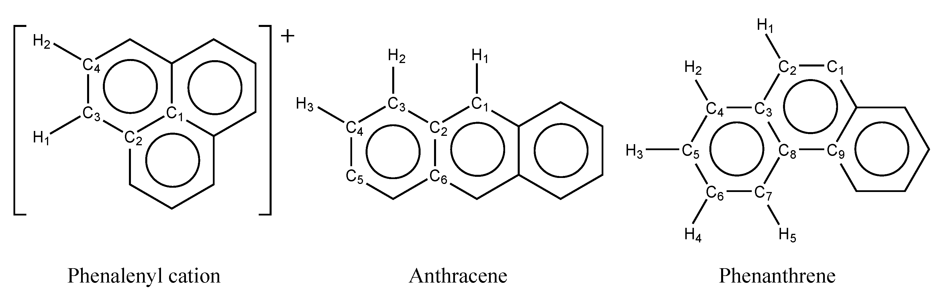
| Phenalenyl cation | C1–C2 | 1.4178 | 1.4107 | 1.4164 | 1.4228 | 1.4297 | 1.4487 |
| C2–C3 | 1.4141 | 1.4087 | 1.4121 | 1.4157 | 1.4198 | 1.4344 | |
| C3–C4 | 1.3921 | 1.3834 | 1.3873 | 1.3921 | 1.3982 | 1.4173 | |
| Anthracene | C1–C2 | 1.4008 | 1.3894 | 1.3893 | 1.4009 | 1.4106 | 1.4299 |
| C2–C3 | 1.4385 | 1.4359 | 1.4359 | 1.4252 | 1.4218 | 1.4343 | |
| C3–C4 | 1.3649 | 1.3473 | 1.3473 | 1.3671 | 1.3863 | 1.4156 | |
| C4–C5 | 1.4337 | 1.4324 | 1.4325 | 1.4183 | 1.4114 | 1.4213 | |
| C2–C6 | 1.4287 | 1.4246 | 1.4245 | 1.4330 | 1.4409 | 1.4557 | |
| Phenanthrene | C1–C2 | 1.3557 | 1.3386 | 1.3386 | 1.3479 | 1.3730 | 1.4080 |
| C2–C3 | 1.4424 | 1.4405 | 1.4405 | 1.4356 | 1.4269 | 1.4329 | |
| C3–C4 | 1.4166 | 1.4084 | 1.4084 | 1.4100 | 1.4163 | 1.4341 | |
| C4–C5 | 1.3780 | 1.3656 | 1.3656 | 1.3707 | 1.3856 | 1.4134 | |
| C5–C6 | 1.4090 | 1.4017 | 1.4017 | 1.4022 | 1.4048 | 1.4188 | |
| C6–C7 | 1.3802 | 1.3677 | 1.3677 | 1.3730 | 1.3886 | 1.4165 | |
| C3–C8 | 1.4127 | 1.4043 | 1.4043 | 1.4127 | 1.4324 | 1.4570 | |
| C7–C8 | 1.4192 | 1.4106 | 1.4106 | 1.4119 | 1.4177 | 1.4370 | |
| C8–C9 | 1.4634 | 1.4612 | 1.4612 | 1.4576 | 1.4520 | 1.4589 | |
| MAD | 0.0080 | 0.0073 | 0.0057 | 0.0113 | 0.0251 | ||
| HFB | |||||||
|---|---|---|---|---|---|---|---|
| Molecule | Position | CASSCF | ζ = 0.75 | 0.80 | 0.85 | 0.90 | 1.00 |
| Phenalenyl cation | C3–H1 | 1.0752 | 1.0758 | 1.0753 | 1.0752 | 1.0755 | 1.0791 |
| C4–H2 | 1.0734 | 1.0731 | 1.0736 | 1.0741 | 1.0747 | 1.0784 | |
| Anthracene | C1–H1 | 1.0769 | 1.0768 | 1.0768 | 1.0768 | 1.0773 | 1.0818 |
| C3–H2 | 1.0763 | 1.0762 | 1.0762 | 1.0763 | 1.0767 | 1.0806 | |
| C4–H3 | 1.0756 | 1.0756 | 1.0756 | 1.0757 | 1.0760 | 1.0796 | |
| Phenanthrene | C2–H1 | 1.0761 | 1.0761 | 1.0761 | 1.0761 | 1.0765 | 1.0806 |
| C4–H2 | 1.0763 | 1.0763 | 1.0763 | 1.0763 | 1.0767 | 1.0806 | |
| C5–H3 | 1.0755 | 1.0755 | 1.0755 | 1.0755 | 1.0759 | 1.0794 | |
| C6–H4 | 1.0756 | 1.0757 | 1.0757 | 1.0757 | 1.0760 | 1.0797 | |
| C7–H5 | 1.0727 | 1.0727 | 1.0727 | 1.0728 | 1.0732 | 1.0776 | |
| MAD | 0.0001 | 0.0001 | 0.0001 | 0.0005 | 0.0044 | ||
| Method | Time |
|---|---|
| Standard UHF | 232.1 |
| Standrad HFB () | 3765.5 |
| DC-HFB () | 1396.0 |
Disclaimer/Publisher’s Note: The statements, opinions and data contained in all publications are solely those of the individual author(s) and contributor(s) and not of MDPI and/or the editor(s). MDPI and/or the editor(s) disclaim responsibility for any injury to people or property resulting from any ideas, methods, instructions or products referred to in the content. |
© 2025 by the authors. Licensee MDPI, Basel, Switzerland. This article is an open access article distributed under the terms and conditions of the Creative Commons Attribution (CC BY) license (https://creativecommons.org/licenses/by/4.0/).
Share and Cite
Kobayashi, M.; Kodama, R.; Akama, T.; Taketsugu, T. Fragmentation-Based Linear-Scaling Method for Strongly Correlated Systems: Divide-and-Conquer Hartree–Fock–Bogoliubov Method, Its Energy Gradient, and Applications to Graphene Nano-Ribbon Systems. Chemistry 2025, 7, 46. https://doi.org/10.3390/chemistry7020046
Kobayashi M, Kodama R, Akama T, Taketsugu T. Fragmentation-Based Linear-Scaling Method for Strongly Correlated Systems: Divide-and-Conquer Hartree–Fock–Bogoliubov Method, Its Energy Gradient, and Applications to Graphene Nano-Ribbon Systems. Chemistry. 2025; 7(2):46. https://doi.org/10.3390/chemistry7020046
Chicago/Turabian StyleKobayashi, Masato, Ryosuke Kodama, Tomoko Akama, and Tetsuya Taketsugu. 2025. "Fragmentation-Based Linear-Scaling Method for Strongly Correlated Systems: Divide-and-Conquer Hartree–Fock–Bogoliubov Method, Its Energy Gradient, and Applications to Graphene Nano-Ribbon Systems" Chemistry 7, no. 2: 46. https://doi.org/10.3390/chemistry7020046
APA StyleKobayashi, M., Kodama, R., Akama, T., & Taketsugu, T. (2025). Fragmentation-Based Linear-Scaling Method for Strongly Correlated Systems: Divide-and-Conquer Hartree–Fock–Bogoliubov Method, Its Energy Gradient, and Applications to Graphene Nano-Ribbon Systems. Chemistry, 7(2), 46. https://doi.org/10.3390/chemistry7020046