Article

Electromagnetic Signatures of Possible Charge Anomalies in Tunneling

by
Fernando Minotti
1,2 and
Giovanni Modanese
3,*
1
Departamento de Física, Facultad de Ciencias Exactas y Naturales, Universidad de Buenos Aires, Buenos Aires C1428EGA, Argentina
2
Instituto de Física del Plasma (INFIP), CONICET—Universidad de Buenos Aires, Buenos Aires C1428EGA, Argentina
3
Faculty of Science and Technology, Free University of Bozen-Bolzano, I-39100 Bolzano, Italy
*
Author to whom correspondence should be addressed.
Quantum Rep. 2022, 4(3), 277-295; https://doi.org/10.3390/quantum4030020
Submission received: 9 June 2022 / Revised: 2 August 2022 / Accepted: 4 August 2022 / Published: 11 August 2022

Abstract

:
We reconsider some well-known tunneling processes from the point of view of Aharonov-Bohm electrodynamics, a unique extension of Maxwell’s theory which admits charge-current sources that are not locally conserved. In particular we are interested into tunneling phenomena having relatively long range (otherwise the non-Maxwellian effects become irrelevant, especially at high frequency) and involving macroscopic wavefunctions and coherent matter, for which it makes sense to evaluate the classical e.m. field generated by the tunneling particles. For some condensed-matter systems, admitting discontinuities in the probability current is a possible way of formulating phenomenological models. In such cases, the Aharonov-Bohm theory offers a logically consistent approach and allows to derive observable consequences. Typical e.m. signatures of the failure of local conservation are at high frequency the generation of a longitudinal electric radiation field, and at low frequency a small effect of “missing” magnetic field. Possible causes of this failure are instant tunneling and phase slips in superconductors. For macroscopic quantum systems in which the phase-number uncertainty relation Δ N Δ φ 1 applies, the expectation value of the anomalous source I = t ρ + · j has quantum fluctuations, thus becoming a random source of weak non-Maxwellian fields.

1. Introduction

The tunneling effect is one of the most typical features of quantum mechanics, and a clear demonstration of the wavelike behavior of matter at a microscopic scale (at least in the context of the standard Copenhagen interpretation). Historically, it was first observed in the decay of nuclei [1] and in field-effect emission of electrons from metals [2]. Later it was exploited, among many other applications, in Zener diodes [3,4] and in scanning tunneling microscopes [5]. Tunneling processes involving macroscopic wavefunctions in superconductors give rise to the Josephson effect [6], which has been applied to SQUIDs (super quantum interference devices), frequency standards, quantum circuits and q-bits. Long-range tunneling has an important role in chemistry and biology [7].
When the tunneling effect involves single particles or multiple incoherent particles, it can be usually described by theoretical models based on a Schrödinger equation and its exact or approximate solutions. We thus have a theory in which the wavefunction in the barrier is known and we can evaluate in principle the probability for the tunneling particles to be located at any position in the classically forbidden region. At the same time, we can compute the probability density ρ = | Ψ | 2 and the probability current j = ( i e / 2 m ) ( Ψ * Ψ Ψ Ψ * ) , which satisfy the continuity relation t ρ + · j = 0 thanks to a general property of the solutions of the Schrödinger equation.
By inserting the source ( ρ , j ) into the Maxwell equations we can then compute in principle the e.m. field generated by the tunneling current. In most cases this field is not detectable, because the number of tunneling particles is small, and their current too. Actually, for tunneling processes at the atomic level, e.m. emissions are more properly evaluated with quantum perturbation theory than by solving Maxwell equations.
On the other hand, when the tunneling involves a large number of particles, it cannot be described by a simple Schrödinger equation. This is the case of tunneling in condensed matter, be it incoherent or coherent (for coherent matter with a macroscopic wavefunction there are some further specifications, see below). In this case we do not know the wavefunction in the barrier and we usually cannot locate the particles in the barrier with a definite probability as a function of space and time; we only know a tunneling probability, or more generally a tunneling Hamiltonian operator that can be applied between initial and final states on the two sides of the barrier.
For condensed matter systems it is generally possible to define a quantum field theory with local interactions, which includes charge and current operators satisfying a local conservation relation analogous to t ρ + · j = 0 . The next step, however, is often to introduce approximations and effective models with non-local interactions. Furthermore, even in the original local theory, quantum anomalies may occur after renormalization, spoiling the symmetry and conservation properties of the original Hamiltonian [8,9,10]. In most approaches to quantum transport there is no attempt to compute the wavefunction of tunneling particles in the barrier. The issue of tunneling time has been lively debated, and it is both based on experimental results and theoretical models; according to some authors, in certain cases the tunneling time cannot be distinguished from zero [11,12,13].
A recent series of sophisticated numerical first-principles calculations of the local current density in organic molecular chains and carbon wires [14,15,16,17] confirm the existence of discontinuities in the stationary local flux, which are not eliminated by an enlargement of the wavefunctions eigenbasis employed. Already in 2008, Wang et al. [18] had shown that in such cases the Landauer-Büttiker formalism leads to restore conservation by the introduction of a non-local secondary current of the form j n = χ , where 2 χ = I , with our notation, in the stationary case. The applications treated by Wang et al. concerned some idealized materials and graphene [19], while Gardner et al. [16,17] compute explicitly the part of the flux that does not follow molecular bonds for specific saturated molecules.
Nozaki et al. [20] point out that a precise knowledge of magnetic field patterns in molecular devices can be important for applications to molecular magnets. This leads us to ask a logical theoretical question (but also with possible practical implications): how should one compute the e.m. field of a microscopic current that is not locally conserved? A first answer can be, that since the non-local extension of the current proposed by Wang restores conservation, the Maxwell equations can be applied to such a “completed” current.
A more complete and powerful approach, however, consists of extending Maxwell’s theory along the lines originally proposed by Aharonov and Bohm [21] and by Ohmura [22]. This theory allows us to compute e.m. fields, compatibly with Special Relativity, even when charge is not locally conserved, avoiding the need to impose a “taboo on teleportation”, at least in phenomenological models. It also applies to generalized microscopic models with fractional dimensions and non-local potentials. There has been much work on this extended theory over the last years, and many technical aspects have been clarified [21,23,24,25,26,27,28,29]. The final recipe is unique and relatively simple, considering that some non-local expressions involving the sources are unavoidable. In Section 2 of this work we recall the extended equations for the e.m. fields and their far-field solution in the oscillating dipole approximation. We also recall the relations concerning the extended Lorenz force and energy-momentum conservation.
In Section 3 we introduce a simple model for discontinuous microscopic currents in a metal. We show that the effective/averaged consequence of the microscopic discontinuities is to generate an extra-source whose moment δ P is proportional to the average macroscopic density J : δ P = γ J δ V . The coefficient γ is in turn proportional to the number of discontinuities per unit volume, to their average length and average current affected. This method is applied to a resonating cavity with a mode TM 0 10 and allows to compute the anomalous longitudinal electric field E L in the far-field region along the axis of the cavity.
In Section 4 we introduce a 1-D model for resonant tunneling in a metal based on the Kronig-Penney 1-D model of a crystal lattice consisting in square potential barriers. This simple model can be solved exactly and allows to interpret at least part of the conduction current as due to long-range resonant tunneling of valence electrons, with transmission coefficient T = 1 .
Section 5 and Section 6 are devoted to macroscopic quantum systems described by a collective wavefunction. In Section 5 we consider the effect of quantum fluctuations in a Josephson junction oscillating at its plasma frequency. Due to the uncertainty on the product Δ φ Δ N , the expectation value of the anomaly I cannot be exactly zero and in a semiclassical approximation this generates in general a random longitudinal electric field in the radiation region.
In Section 6 we consider solutions of the Ginzburg-Landau equation describing a superconducting weak link and we check the claim, often found in the literature, that such solutions can contain points at which ψ = 0 and the quantum phase can “slip” freely. We conclude that this is not possible if the local conservation of charge holds exactly.

2. Extended Field Equations and Energy-Momentum Relations

In the Aharonov-Bohm theory of extended electrodynamics the gauge invariance of the four-potentials is reduced to transformations of the form A μ A μ + μ χ , where χ = 0 . (Here we define A μ = ( ϕ / c , A ) , being ϕ the electric potential and A the vector potential. The metric has signature ( + , , , ) , with coordinates x μ = ( x 0 , x 1 , x 2 , x 3 ) and x 0 = c t .)
The four-divergence of A μ is promoted to a dynamical field S ( S = μ A μ ), obeying the equation
S = μ 0 I
where
I ( x , t ) = t ρ ( x , t ) + · j ( x , t )
often called “extra-current” or “extra-source”, is zero in standard classical situations where charge is locally conserved but can be different from zero in more general settings, for example in fractional quantum mechanics or in the presence of non-local potentials in the Schrödinger equation.
The extended first and fourth Maxwell equations are in SI units
· E = ρ ε 0 S t
× B = μ 0 j + ε 0 μ 0 E t + S
where one recognizes additional sources ε 0 S / t and μ 0 S which, due to Equation (1), can be spread out in space, far away from the physical sources ρ and j .
The second and third Maxwell equations remain valid in their familiar form, and also the wave equations for E and B retain their usual form
E = μ 0 j t + c 2 ρ
B = μ 0 × j
Nevertheless, due to the appearance of S in Equations (3) and (4) the wave solutions of (5) and (6) can contain a longitudinal electric field which for a spherical wave in the dipole approximation has the expression  
E L = μ 0 4 π r P ˙ t r c · r r
being P is the dipole moment of the extra-current I:
P ( t ) = d 3 x x I ( x , t )
If we apply Equation (6) to a stationary current with some interruptions (due to “instant tunneling” or other failures of local conservation of charge), the Biot-Savart law predicts an effect of “missing B ” from the regions with j = 0 ; the prediction is confirmed by full integration of (6). An experiment proposed for the detection of this effect is described in [30], while in Section 3 of this work we discuss the case of high-frequency currents circulating in the walls of a resonant cavity.
A complex calculation [31] shows that the energy-momentum tensor of the e.m. field in Aharonov-Bohm theory is given by the usual Maxwell tensor T μ ν M plus a term depending on S:
T μ ν A B = T μ ν M + T μ ν S
T μ ν M = 1 μ 0 F μ ρ F ν ρ 1 4 F ρ σ F ρ σ η μ ν
T μ ν S = 1 μ 0 A μ ν S + A ν μ S 1 2 S 2 + A ρ ρ S η μ ν
By imposing the conservation of the total energy-momentum of field and matter, namely
μ T μ ν A B + T μ ν m a t t e r = 0
one obtains equations for the power w exerted by the field on matter, and for the force f per unit volume on matter (extended Lorenz force):
w = j · E I ϕ ,
f = ρ E + j × B I A .
We thus see that the potentials have a direct effect on matter where I 0 . Since gauge invariance is strongly reduced, under suitable boundary conditions at infinity for the potentials, w and f can be in principle computed without any ambiguities.

3. A Simple Model for Discontinuous Currents in a Conductor

In this section we give a first example of a possible application of the Aharonov-Bohm extended electrodynamics in a phenomenological model of condensed matter physics.
We start with the assumption that when current circulates in a conductor part of it is due to resonant tunneling of bound electrons close to the Fermi level, and that this tunneling can be interpreted as a discontinuous transport of those electrons across the classically forbidden zones.
If there is an electron current of value i n that discontinuously crosses from the point x n to the point x n + d n , the corresponding extra source is
I n = i n δ x x n d n δ x x n .
This can be easily seen if one considers the integral over an arbitrary volume V
V I d V = V ρ t + · j d V = S V j D · d S ,
where j D represents the discontinuous component of the current density. By choosing V to include either x n , or  x n + d n , expression (15) is then established.
In this way, if one considers a small volume δ V , in which a number of these extra sources exist, the corresponding moment is
δ P = δ V n δ V I n x d 3 x = n δ V i n d n .
Following the previous ideas, we consider that the i n ’s amount to a fraction of the current circulating in δ V , that is j · δ S , while the d n ’s amount to a fraction of the distance δ L traversed by the current j in δ V . Since δ V = δ S δ L , a simple model reflecting these ideas is given by
δ P = n δ V i n d n = γ δ V j d 3 x = γ J δ V .
In this expression γ < 1 models the fractions previously considered, and J is the macroscopic current in the material.
Considering that it is expected that γ 1 , one can determine J using Maxwell equations, and then evaluate the anomalous effects due to the dipolar moments of the extra sources by adding up the effect of each elementary dipole, given by [31]
δ S x , t = μ 0 4 π c x x 2 t δ P x , t · x x , E L x , t = μ 0 4 π x x t δ P x , t ,
with t = t x x / c . We have in this way
S x , t = μ 0 γ 4 π c J x , t / t x x 2 · x x d 3 x ,
E L x , t = μ 0 γ 4 π J x , t / t x x d 3 x .
For the expressions of the Fourier transforms in time we have
S x , ω = i ω μ 0 γ 4 π c J x , ω x x 2 · x x e i ω c x x d 3 x , E L x , ω = i ω μ 0 γ 4 π J x , ω x x e i ω c x x d 3 x .
As an important case, let us consider the anomalous effects predicted by this model in the case of resonant EM cavities. Once the EM fields in the cavity had been determined from Maxwell equations, the current circulating in the cavity walls are determined from the condition
K = n × B μ 0 ,
evaluated at the wall, with  n the (external) unit vector normal to the wall surface considered. In this expression K is the surface current density, so that, correspondingly, in expressions (19) one makes the replacement
J x , ω d 3 x K x , ω d S ,
and extends the integral to the internal surface of the cavity.
As a relatively simple example let us consider the E L generated by the TM 010 mode of a cylindrical cavity of radius a and height d. The corresponding frequency is ω = 2.405 c / a , and the magnetic field, in cylindrical coordinates (r, φ , z), is given in terms of the Bessel function of the first kind as
B x , ω = i E 0 c J 1 2.405 r a e i ω t e φ ,
where E 0 is the electric field on the axis of the cavity.
The expression of E L is then given by
E L x , ω = ω E 0 γ a 4 π c J 1 2.405 0 d d z 0 2 π d φ e i ω c x x x x e z ,
with
x x = r 2 + z z 2 + a 2 2 a r cos φ .
In particular, along the z axis
E L r = 0 , z , ω = ω E 0 γ a 2 c J 1 2.405 0 d d z e i ω c z z 2 + a 2 z z 2 + a 2 e z ,
that for z a , d can be approximated by
E L r = 0 , z , ω i E 0 γ a 2 z 1 e i ω c d J 1 2.405 e i ω c z e z .
The advantage of considering a closed cavity is that usual transverse electromagnetic radiation is confined to the inside of the cavity. On the other hand, the longitudinal component, that according to the proposed model would be generated inside the cavity walls, is transmitted without decay inside the conductor (see Appendix A in [28]), so that it could in principle be detected outside the cavity, and its characteristics, as predicted by Equation (26), tested. For instance the z 1 decay, the  1 c o s ω c d dependence of the intensity, etc. Additionally, if a high-Q cavity is employed, intense values of E 0 can be obtained, so as to facilitate detection of E L for small values of γ .

4. Kronig-Penney 1-D Model and Resonant Tunneling

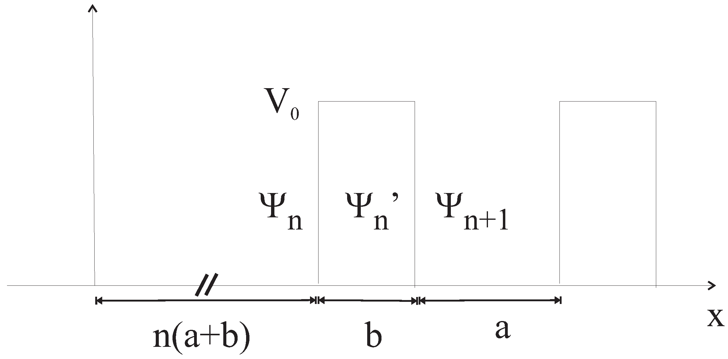
In order to qualitatively justify the assumption of long range tunneling in a metal, we consider the Kronig-Penney 1-D model of a crystal lattice consisting in square barriers of height V 0 , width b and separation a as shown in Figure 1. This potential is not meant to represent that of the bare ion lattice, but the effective, Hartree-Fock potential valid for the electrons in the highest energy levels, that includes the screening of the ion lattice potential by the lowest energy electrons.
Given the barrier at x = n a + b , the wavefunction at its left, corresponding to the energy E, is
ψ n x = A n e i k x + B n e i k x ,
the one inside the barrier
ψ n x = A n e i q x + B n e i q x ,
and that at its immediate right is
ψ n + 1 x = A n + 1 e i k x + B n + 1 e i k x ,
where,
k = 2 m E , q = 2 m E V 0 = k 1 β k a 2 ,
with
β = 2 m V 0 a 2 2 .
The boundary conditions at each side of the barrier are
ψ n x ψ n x x = n a + b = 0 ,
d ψ n d x d ψ n d x x = n a + b = 0 ,
ψ n + 1 x ψ n x x = n a + b + b = 0 ,
d ψ n + 1 d x d ψ n d x x = n a + b + b = 0 .
Solving these boundary conditions for A n + 1 and B n + 1 in terms of A n and B n results in
A n + 1 B n + 1 = M n A n B n ,
with a matrix M n whose explicit expression can be readily computed. Considering now Bloch theorem:
ψ x + a + b = ψ x e i p a + b ,
with p the quasi-momentum, one has for a generic barrier at x = n a + b that the wavefunctions at its left and right must be related by
ψ n + 1 x = ψ n x a b e i p a + b ,
that, together with the general relation (28) results in a linear, homogeneous system of equations for the coefficients A n , A n + 1 , B n , and  B n + 1 , the zero of whose determinant determines the allowed values, or bands, of k, and the value of p corresponding to each allowed k.
Alternatively, one can study the related problem of the transmission across a finite number of barriers. For this, one considers that for x < 0 there is an “incident” wave given by
ψ 0 x = A 0 e i k x + B 0 e i k x ,
while for x > N 1 a + b + b (after N barriers) there is an “emerging” wave
ψ N x = C N e i k x + D N e i k x .
Using the relations (28) we can write
C N D N = M A 0 B 0 ,
with ( M 0 at the farthest right)
M = n = N 1 n = 0 M n .
In this way, to obtain the reflection (R) and transmission (T) coefficients across the N barriers, we put A 0 = 1 , B 0 = r , C N = t , D N = 0 , to have
r = M 21 M 22 , t = M 11 M 12 M 21 M 22 ,
and
R = r , T = t ,
so that one has a resonant tunneling with perfect transmission across the N barriers when R = 0 .
As one can reasonably expect, the energy levels with zero transmission ( R = 1 ), are found inside the forbidden bands as determined by Bloch theorem. However, the relevant point is that when solving the condition for perfect transmission across N barriers one obtains N 1 solutions distributed all across each allowed band. This means that bound electrons ( E < V 0 ) with the appropriate energy could in principle tunnel freely across a large number of barriers. Of course, the exclusion principle forbids this unless there is an available state with the same energy to tunnel to.
Moreover, in a metal the conduction electrons belong in general to an allowed band that includes energy levels with E < V 0 and E > V 0 , that fill the levels up to the Fermi energy E F . A sketch of the obtained solution for five barriers is shown in Figure 2, in which the Fermi level, allowed bands and energy levels with perfect transmission across the whole lattice are shown.
Since the conduction band is not completely filled, a small energy perturbation, as produced by an applied electric field, can promote electrons with energy close to E F to higher levels. The assumption is that this effect can work on a small number of electrons in bound energy levels (close to E F ) so as to free levels for other bound electrons to resonantly tunnel to, resulting in a fraction of the electric current to be due to electrons that tunnel across a considerable distance.

5. Josephson Junctions as Random Sources of a Longitudinal Electric Field

In our work [31] we have shown that in macroscopic quantum systems for which the phase-number uncertainty relation Δ N Δ φ 1 holds, one can derive from it an uncertainty relation between charge and current in a given state:
Δ j x j x Δ ρ ρ 1 N
We have proven this formula for a Josephson junction, re-obtaining the same relation given by Devoret [32,33] and by Chen et al. [34] for Josephson junctions and more generally for quantum circuits. Then we have applied it to the quantity I = t ρ + · j = t ρ + x j x (in 1D) that we call “anomaly” because classically it is always zero. (I is also called “extra-current” in the jargon of extended electrodynamics and fractional quantum mechanics.) Focusing on a simple 1D case with time dependence ρ e i ω t and a dependence of j x on space as j x e i k x , we have written the operator I ^ as a linear combination of the operators ρ ^ and j x ^ . Considering that these operators do not have common eigenstates and satisfy (29), we have derived an estimate of the uncertainty Δ I .
The conclusion is that I ^ Ψ displays quantum fluctuations for any state Ψ and the classical conservation relation I = 0 cannot be exactly satisfied everywhere at the quantum level. We have evaluated the magnitude order of the fluctuations for the case of a specific Josephson junction operating at a resonant frequency ω 42 GHz with a current of the order of 10 4 A [35]. It turns out that Δ I 10 16 A/m 3 .
The high frequency emission of Josephson junctions is well known; usually the emitted power does not exceed a few μ W, but there have been several attempts to improve it by building arrays of synchronized junctions [36,37]. Now we hypothesize that besides the standard emission of the oscillating super-current, an anomalous emission described by extended electrodynamics could be present, namely we regard Ω ( x , t ) = I ^ Ψ as the stochastic source of a field S which is itself stochastic and can have a role in the extended Maxwell equations, in particular giving rise to a fluctuating longitudinal electric radiation field E L .
In order to estimate the magnitude order of this field we recall the Equation (7) for the anomalous dipole emission. This formula is exact for a classical mono-chromatic field proportional to e i ω t , but we can use it as an approximation for a stochastic field. We know that the quantum noise of an harmonic oscillator has a spectrum peaked at its frequency [38,39]. Admitting that there can be some spread in frequency and a random superposition of modes with frequency ω , we still can assume the time derivative of P to be of the order of ω · P . P itself is of order V · Δ I · d , where V is the effective volume of one electrode, d is the distance between the electrodes (thickness of the junction) and Δ I is the magnitude order of the fluctuations of I on each electrode, as given above.
Actually we suppose that when there is a random unbalance Δ I in one electrode (i.e., an unbalance between t ρ and x j x , implying failure of local conservation), this will be compensated by an opposite variation on the other electrode, in such a way that the total charge on the junction is constant and not fluctuating (see Figure 3).
V is the effective volume of the electrodes in the sense that it is the volume occupied by the oscillating charge. For the example above V can be estimated at ∼ 10 23 m 3 , being the oscillating charge ∼ 10 14 C and its density ∼ 10 9 C/m 3 . The thickness d of the oxide layer is of the order of 10 nm. In conclusion, the anomalous longitudinal random field strength at distance r will be quite small, of order E L 10 11 / r V/m. It could increase if the distance between the electrodes is increased, like for instance in configurations with more junctions or superconducting islands [40].

6. Tunneling Solutions of the Ginzburg-Landau Equation in a Long Superconducting Bridge

In this Section we consider quantum phase slip points in weak superconducting links and we prove that they cannot be exactly described by solutions of a (current-conserving) Ginzburg-Landau equation.
Mathematically, the Ginzburg-Landau (GL) equation can be seen as an extension of the Schrödinger equation through a non-linear term. It is widely used to compute the collective wavefunction of pairs in a superconductor. It can be derived by minimizing the free energy of a general phenomenological model able to describe not only low-T c superconductors with Cooper pairs bound by virtual phonons, but also e.g. ceramic high-T c materials in which the microscopic mechanism behind superconductivity is still unclear. Improving upon London’s theory, the GL equation allows to model cases in which the absolute value of the wavefunction is space-dependent, like border effects and magnetic vortexes. A time-dependent version also exists, but here we shall consider the stationary equation, applied to a “weak link”, namely a narrow superconducting bridge connecting two bulk superconductors. In such links, as well as in superconducting nanowires, a 1D version of the GL equation can be applied. It takes the form [41]
ξ 2 f + f f | f | 2 = 0
where f ( x ) = ψ ( x ) / ψ 0 , ψ ( x ) is the macroscopic wavefunction, ψ 0 is a constant that we take equal to the amplitude of the wavefunction in the bulk and ξ is the coherence length of the superconductor (for example ξ 10 7 m in a Type-I superconductor like Pb). We solve the equation in an interval ( 0 , L ) where L can range from a fraction of ξ (short links) to a multiple of L (long links).
According to some phenomenological models, weak links can exhibit the phenomenon of quantum phase slips [42]: these are points where the absolute value | ψ | of the macroscopic wavefunction vanishes and thus the phase becomes indefinite and can jump by multiples of 2 π . As a consequence, in the presence of slip points the phase/current relation becomes multi-valued, deviating from the usual Josephson relation. This can be observed experimentally  [43,44].
Phase slips can occur due to thermal fluctuations which make | ψ | vanish locally, but in the absence of relevant thermal fluctuations they have been traditionally explained based on particular solutions of the GL equation. In these solutions | ψ | takes equal values at the extremes of the weak link, but there is a phase shift Δ φ across the link (like in any Josephson junction). At one or more points in the link one can reportedly have | ψ | = 0 and thus a phase slip point. The calculation is particularly simple in the Aslamazov-Larkin model, in which the GL equation is linearized (this is valid only for very narrow links, such that L ξ [45]). However, according to Likharev and Yacobson [43,46] phase slips can also occur for long links. In that case the complete non-linear GL equation must be considered and formal solutions are obtained through series expansions, or numerical integration can be performed.
What we found in our accurate numerical solutions (see details in Appendix A and Appendix B) is the following: the absolute value | ψ | may approach zero at certain points, but due to local conservation of charge it never becomes exactly zero, therefore the quantum phase φ is always well-defined and one can conclude that the 1D GL equation does not predict any phase slip in weak links.
It is possible to prove this property in general in analytical form. Let us write the wavefunction as f ( x ) = a ( x ) + i b ( x ) . The current density is given, in the absence of magnetic field, by the familiar expression
J = e 2 m Im ( ψ * ψ ) = e ρ 0 2 m ( a b a b )
with ρ 0 = | ψ 0 | 2 . In order to transform the GL equation into a system of equations of the first order, we write
a ( x ) = u ( x ) , b ( x ) = v ( x )
The equation then becomes
ξ 2 ( u + i v ) + ( a + i b ) ( a + i b ) ( a 2 + b 2 ) = 0
We split the real and imaginary parts and call a 2 + b 2 = ρ ; the resulting system is
a = u
b = v
u = 1 ξ 2 a ( 1 ρ )
v = 1 ξ 2 b ( 1 ρ )
The x-dependent part of the current density can be written as ( a v u b ) and the derivative is
J = e 2 m ( a v + a v u b u b ) = e 2 m ( a v u b )
By replacing it into Equations (36) and (37) one immediately finds the conservation property J = 0 .
Now, suppose that a ( x 0 ) = b ( x 0 ) = 0 at some point x 0 . If J must stay finite and non-zero when x x 0 , we must have from (31) that at least one among the first derivatives u and v must diverge as x x 0 . But from the GL Equation (30) we also have that f ( x 0 ) = 0 , which is inconsistent with such a behavior of the first derivatives.
Intuitively, we can also notice that when the density ρ of the superfluid tends to zero at some point, its velocity v (proportional to the gradient of φ ) should tend to infinity in order to keep constant the current density j ρ v . In a non-relativistic theory this is possible in principle, but requires a huge acceleration in a very short space, which looks unphysical.
In conclusion, if a phase slip is actually present at some point, this means that the GL equation is not exactly satisfied at that point, and therefore we cannot guarantee the exact local conservation of the current. In fact, we are not aware of any other wave equation with locally conserved current which has stationary solutions such that | ψ | = 0 at some point. It might well exist, but the belief that the GL equation can describe phase slips is in our opinion unjustified.
Clearly, being the GL theory an effective theory, it is not supposed to hold in general at the microscopic level. In that case the same applies to the associated local conservation of current.

7. Conclusions

In this work we have further explored the idea that the extended electrodynamics by Aharonov and Bohm can give a consistent description of the e.m. emission of systems in which the local conservation of charge is not exactly satisfied but displays small quantum anomalies.
After a general introduction to the issue of charge anomalies and a summary of the current status of the Aharonov-Bohm theory (field equations plus novel energy-momentum conservation relations), we have discussed three different but interrelated topics:
  • Possible situations in which a local violation can arise and therefore an anomalous extra-charge will be generated (phase slip points, plasma resonance fluctuations in Josephson junctions).
  • How to explain part of the electric current in a periodic potential as a resonant long-range tunneling. This process involves wavefunctions which are solutions of the Schrödinger equation with local potentials, and thus have a locally conserved probability; nevertheless, anomalies may occur if the potential is not exactly local or if the physical current does not coincide with the probability current.
  • Computation of the effects of charge conservation anomalies on the e.m. field in general, and more specifically in the case of a resonating cavity. This can suggest techniques for detection of the microscopic anomalies based on their emitted field.
In conclusion, although in all the cases considered the local conservation violations and their effects are predicted to be small, such anomalies are quite interesting. On the conceptual side they allow to relax some restrictions on the theory (and this is always potentially useful in theoretical models). On the side of possible technological applications, since the predicted anomalous e.m. fields are quite peculiar, they can be of interest even if weak.

Author Contributions

Conceptualization, F.M. and G.M.; methodology, F.M. and G.M.; formal analysis, F.M. and G.M.; writing—original draft preparation, F.M. and G.M.; writing—review and editing, F.M. and G.M. All authors have read and agreed to the published version of the manuscript.

Funding

This work was supported by the Open Access Publishing Fund of the Free University of Bozen-Bolzano.

Institutional Review Board Statement

Not applicable.

Informed Consent Statement

Not applicable.

Data Availability Statement

Not applicable.

Conflicts of Interest

The authors declare no conflict of interest.

Appendix A. Symmetrical Solutions of the GL Equation in a Weak Link

We consider the following GL equation:
ξ 2 d 2 f d x 2 + f f 2 f = 0 ,
in the region x = [ 0 , L ] , with boundary conditions:
f ( 0 ) = 1 , f L = e i φ .
To begin, we measure the coordinate x in units of the parameter ξ , so that (using the same symbol for both x s ) the considered equation is
d 2 f d x 2 + f f 2 f = 0 ,
and now L corresponds to the original L / ξ .
By writing the complex variable f x in terms of the real functions h x and φ x as
f x = exp h x + i φ x ,
Equation (A1) is written as the set of real equations (primes denote x derivatives)
h + h 2 φ 2 + 1 e 2 h = 0 ,
φ + 2 h φ = 0 ,
with boundary conditions
h 0 = h L = 0 , φ 0 = 0 , φ L = φ .
The system (A2) is invariant if φ φ , so that a solution h x , φ x with a given φ gives also the solution for φ as simply h x , φ x .
Also, given the symmetry of the physical device, a solution with a given φ should be equivalent to that obtained using, instead of the conditions φ 0 = 0 , φ L = φ , the conditions φ 0 = φ , φ L = 0 . This solution is simply obtained by reflection across the y , z plane at x = L / 2 of the solution h x , φ x .
Note however that if h x were not symmetric relative to that plane, a physical observable like f 2 would be different for both equivalent solutions.
On the other hand, for a symmetric h x , and decomposing φ x in its symmetric and anti-symmetric parts: φ x = φ S x + φ A x , the system (A2), split in its symmetric and anti-symmetric parts, gives   
h + h 2 φ S 2 φ A 2 + 1 e 2 h = 0 ,
2 φ S φ A = 0 ,
φ S + 2 h φ S = 0 ,
φ A + 2 h φ A = 0 .
The second equation of this system indicates that either φ S = c o n s t , or  φ A = 0 . Since φ A = 0 implies that φ = 0 , we must take instead φ S = c o n s t , which accounts for the freedom of choosing the reference value of the phase φ , and conclude that φ x , modulo a constant shift, is in general anti-symmetric,for arbitrarily imposed φ .
The second equation of (A2) admits a first integration to give
φ x = K e 2 h x ,
so that (A2) can be replaced by
h + h 2 K 2 e 4 h + 1 e 2 h = 0 , φ = K e 2 h .
Given the boundary condition h 0 = 0 , K is simply φ 0 , which, together with h 0 , must be chosen so as to satisfy the boundary conditions h L = 0 and φ L = φ , in a shooting approach to the numerical solution.
Using (A4) one has
φ = K 0 L e 2 h x d x = K 0 L f x 2 d x .
Also, the current density is (the overbar indicates complex conjugation, and  m * is the effective mass of the Cooper pair, of charge 2 e )
J = e i m * ξ ψ 2 f ¯ d f d x f d f ¯ d x = 2 e m * ξ ψ 2 φ e 2 h = 2 e m * ξ ψ 2 K .
A numerical example of solutions with L = 3 , and different values of φ shows how the change in phase becomes more concentrated and step-like as φ approaches π (Figure A1, Figure A2, Figure A3, Figure A4, Figure A5 and Figure A6).
Figure A1. Plot of ln | ψ | in a symmetric solution with Δ φ 2.9 , L = 3 .
Quantumrep 04 00020 g0a1
Figure A2. Plot of φ in a symmetric solution with Δ φ 2.9 , L = 3 .
Quantumrep 04 00020 g0a2
Figure A3. Plot of ln | ψ | in a symmetric solution with Δ φ 3.1 , L = 3 .
Quantumrep 04 00020 g0a3
Figure A4. Plot of φ in a symmetric solution with Δ φ 3.1 , L = 3 .
Quantumrep 04 00020 g0a4
Figure A5. Plot of ln | ψ | in a symmetric solution with Δ φ 3.14 , L = 3 .
Quantumrep 04 00020 g0a5
Figure A6. Plot of φ in a symmetric solution with Δ φ 3.14 , L = 3 .
Quantumrep 04 00020 g0a6

Appendix B. A Straightforward Numerical Solution Technique

This section describes an alternative approach to the numerical solution, using directly the real and imaginary parts a and b of the wavefunction. This choice is mathematically less powerful but has some advantages. The magnitude order of some physical parameters is also considered and an integration code is explicitly given.
Let us start from the first order system (34)–(37) and impose in x = 0 the continuity with a plane wave ψ = ψ 0 e i k 0 x , implying a ( 0 ) = 1 , b ( 0 ) = 0 . The wave vector k 0 can be chosen to be very small, so that the phase is practically constant in the bulk. We are also assuming for simplicity that the phase in the bulk on the left is zero, but this can be modified without consequences; only the phase difference Δ φ over the bridge matters.
We further assume that in the bridge, just to the right of x = 0 , the wavefunction is ψ = ψ 0 e i k x , where k / k 0 = s 0 / s , being and s and s 0 the cross sections. Then, as x is increased, the wavefunction changes its form, and the squared amplitude ρ = a 2 + a 2 , which initially is 1, decreases; see numerical solution.
Let us give a reasonable estimate of J in the bulk and in the bridge. With a density ρ 0 = 10 28 m 3 (Pb) we obtain J b u l k 10 5 k . The critical current in Pb is about 10 10 A/m 2 . Suppose that in the bridge the current density has this value and that the cross section of the link is, for instance, 1/100 of the section of the bulk: then J b u l k 10 8 A/m 2 , so k 0 10 3 m 1 . The wave vector k in the bridge must be 100 times larger, i.e.,  k 10 5 m 1 . In the following we set the length unit 10 6 m.
All this gives an initial condition on b , because from (31) we obtain
J b r i d g e = e ρ 0 2 m a ( 0 ) b ( 0 ) = e ρ 0 k 2 m
whence, since a ( 0 ) = 1 , we have b ( 0 ) = k = 0.1 in our units. The initial condition for a ( 0 ) remains free (with our choice of phase zero in the left bulk; one can check that this can be generalized without any substantial consequences).
We use for the numerical solutions the Runge-Kutta code in Python attached below. A typical result is shown in Figure A7. The real and imaginary parts a and b of the wavefunction do not vanish at the same point, and therefore the absolute value ρ = | ψ | 2 = a 2 + b 2 is never exactly zero and the phase is always well-defined. This is consistent with the symmetrical solutions of Appendix A, where h at the minimum is finite. Compared to the technique of Appendix A, here it is very difficult to find initial conditions such that ρ returns exactly to 1 after the minimum.
Figure A7. Typical result of a numerical solution with boundary conditions chosen on the left of the bridge ( u ( 0 ) = 0.05 , v ( 0 ) = 0.5 ). Range L = 1 . The real and imaginary parts a and b of the wavefunction do not vanish at the same point, and therefore the absolute value ρ = | ψ | 2 = a 2 + b 2 is never exactly zero and the phase φ is always well-defined. This is a consequence of current conservation and implies that the GL equation does not predict any phase slips.
Quantumrep 04 00020 g0a7
## Runge-Kutta code for 1D Ginzburg-Landau~equation
 
from numpy import arctan, zeros
import matplotlib.pyplot as~plt
 
n=1000; L=1; dt=L/n; xi=0.1; xi2=1/xi**2; h=dt; h2=h/2; h6=h/6
 
a=1
b=0
u=-0.05 # initial conditions on u and v to be adjusted
v=0.5
 
Z=zeros(n,float); X=zeros(n,float); Y=zeros(n,float)
 
for i in range(0,n):
 
rho=a**2+b**2
P=a+h2*u
Q=b+h2*v
H=u+h2*xi2*a*(rho-1)
K=v+h2*xi2*b*(rho-1)
F=xi2*P*(P**2+Q**2-1)
G=xi2*Q*(P**2+Q**2-1)
M=a+h2*H
N=b+h2*K
R=xi2*M*(M**2+N**2-1)
S=xi2*N*(M**2+N**2-1)
U=a+h*(u+h2*F)
V=b+h*(v+h2*G)
 
#J=a*v-u*b   For checking current~conservation
 
phi=arctan(b/a) # possibly + pi if the phase exceeds pi/2
 
Z[i]=rho
X[i]=i
Y[i]=phi
 
a=a+h6*(u+2*H+2*(u+h2*F)+(u+h*R))
b=b+h6*(v+2*K+2*(v+h2*G)+(v+h*S))
u=u+h6*(xi2*a*(rho-1)+2*F+2*R+A*U*(U**2+V**2-1))
v=v+h6*(xi2*b*(rho-1)+2*G+2*S+A*V*(U**2+V**2-1))
 
line1, = plt.plot(X,Z)
line2, = plt.plot(X,Y)
plt.show()

References

  1. Gamow, G. The quantum theory of nuclear disintegration. Nature 1928, 122, 805–806. [Google Scholar] [CrossRef]
  2. Fowler, R.H.; Nordheim, L. Electron emission in intense electric fields. Proc. R. Soc. Lond. Ser. A Contain. Pap. A Math. Phys. Character 1928, 119, 173–181. [Google Scholar]
  3. Zener, C. A theory of the electrical breakdown of solid dielectrics. Proc. R. Soc. Lond. Ser. A Contain. Pap. A Math. Phys. Character 1934, 145, 523–529. [Google Scholar]
  4. Esaki, L. New phenomenon in narrow germanium p-n junctions. Phys. Rev. 1958, 109, 603. [Google Scholar] [CrossRef]
  5. Tersoff, J.; Hamann, D. Theory and application for the scanning tunneling microscope. Phys. Rev. Lett. 1983, 50, 1998. [Google Scholar] [CrossRef]
  6. Josephson, B. Possible new effects in superconductive tunnelling. Phys. Lett. 1962, 1, 251–253. [Google Scholar] [CrossRef]
  7. Winkler, J.R.; Gray, H.B. Long-range electron tunneling. J. Am. Chem. Soc. 2014, 136, 2930–2939. [Google Scholar] [CrossRef]
  8. Lai, L.; Chen, J.; Liu, Q.; Yu, Y. Charge nonconservation of molecular devices in the presence of a nonlocal potential. Phys. Rev. B 2019, 100, 125437. [Google Scholar] [CrossRef] [Green Version]
  9. Cheng, T.P.; Li, L.F. Gauge Theory of Elementary Particle Physics; Clarendon Press Oxford: Oxford, UK, 1984. [Google Scholar]
  10. Parameswaran, S.; Grover, T.; Abanin, D.; Pesin, D.; Vishwanath, A. Probing the chiral anomaly with nonlocal transport in three-dimensional topological semimetals. Phys. Rev. X 2014, 4, 031035. [Google Scholar] [CrossRef] [Green Version]
  11. Sainadh, U.S.; Xu, H.; Wang, X.; Atia-Tul-Noor, A.; Wallace, W.C.; Douguet, N.; Bray, A.; Ivanov, I.; Bartschat, K.; Kheifets, A.; et al. Attosecond angular streaking and tunnelling time in atomic hydrogen. Nature 2019, 568, 75–77. [Google Scholar] [CrossRef] [Green Version]
  12. Ramos, R.; Spierings, D.; Racicot, I.; Steinberg, A.M. Measurement of the time spent by a tunnelling atom within the barrier region. Nature 2020, 583, 529–532. [Google Scholar] [CrossRef] [PubMed]
  13. Kheifets, A.S. The attoclock and the tunneling time debate. J. Phys. B At. Mol. Opt. Phys. 2020, 53, 072001. [Google Scholar] [CrossRef] [Green Version]
  14. Cabra, G.; Jensen, A.; Galperin, M. On simulation of local fluxes in molecular junctions. J. Chem. Phys. 2018, 148, 204103. [Google Scholar] [CrossRef] [PubMed]
  15. Jensen, A.; Garner, M.; Solomon, G. When current does not follow bonds: Current density in saturated molecules. J. Phys. Chem. C 2019, 123, 12042–12051. [Google Scholar] [CrossRef]
  16. Garner, M.; Jensen, A.; Hyllested, L.; Solomon, G. Helical orbitals and circular currents in linear carbon wires. Chem. Sci. 2019, 10, 4598–4608. [Google Scholar] [CrossRef] [Green Version]
  17. Garner, M.; Bro-Jørgensen, W.; Solomon, G. Three distinct torsion profiles of electronic transmission through linear carbon wires. J. Phys. Chem. C 2020, 124, 18968–18982. [Google Scholar] [CrossRef]
  18. Li, C.; Wan, L.; Wei, Y.; Wang, J. Definition of current density in the presence of a non-local potential. Nanotechnology 2008, 19, 155401. [Google Scholar] [CrossRef]
  19. Zhang, L.; Wang, B.; Wang, J. First-principles calculation of current density in molecular devices. Phys. Rev. B 2011, 84, 115412. [Google Scholar] [CrossRef] [Green Version]
  20. Nozaki, D.; Schmidt, W. Current density analysis of electron transport through molecular wires in open quantum systems. J. Comput. Chem. 2017, 38, 1685–1692. [Google Scholar] [CrossRef]
  21. Aharonov, Y.; Bohm, D. Further discussion of the role of electromagnetic potentials in the quantum theory. Phys. Rev. 1963, 130, 1625. [Google Scholar] [CrossRef]
  22. Ohmura, T. A new formulation on the electromagnetic field. Prog. Theor. Phys. 1956, 16, 684–685. [Google Scholar] [CrossRef] [Green Version]
  23. Van Vlaenderen, K.; Waser, A. Generalisation of classical electrodynamics to admit a scalar field and longitudinal waves. Hadron. J. 2001, 24, 609–628. [Google Scholar]
  24. Hively, L.; Giakos, G. Toward a more complete electrodynamic theory. Int. J. Signal Imaging Syst. Eng. 2012, 5, 3–10. [Google Scholar] [CrossRef]
  25. Modanese, G. Generalized Maxwell equations and charge conservation censorship. Mod. Phys. Lett. B 2017, 31, 1750052. [Google Scholar] [CrossRef] [Green Version]
  26. Modanese, G. Electromagnetic coupling of strongly non-local quantum mechanics. Phys. B Condens. Matter 2017, 524, 81–84. [Google Scholar] [CrossRef] [Green Version]
  27. Arbab, A. Extended electrodynamics and its consequences. Mod. Phys. Lett. B 2017, 31, 1750099. [Google Scholar] [CrossRef]
  28. Hively, L.; Loebl, A. Classical and extended electrodynamics. Phys. Essays 2019, 32, 112–126. [Google Scholar] [CrossRef]
  29. Minotti, F.; Modanese, G. Are current discontinuities in molecular devices experimentally observable? Symmetry 2021, 13, 691. [Google Scholar] [CrossRef]
  30. Modanese, G. Design of a test for the electromagnetic coupling of non-local wavefunctions. Results Phys. 2019, 12, 1056–1061. [Google Scholar] [CrossRef]
  31. Minotti, F.; Modanese, G. Quantum uncertainty and energy flux in extended electrodynamics. Quantum Rep. 2021, 3, 703–723. [Google Scholar] [CrossRef]
  32. Devoret, M. Quantum fluctuations in electrical circuits. Les Houches Sess. LXIII 1995, 7, 133–135. [Google Scholar]
  33. Devoret, M.H.; Martinis, J.M. Implementing qubits with superconducting integrated circuits. In Experimental Aspects of Quantum Computing; Springer: Berlin/Heidelberg, Germany, 2005; pp. 163–203. [Google Scholar]
  34. Chen, B.; Li, Y.Q.; Fang, H.; Jiao, Z.K.; Zhang, Q.R. Quantum effects in a mesoscopic circuit. Phys. Lett. A 1995, 205, 121–124. [Google Scholar] [CrossRef]
  35. Grønbech-Jensen, N.; Castellano, M.; Chiarello, F.; Cirillo, M.; Cosmelli, C.; Filippenko, L.; Russo, R.; Torrioli, G. Microwave-induced thermal escape in Josephson junctions. Phys. Rev. Lett. 2004, 93, 107002. [Google Scholar] [CrossRef] [PubMed]
  36. Barbara, P.; Cawthorne, A.; Shitov, S.; Lobb, C. Stimulated emission and amplification in Josephson junction arrays. Phys. Rev. Lett. 1999, 82, 1963. [Google Scholar] [CrossRef]
  37. Galin, M.A.; Borodianskyi, E.A.; Kurin, V.; Shereshevskiy, I.; Vdovicheva, N.; Krasnov, V.M.; Klushin, A. Synchronization of large Josephson-junction arrays by traveling electromagnetic waves. Phys. Rev. Appl. 2018, 9, 054032. [Google Scholar] [CrossRef]
  38. Gardiner, C.; Zoller, P.; Zoller, P. Quantum Noise: A Handbook of Markovian and Non-Markovian Quantum Stochastic Methods with Applications to Quantum Optics; Springer Science & Business Media: Berlin, Germany, 2004. [Google Scholar]
  39. Clerk, A.A.; Devoret, M.H.; Girvin, S.M.; Marquardt, F.; Schoelkopf, R.J. Introduction to quantum noise, measurement, and amplification. Rev. Mod. Phys. 2010, 82, 1155. [Google Scholar] [CrossRef]
  40. Choi, M.S.; Fazio, R.; Siewert, J.; Bruder, C. Coherent oscillations in a Cooper-pair box. Europhys. Lett. 2001, 53, 251. [Google Scholar] [CrossRef] [Green Version]
  41. Tinkham, M. Introduction to Superconductivity; Courier Corporation: Chelmsford, MA, USA, 2004. [Google Scholar]
  42. Arutyunov, K.Y.; Golubev, D.S.; Zaikin, A.D. Superconductivity in one dimension. Phys. Rep. 2008, 464, 1–70. [Google Scholar] [CrossRef] [Green Version]
  43. Likharev, K. Superconducting weak links. Rev. Mod. Phys. 1979, 51, 101. [Google Scholar] [CrossRef]
  44. Trabaldo, E.; Arpaia, R.; Arzeo, M.; Andersson, E.; Golubev, D.; Lombardi, F.; Bauch, T. Transport and noise properties of YBCO nanowire based nanoSQUIDs. Supercond. Sci. Technol. 2019, 32, 073001. [Google Scholar] [CrossRef] [Green Version]
  45. Aslamazov, L.; Larkin, A. Josephson effect in superconducting point contacts. ZhETF Pisma Redaktsiiu 1969, 9, 150. [Google Scholar]
  46. Likharev, K.; Iakobson, L. Steady-state properties of superconducting bridges. Zhurnal Tekhnicheskoi Fiz. 1975, 45, 1503–1509. [Google Scholar]
Figure 1. Basic structure of the 1-D potential.
Quantumrep 04 00020 g001
Figure 2. Schematic representation of a solution with five barriers. The allowed bands determined by Bloch theorem are marked in gray, inside which are indicated the discrete energy levels with perfect transmission R = 0 .
Quantumrep 04 00020 g002
Figure 3. Tunneling Josephson junction of the SNS or SIS type, with an insulating layer of thickness d between two superconducting electrodes S1 and S2. ρ 1 and j 1 denote respectively the charge and current density on Electrode 1, and similarly for ρ 2 and j 2 . Due to the phase-number uncertainty principle, the classical local conservation relation I = t ρ + x j x = 0 cannot be exactly satisfied and there will be fluctuations Δ I 1 and Δ I 2 on the two electrodes, especially when the current in the junction is oscillating at high frequency. We suppose that the fluctuations are opposite in sign, so that the total charge is not fluctuating.
Quantumrep 04 00020 g003
Publisher’s Note: MDPI stays neutral with regard to jurisdictional claims in published maps and institutional affiliations.

