Abstract
This paper examines no-hidden-variables theorems in quantum mechanics from the point of view of statistical mechanics. It presents a general analysis of the measurement process in the Boltzmannian framework that leads to a characterization of (in)compatible measurements and reproduces several features of quantum probabilities often described as “non-classical”. The analysis is applied to versions of the Kochen–Specker and Bell theorems to shed more light on their implications. It is shown how, once the measurement device and the active role of the measurement process are taken into account, contextuality appears as a natural feature of random variables. This corroborates Bell’s criticism that no-go results of the Kochen–Specker type are based on gratuitous assumptions. In contrast, Bell-type theorems are much more profound, but should be understood as nonlocality theorems rather than no-hidden-variables theorems. Finally, the paper addresses misunderstandings and misleading terminology that have confused the debate about hidden variables in quantum mechanics.
1. Introduction: No-Hidden-Variables Theorems
So-called no-hidden-variables theorems play a central role in debates about the foundations of quantum mechanics. The name refers to a variety of mathematical results that place constraints on the possibility of extending quantum mechanics by additional variables that determine the outcomes of measurements while reproducing the statistical predictions of the standard formalism. There are roughly two classes of such theorems: Results of the Kochen–Specker (KS) type, exploiting the algebraic structure of quantum observables, and Bell-type theorems based on nonlocal correlations that quantum mechanics predicts for particular entangled states.
Considering the eponymous representatives of these two classes, Bell’s theorem [1,2] is often characterized as a stronger version of the theorem of Kochen and Specker [3]. This is justified in the sense that any hidden-variable theory violating Bell’s locality assumption will also violate the critical assumption of the Kochen–Specker theorem (called noncontextuality and discussed later), but not conversely. However, this perspective tends to obscure the fact that the two theorems have entirely different motivations. While the Kochen–Specker theorem purports to show that any extension of quantum mechanics must come at some prohibitive cost, Bell’s theorem shows that no such extension could cure the nonlocality of standard quantum mechanics.
A crucial point, tragically often overlooked, is that standard quantum mechanics already violates Bell’s definition of locality [2]. This definition requires that correlations between spacelike separated events A and B can be “screened off” by conditionalizing on suitable state variables in the past:
The variables available in quantum mechanics are only the quantum state , and perhaps classical variables describing the initial state of the macroscopic instruments. But with , the locality condition (1) is violated for correlations that quantum mechanics predicts between the results of measurements on entangled EPR pairs. As Bell said:
In ordinary quantum mechanics there just is nothing but the wavefunction for calculating probabilities. There is then no question of making the result on one side redundant on the other by more fully specifying events in some [past] space-time region. We have a violation of local causality. ([4], p. 241)
Therefore, the question is whether the locality condition (1) can be satisfied by including more or different variables in , i.e., whether some extension or modification of quantum mechanics could provide a local account of the EPR correlations. Bell’s theorem answers this question in the negative.
However, it has turned out that quantum mechanics cannot be ‘completed’ into a locally causal theory, at least as long as one allows, as Einstein, Podolsky and Rosen did, freely operating experimenters. ([4], p. 242)
The conclusion is that, with regard to its nonlocal character, a hidden-variables theory could not fare better than standard quantum mechanics, not that it must do worse. In this sense, Bell-type theorems are nonlocality theorems rather than no-hidden-variables theorems, which makes them much more profound (on this point, see also [5,6]). While Bell’s theorem was certainly inspired by his work on the hidden-variables problem, Bell himself stressed that hidden variables were not, ultimately, the point: “My own first paper on this subject… starts with a summary of the EPR argument from locality to deterministic hidden variables. But the commentators have almost universally reported that it begins with deterministic hidden variables”. ([4], p. 157, note 10).
What do theorems of the KS type accomplish? While there is no shortage of wilder claims, crediting them with challenging anything from classical logic to objective reality itself, a minimal consensus seems to be that these no-go results substantiate the “fundamental quantum doctrine that a measurement does not, in general, reveal a preexisting value of the measured property. On the contrary, the outcome of a measurement is brought into being by the act of measurement itself, a joint manifestation of the state of the probed system and the probing apparatus” ([7], p. 803).
Indeed, as will become clearer in Section 3, the critical assumption of Kochen and Specker (noncontextuality) is compelling if and only if one assumes hidden variables which determine the values of quantum observables as preexisting properties of the measured system, with the measurement process playing a merely passive role in revealing them. This was also the conclusion of John Bell’s seminal analysis of preceding no-hidden-variables theorems that can be classified as KS-type results [8]. But it is precisely for this reason that Bell deems their assumptions “quite unreasonable” (p. 447).
When we look at quantum mechanics, we do not even have to rely on doctrine but merely take the wave function and its Schrödinger dynamics seriously to see that the measurement process plays an active role in branching the wave function into decoherent components corresponding to possible outcomes of the respective measurement. For instance, a spin measurement on a spin-1/2 particle can result in branching along the -basis or the -basis, depending on how the magnetic field is oriented. Even more striking is the active role of the measurement process in collapsing the wave function, though how exactly this is understood depends on how one wants to deal with the measurement problem (see [9] for a precise formulation).
The upshot is that a viable hidden-variables theory must preserve the active role of measurements in bringing about their outcomes (which might be more or less automatic if it retains the Schrödinger dynamics as, in particular, Bohmian mechanics does). And to the extent one considers it a drawback if a theory does not identify measurement outcomes with preexisting properties, this would again mean that a hidden-variables theory cannot do better than quantum mechanics (in this respect); not that it must do worse.
This should frustrate the hidden-variables program only if it were committed to reifying the “observables” that quantum mechanics identifies with self-adjoint operators on Hilbert space. But it has been mostly the critics of the program who have framed or misunderstood the hidden-variables program in this sense. Quantum orthodoxy insists on the fundamental role of observables, while critics maintaining the incompleteness of the quantum formalism have repeatedly stressed the need for a deeper level of description in terms of which measurements can be analyzed (e.g., [4,10], Einstein quoted in ([11], Ch. 5)). One can even argue that KS-type theorems only strengthen this position [12]: Since observable values do not correspond to preexisting properties, they must somehow “emerge” from a more fundamental ontology.
Somewhere, the dialectic of the hidden-variables debate seems to have gone astray, with two sides talking past each other for decades. The following quote from David Mermin’s influential paper [7] might help us identify where.
Efforts to construct such deeper levels of description, in which properties of individual systems do have preexisting values revealed by the act of measurement, are known as hidden-variables programs. A frequently offered analogy is that a successful hidden-variables theory would be to quantum mechanics as classical mechanics is to classical statistical mechanics (see, for example, A. Einstein, in Schilpp [13], 1949, p. 672): quantum mechanics would survive intact, but would be understood in terms of a deeper and more detailed picture of the world. (p. 803)
The analogy with statistical mechanics is a good one for what the hidden-variables program is after: a microscopic theory whose statistical analysis reproduces the predictions of quantum mechanics for measurements. But is statistical mechanics committed to “preexisting values revealed by the act of measurement”? It may seem so if one thinks of statistical mechanics in the most narrow sense as a reduction of thermodynamics, where thermodynamic quantities like pressure and temperature are identified with coarse-grained properties of the system’s microscopic constituents. But the scope of statistical mechanics is much broader than that, and the idea that the act of measurement does not have to be part of the analysis is an oversimplification already in the context of classical physics.
Against this backdrop, the goals of this paper are the following:
- Section 2 will provide a general analysis of measurements in the framework of Boltzmannian statistical mechanics and show that the identification of measurement outcomes with preexisting values of the measured system is neither an a priori assumption nor generally justified. As soon as one goes beyond “ideal” thermodynamic measurements, statistical mechanics reproduces several features of quantum mechanical probabilities that are frequently (and misleadingly) advertised as “non-classical”.
- Section 3 will apply this framework to (versions of) the Kochen–Specker and Bell theorem to shed further light on their implications. Regarding the former, it will corroborate Bell’s (1966) analysis [8] by showing how, once the measuring device and the active role of the measurement process are taken into account, “contextuality” arises as a natural feature of random variables. This makes KS-type theorems relatively unremarkable. Translating the GHZ-Bell theorem into the Boltzmannian framework will illustrate again why Bell-type theorems are much more significant by pointing to nonlocality (due to entanglement) as the key innovation of quantum physics.
- To get to the point more quickly, the main discussion adopts some established but potentially misleading terminology (including the term “hidden variables”). Section 4 will try to rectify that and provide a more accurate framing of the hidden-variables debate as one about quantum ontology.
2. Measurements in Statistical Mechanics
We briefly recall the basic framework of Boltzmannian statistical mechanics. We have a state space , which describes the microscopic degrees of freedom of a physical system, and a deterministic law defining a vector field on whose integral curves correspond to the possible time evolutions of the microstate. The general solution of the equations of motion is given by a flow such that is the unique solution with the initial condition . Furthermore, is equipped with an appropriate sigma-algebra and probability measure . (One may also think of as a typicality measure in the sense of [14,15]).
A key concept introduced by Boltzmann is the distinction between microstates and macrostates. A microstate corresponds to a point in —a complete specification of the system’s microscopic degrees of freedom—while a macrostate corresponds to an entire subset and provides a coarse-grained description of the system on macroscopic scales. In general, macrostates are characterized in terms of coarse-graining functions on ; macro variables such as energy, pressure, and volume in kinetic gas theory, or magnetization in the Ising model. The microscopic state space is partitioned into macrostates.
In classical (Newtonian, resp. Hamiltonian) mechanics, is the -dimensional phase space of N particles, comprising the positions and momenta of each. is the Hamiltonian flow and the natural phase space measure is the uniform and stationary Liouville measure. However, the relevance and applicability of Boltzmann’s statistical mechanics do not hinge on the details of the microscopic theory. In the context of the hidden-variables question, we may think of as the space of these additional state variables, while the probability measure will depend on the quantum state to reproduce the predictions of quantum mechanics. This can be thought of as an ontological model in the sense of [16], but the Boltzmannian framework makes the dynamics of the “ontological” variables and their relation to measurement outcomes more explicit.
Notably, there exists a quantum theory that fits seamlessly into the Boltzmannian framework. In Bohmian mechanics, the additional variables are simply particle positions (hence, is the configuration space of an N-particle system), their wave function determines a vector field that yields the Bohmian flow, and corresponds to the familiar Born distribution (see [17,18] for a modern exposition of the theory). The following discussion does not presuppose Bohmian theory, though it is informed by its example.
2.1. Boltzmannian Measurement Scheme
In the Boltzmannian framework, a measurement process can be described by the following general scheme. The scheme is largely consistent with the discussion of measurements in ([19], Ch. 9) but fills in mathematical details that will be crucial to our further analysis. I am trying to be as general as possible, but to the extent that the scheme involves simplifications or idealizations, it only underscores the fact that further simplifications or idealizations must be carefully justified.
- The measured system (phase space ) couples to some measurement device (phase space ). Let be the total phase space equipped with a probability measure . In special cases, when the measurement is performed on a macroscopic system and the relevant outcomes can be observed directly, we may omit the measurement devices and identify with .
- We consider a partition of into macrostates, of which at least a subset corresponds to the possible measurement outcomes as indicated by our instruments. will denote the initial macrostate (“ready state”) of the experimental setup. (Other macrostates, which we ignore for simplicity, might correspond to null results, i.e., failed measurements). If the outcome indicated by the macrostate is associated with the numerical value , we can define a value functionon , where denotes the characteristic function of the set .
- The total system evolves according to a flow on that depends on the dynamics of the experiment, in particular on the interactions between the measured system and the measurement device. We assume that the measurement experiment starts at (with initial conditions in ) and that the result is obtained at some later time . In general, T can be chosen from a long time interval during which we have a stable record of the measurement outcome.
- The random variable that describes the measurement experiment is thenThis is to say that the initial microstate X (of the entire setup) evolves with the dynamical flow , and at , we read out the measured value . The distribution of Z under the phase space measure , conditionalized on the initial macrostate , yields the probabilistic predictions for the measurement experiment. In particular:
In Boltzmannian terms, both v and Z could be called macrovariables (since they are coarse-graining functions on ), although the term is more commonly applied to functions like v that are independent of the microscopic dynamics. I will refer to “value functions” and “random variables”, respectively, because it is crucial to keep these two mathematical objects apart. A key observation is, in particular, that value functions (on the same state space) always commute and satisfy nice algebraic relations such as
On the other hand, if and are random variables corresponding to different dynamics , their product is mathematically well defined but of questionable physical significance since and involve mutually inconsistent time evolutions. The often-repeated claim that “classical random variables always commute” is thus highly misleading. In fact, there is no canonical way to construct from and (describing measurements of some quantities A and B, respectively) a random variable that describes “the measurement of the product ” or any joint measurement of A and B. The construction very much depends on the physical context. For example:
- (a)
- The right random variable may be on , if we consider two independent measurements on identically prepared systems.
- (b)
- The right random variables may be of the form and where is the dynamics of a new experiment, suitable for measuring A and B simultaneously. In many cases, this new experiment may require an entirely different setup, so that are not even defined on the same phase space as .
- (c)
- If we want to perform the original measurements consecutively, the relevant random variables would take the formdepending on the order in which the measurements are performed.
- (d)
- We may also consider the random variablesdescribing results obtained after evolving the system with both and .
I do not claim that this list is exhaustive, but it suffices to make the point. It is naive to assume that random variables pertaining to physical experiments must adhere to some neat algebraic structure. In general, the details of the measurement procedure matter, especially for the description of joint measurements.
2.2. (In)Compatible Measurements
There are especially convenient cases in which the statistics of joint measurements are independent of the order in which the measurements are performed. From (6)–(9) above, we can identify reasonable criteria that are sufficient for such compatible measurements:
- (i)
- The microscopic dynamics are time-translation invariant, so that and .
- (ii)
- The dynamical flows and commute, so that .
- (iii)
- The measurement outcome for A is stable under the dynamics and vice versa. Formally: and . The idea is that once a stable record of the A-result has formed, it will be unaffected by the B-measurement (and vice versa).
From these assumptions, it follows that and , which means that the joint measurement of A and B can be described by the same random variables regardless of the order of the measurements or whether both take place simultaneously. Criterion (ii) is obviously reminiscent of the commutativity of observables in quantum mechanics, while the stability of macroscopic measurement records (not of the state of the measured system) are generally assumed. (If and how this assumption is justified is beyond the scope of our discussion. Interesting, albeit hypothetical, cases in which macroscopic records can be changed by subsequent measurements are Wigner’s friend-type experiments [20,21]).
For an example of “classical non-commutativity”, consider the die shown in Figure 1 and the following two measurement experiments:
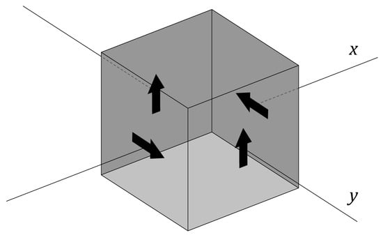
Figure 1.
A die (cube) with arrows on four sides and two possible axes of rotation. The die is rotated by about the x- or y-axis. The relevant outcome is the orientation of the arrow on the upper side: up (i.e., in the direction of the positive y-axis), right (in the direction of the positive x-axis), down, or left. From the depicted starting position, a rotation by about the x-axis (or y-axis) results in the arrow landing on top pointing up, while a rotation by yields the outcome down.
- A:
- The die is rotated with equal probability by or about the x-axis and we observe in which direction () the arrow on top is pointing.
- B:
- The die is rotated with equal probability by or about the y-axis and we observe in which direction the arrow on top is pointing.
If experiment A is performed first, followed by B, we have
All other outcomes have probability zero. If B is performed before A, we find
Again, all other outcomes (in particular and ) have probability zero. Thus, due to the non-commutativity of the rotations—corresponding here to the time evolutions of the initial state—the joint probability distribution of A and B depends on the order in which the measurements are carried out.
Such classical analogs go only so deep, but they can teach us where not to look for the profound innovations of quantum mechanics. For example, since pointed out by [22], much ado is made about the fact that the law of total probability
is violated for incompatible quantum observables. Well, we also find the alleged violation in our die example, e.g., (from (10)) while (from (11)). But the discrepancy is easily explained if we remember that the A-measurement performed first or alone would be described by a random variable of the form , while the A-measurement performed subsequently to the B-measurement is described by a random variable of the form . Here, and are rotations by about the x- and y-axis, respectively, which play the role of the dynamical flows in our measurement scheme. The point is that “” may denote the same macroevent in both cases, but it refers to different (and incompatible) measurements on the left- and right-hand side of (12), respectively. Really, a more careful notation would have sufficed to avoid any worries about the law of total probability. We merely found that , where and are different probability distributions pertaining to different experiments.
In less technical terms, the apparent violation of (12) is due to the fact that the B-measurement—specifically, the rotation about the y-axis—changes the state of the die in a way that affects the distribution of the subsequent A-measurement. Nothing more mysterious happens (at least not with regard to the law of total probability) if we consider, say, a z-spin measurement on an electron or an x-spin measurement followed by a measurement of its z-spin. Whatever the initial preparation, the x-spin measurement will change the quantum state of the electron (projecting it into an eigenstate of ) in a way that affects the distribution of the subsequent z-spin measurement. Averaging over the possible outcomes does not undo the effects of the x-spin measurement and will thus not recover the statistics of the first experiment.
Remark 1.
It is often claimed that non-commuting quantum observables do not have a joint probability distribution while “classical” random variables on a common probability space always do (e.g., [23]). We discussed why the joint probability distribution of random variables does not readily translate into the probability distribution of joint measurements. The first part of the claim is also misleading. Non-commuting observables have a well-defined joint distribution if one keeps track of the order of measurements ([24], pp. 166 ff).
2.3. Two Examples
Let us apply the Boltzmannian measurement scheme to concrete physical examples that illustrate the active role of the measurement process, as well as important (albeit special) cases in which it can be neglected.
Example 1.
Consider a classical N-particle gas in thermodynamic equilibrium at an unknown temperature T. In terms of Boltzmannian statistical mechanics, this means that the system’s microstate wanders around a macroregion of very large measure on which the value function
describing the average kinetic energy per particle, assumes an essentially constant value .
If we now bring this system (phase space ) in contact with a thermometer (phase space ), the joint system ( will quickly equilibrate to a common temperature . This value can be displayed on a thermometer scale by exploiting known relationships between temperature and certain material properties (say, the density of mercury or the resistance of an electrical conductor). If the gas has a much higher heat capacity than the thermometer, we have , so that the measurement result reflects, to a good approximation, the pre-measurement value of T and hence of the macrovariable (13) on . For practical purposes, the thermometer can thus be treated as a “passive” measurement device that indicates the temperature of the system.
However, in principle, all these thermodynamic arguments should be justified by a statistical mechanical analysis of the combined system gas + thermometer. If h is a macrovariable that describes, say, the level of mercury in the thermometer, the relevant result would take the form
where μ is the Liouville measure, the initial macrostate, Φ the dynamical flow that includes the interactions between gas and thermometer, and τ of the order of the system’s equilibration time.
This is about as close as it gets to an ideal thermodynamic measurement, for which the theory tells us that measurement outcomes reflect (to a good approximation) pre-measurement values of some state function. We do not have to look very far for classical experiments that are markedly different in this respect.
Example 2.
We consider a statistical mechanical description of a coin toss. Let Ω be the phase space of the coin’s microscopic constituents and the initial macrostate (which includes, in particular, the fact that the particles form a coin). We do not need a measurement device since we can directly observe which side of the coin lands on top. Denote by the macrostates corresponding to the coin coming to rest heads up and tails up, respectively. Let us assign the value to the outcome heads, and to tails. The corresponding value function is . Let be the flow resulting from the microscopic dynamics of our coin toss. The coin-toss experiment is then described by the random variable
and we call
the probability of the outcome , which should come out as (approximately) for a fair coin.
Assuming the statistical independence of repeated trials (which is very hard to justify from first principles), this probability distribution is all we need to make statistical predictions; the details of the function Z need not concern us. But it is crucial to note that different dynamics (i.e., different ways of tossing the coin) will, in general, give rise to different random variables (mappings from initial microstates to outcomes) even if they have the same probability distribution.
Consider a coin-toss experiment in which the microdynamics are the same as before, except that the coin is flipped over before reading off the result. This experiment would be described by a random variable that yields the same outcome probabilities as Z even though , i.e., the two random variables determine contradictory results for all possible initial microconditions.
As trivial as this last observation may be, it would suffice to prove a “no-hidden-variables theorem for coin tossing” whose upshot is similar to that of celebrated results in quantum mechanics: It is impossible to consistently assign predetermined outcome values independently of the details of the experiment (i.e., of how the coin is tossed). Of course, this has no profound implications whatsoever; it is a trivial consequence of the fact that the relevant outcomes are produced by the experiment, rather than reflecting an intrinsic property of a coin.
It turns out that, in this particular regard, measurements in quantum mechanics are more akin to tossing a coin than to taking the temperature. When we send a photon through a polarization filter, we do not measure a pre-existing polarization but make the photon pick one (so to speak). The disanalogies may be more numerous and striking (phenomena such as interference, entanglement, or the repeatability of (ideal) measurements, which are all related to the wave function). But this makes it only more peculiar that so much of the hidden variables debate revolves around an aspect of quantum measurements—their active role in bringing about outcomes—that is quite mundane and easily reproduced by classical experiments.
3. Boltzmannian Analysis of No-Go Theorems
How much more is there to the (in)famous no-hidden-variables theorems in quantum mechanics? To find out, let us analyze them from the perspective of Boltzmannian statistical mechanics, applying the technical and conceptual framework introduced above.
In essence, theorems of the Kochen–Specker type aim to prove that there is no “good” map from observable operators on some Hilbert space to random variables on some probability space , such that
i.e., the possible values of correspond to eigenvalues of , and
for an appropriate probability measure , reproducing the statistical predictions of quantum mechanics for the quantum state . Note that can be a projector (into an eigenspace of some other observable), in which case the left-hand side of (18) is the quantum mechanical probability of the respective measurement outcome. In fact, since every self-adjoint operator has a spectral decomposition, it suffices to require (18) for projectors.
As Kochen and Specker [3] point out, it is always possible to construct some such map together with a suitable probability space . No-go theorems thus need additional assumptions on what constitutes a “good” one.
The Kochen–Specker theorem requires
for commuting operators so that the algebraic structure is respected for compatible observables. This is the formal expression of noncontextuality (the terminology will become clearer soon). For a simple impossibility proof due to Mermin [7], consider the following scheme of observables (from now on, I omit the “hats”):
The following properties are easily verified using the commutation rules for Pauli matrices:
- (a)
- All observables have the eigenvalues and .
- (b)
- The observables along each column and each row commute.
- (c)
- The product along each row is 1.
- (d)
- The product along the first column and along the second column is 1, while the product along the third column is .
Hence, it is impossible to assign values to all nine observables in a consistent manner, as a family of random variables satisfying (19) would have to. (The product of all nine values would have to be according to (c), but according to (d)). Hence, hidden variables are a “no go”. Or are they?
3.1. Who’s Afraid of Contextuality?
The composition rules (19) are the critical premise of the theorem. Notably, they could not be contentious whatsoever if they simply meant: we measure (or ) by measuring A and measuring B and then multiplying (adding) the two results. In other words, (19) would be a harmless triviality if “measuring the product of commuting observables” always meant the physical operation of measuring the observables individually followed by the mathematical operation of taking the product of the respective outcomes. (Ditto for the sum).
But this cannot be what “measuring ” means when is measured together with the observables and , which do not commute, i.e., are incompatible, with A and B individually. The measurement of in the first “context”—together with A and B, as in the leftmost column of (20)—is simply a matter of multiplying the results obtained for A and B. The measurement of in the second context—together with and , as in the third row of (20)—requires an entirely different method. It is not obvious what that method is (or whether the respective measurement is feasible at all), but it would amount to an entirely different experiment involving different interactions with the particles.
Consequently, the two experiments would have to be described by different random variables (on the state space of the hypothetical “hidden” microvariables), which we denote by and , respectively. At best, they will be of the form and with identical value functions but different time evolutions . These random variables may have the same (marginal) distribution, but will generally correspond to different mappings from initial microstates (in terms of the hidden variables) to measurement outcomes. Indeed, it could even easily happen that for all , as the trivial coin toss example in Section 2.3 demonstrates.
From these considerations alone, we should expect
i.e., a violation of (19) in the second context. The same applies to other product observables in (20) that would have to be measured in incompatible “contexts” corresponding to their row and column, respectively.
To be clear, it is possible that different dynamics evolve all (or most) initial microstates into the same final macrostates, thus resulting in (more or less) the same random variable. Since v is coarse-graining, and could define the same function on (or at least on the initial macroregion ) even if . However, unless we have convergence to a dominant equilibrium state, this is not the generic case. (Convergence to equilibrium is very robust against the details of the microscopic dynamics because the equilibrium region exhausts almost the entire phase space volume [15]). (almost everywhere) is a much more stringent condition than equivalence in distribution, and noncontextuality requires the former.
From this perspective, the Kochen–Specker theorem is not a great improvement over von Neumann’s no-go theorem [25], which John Bell famously characterized as “silly” [26] (although some recent reappraisals have been more generous [27,28,29]). Von Neumann’s theorem required that nice composition rules—specifically the additive one in (19)—hold even for non-commuting observables. (It is then easy to see that random variables as in (17) cannot exist. For example, considering the non-commuting spin-observables and , we have , i.e., the eigenvalues of their sum are not sums of their eigenvalues). As Bell [8] pointed out, this amounts to the unjustified assumption that relations between random variables, which need to hold only in expectation (since the expectation values of quantum observables are additive), must also hold pointwise, even when these variables describe different and mutually incompatible experiments. The Kochen–Specker theorem requires (19) only for commuting observables, but this nonetheless amounts to assuming that identities between random variables, which need to hold only in distribution, must hold pointwise, even though they correspond to different and incompatible experiments. The impact of the resulting impossibility proof then comes, at least in part, from packaging this unjustified assumption into the concept of “noncontextuality” and implying that a violation of “noncontextuality” is somehow bad. In fact, we just saw that it is an almost trivial feature of random variables describing measurement experiments.
The Kochen–Specker theorem still accomplishes something. What it convincingly disproves is not hidden variables but “naive realism about operators” [30], more specifically the idea that eigenvalues of observable operators correspond to intrinsic properties of the measured system. In that case, (19) would be justified, at least for idealized measurements that cause a negligible disturbance of the measured quantity. However, it turns out that “spin measurements”, for instance, do not simply measure an intrinsic “spin”. First and foremost, the experiments observe the reaction of a particle to a magnetic field (and subsequent detection, e.g., at a screen). In a hidden variables theory, the state of the particle does not have to determine the respective outcomes independently of the details of the experiment (cf. [31]), any more than the complete microstate of a coin has to determine the outcome of a coin toss independently of how the coin is tossed. Ultimately, the hidden variables theory would have to tell us which, if any, observables correspond to intrinsic quantities that can be revealed by appropriate measurements (in Bohmian mechanics, for example, it is only position). Reifying an entire observable algebra a priori thus begs the question against the hidden variables program.
The Boltzmannian analysis does not leave much mystery around no-go results of the Kochen–Specker type, but it does leave some open questions. In particular, one may ask: Why should all these different experiments, which are associated with the same observable operator, have the same statistical features unless they all measured the same physical quantity? An interesting answer is suggested by the Bohmian analysis of the measurement process [32]. It is really the other way around: different measurement experiments are associated with the same operator because they have the same statistics (which, in turn, might be constrained by certain symmetries, for example). We could call every experiment that produces independent 50:50 chances a “coin toss”, but it would be absurd to infer that there must be some physical quantity that they are all trying to measure.
3.2. Why Bell’s Theorem Is Not Silly
We consider the “non-probabilistic” version of Bell’s theorem, based on the GHZ experiment [33,34], as this makes comparisons with Kochen–Specker-type results more straightfoward. The experiment concerns three spin-1/2 particles in the entangled state
and the four mutually commuting observables
The following facts are straightforwardly verified:
- (a)
- is an eigenstate of with eigenvalue .
- (b)
- is an eigenstate of with eigenvalue .
Whichever of the four experiments is carried out, given the outcomes of two of the spin measurements involved, we can immediately infer the outcome of the third. And yet, it is impossible to consistently assign predetermined values such that , etc. On the one hand, (a) and (b) imply that the product must be . On the other hand, since each of the six Pauli matrices appears exactly twice in (23), it would have to be the product of the squares of the six values and thus identical to .
An important observation is that (etc.) can and should be read as a definition. No assumption of non-contextuality in form of (19) is needed here, since, unlike in the KS scenario, the relevant experiment can always be performed by carrying out individual measurements on the three particles and then multiplying the results.
Nonetheless, the impossibility proof implies that at least one of the following identities must fail (though it is most plausible to assume that all of them do):
As before, denotes the random variable (on some state space ) that describes the measurement of if it occurs together with the measurements of and . It is thereby implicitly assumed that the parameter settings, specifying which measurements are performed, are independent of the microstates on which the random variables are defined (Bell’s “no conspiracy” condition).
The failure of (24) is analogous to (21) in our analysis of the Mermin–Kochen–Specker scenario. If, say, , it means that measuring together with and or measuring together with and amounts to different experiments with different dynamics. In this sense, we have another instance of contextuality. But in contrast to the Kochen–Specker scenario, it is indeed remarkable. It is extremely remarkable if the three measurements—including free parameter choices for the directions of the spin measurements—occur at such a large spatial and such a short temporal distance that they could only influence each other superluminally. Then, tells us that the dynamical evolution of the microvariables describing particle 1 and its measurement must have some nonlocal dependence on the distant measurements performed on particles 2 and 3. This nonlocality was precisely Bell’s point.
I conclude this section with a few important remarks.
Remark 2.
- As indicated above, nonlocality can be regarded as a special case of contextuality, as it entails that the value of one observable cannot be predetermined independently of which other (compatible) observables are measured alongside it. It is therefore sometimes suggested that the key improvement of Bell-type theorems over KS-type theorems is that they provide a better justification for expecting non-contextuality, namely the locality assumption (together with the spacelike separation of the pertinent measurements), which implies that the measurements cannot disturb each other [7]. This framing overlooks the crucial point that the definition of non-contextuality relies on the algebraic structure of quantum observables, whereas Bell-locality is not about observable operators at all. The former assumption, underlying the KS theorem, proves gratuitous in a hidden-variables framework in which observable operators are no longer fundamental. A violation of locality, in contrast, has profound dynamical implications for any theory that seeks to reproduce the predictions of quantum mechanics.
- In the Boltzmannian framework, it is most natural to think of the failure of (24) as a violation of “parameter independence”, meaning that, e.g., depends on what measurements (x-spin or y-spin) are performed on the other two particles. These correspond, after all, to different settings of the Stern–Gerlach magnet (or polarizer, in the case of photons) and thus to different interactions with the particles. However, in principle, we could also reproduce the quantum predictions for the GHZ experiment by allowing to depend on the outcomes (but not the parameter choices) for the other two other measurements. This should not be confused with the innocuous observation that the measurement results are correlated. Random variables that violate “outcome independence” would still mean that the dynamical evolution of the state variables describing a particle and its measurement is nonlocally influenced by distant events.
- Finally, one should emphasize that Bell’s theorem (especially in its 1990 version [2]) is more general than the argument discussed here and does not presuppose the Boltzmannian framework. Our analysis merely corroborates (and perhaps further elucidates) Bell’s finding that the nonlocality of quantum mechanics cannot be cured by additional variables.
4. Misleading Terminology
The muddled debate about no-hidden-variables theorems in quantum mechanics is also a story of misleading terminology. For the preceding discussion, I largely adopted the established jargon myself, though I tried to minimize its harm.
The first and foremost piece of misleading terminology is the term “hidden variables” itself. It suggests some spurious theoretical structure that “secretly” determines observable values but has no direct link to empirical observation. In contrast, the microvariables in Boltzmannian statistical mechanics must coarse grain, in a straightforward sense, to the “measurement outcomes” as registered by macroscopic instruments. At the same time, it is assumed that our epistemic access to the microvariables is limited; that we empirically discern macrostates rather than microstates. Still, this does not change the fact that observing the expansion of a gas or the rising mercury levels on a thermometer is to observe a collection of particles in a determinate microscopic state.
There are independent reasons to believe that precisely such variables are missing in quantum mechanics, that the wave function or quantum state is not the right kind of theoretical object to make contact with observable reality. Defending this claim is beyond the scope of this paper; it suffices to note that it is a common motivation behind attempts to complete quantum mechanics with additional variables and that it would defeat the purpose if these variables were truly hidden ([35], Ch. 1). The additional variables should rather play the role of what Bell dubbed local beables ([4], Ch. 7), or what has become known in the literature as a primitive ontology (see, e.g., [36,37,38]).
The theory might impose limits on the accuracy with which the respective microstates can be observed and prepared—indeed, it has to if it is not to allow violations of cherished principles of quantum mechanics. But this is similar to the reduction of thermodynamics by classical statistical mechanics, which implies that we could violate the second law of thermodynamics if we had sufficient control over microscopic degrees of freedom. The situation is, in fact, more satisfying in existing primitive ontology quantum theories, where the relevant epistemic limits are not assumed but derived [39,40].
The next example of deceptive language is the misuse of the word “measurement” that Bell already complained about.
This word very strongly suggests the ascertaining of some preexisting property of some thing, any instrument involved playing a purely passive role. Quantum experiments are simply not like that, as we learned especially from Bohr. The results have to be regarded as the joint product of ’system’ and ’apparatus’, the complete experimental set-up. But the misuse of the word ’measurement’ makes it easy to forget this and then to expect that the ’results of measurements’ should obey some simple logic in which the apparatus is not mentioned. The resulting difficulties soon show that any such logic is not ordinary logic. It is my impression that the whole vast subject of ’Quantum Logic’ has arisen in this way from the misuse of a word. I am convinced that the word ’measurement’ has now been so abused that the field would be significantly advanced by banning its use altogether, in favour for example of the word ’experiment’. ([4], p. 166)
This brings me to my final example of misleading terminology, which is the slapping-on of the prefixes “classical” and “quantum” to terms like “logic” or “probability theory”. In a loose sense, “quantum probability theory” can simply mean the application of the quantum formalism to make probabilistic predictions. In a stricter sense, it refers to an even more abstract framework built around the quantum formalism as an alleged alternative to (or generalization of) Kolmogorov’s “classical probability theory” and its underlying Boolean logic (see, e.g., [41] for an overview and [42] for a defense). In any case, the name easily suggests that “classical probability theory” is somehow the probability theory of classical mechanics and has been superseded after the development of quantum theory. The last part of this suggestion is highly questionable; the first is plainly wrong. While probability theory has proven exceedingly successful in classical statistical mechanics, it does not hinge on either the laws or the ontology of Newtonian physics. Admittedly, there is a sense in which probability theory presupposes some ontology as the subject of probabilistic reasoning, which might put it at odds with (Neo-)Copenhagen interpretations of quantum mechanics. As Erwin Schrödinger already lamented in a letter to Einstein:
It seems to me that the term “probability” is often abused nowadays. […] A probability statement presupposes the full reality of its subject. No reasonable person will make a guess as to whether Caesar’s die at the Rubicon had a five on top. The quantum mechanists sometimes pretend that probability statements are to be applied especially to events with a blurred reality. (Schrödinger to Einstein. November 18, 1950. Letter 238 in ([43], pp. 627–629). (My translation).
More than the general analysis provided in this paper, theories like Bohmian mechanics are proof positive that no quantum phenomena compel us to give up on standard probability theory. The argument for doing so nonetheless would have to be that it allows for better, deeper, more coherent explanations. I believe quantum probability theory is doing quite the opposite—that it is just another layer of abstraction, weaved around an instrumentalist formalism, which takes us further away from any physical content—but prosecuting this charge would take a separate discussion.
5. Conclusions
From a purely technical point of view, one can appreciate “no-go” theorems as neat mathematical results that foreclose parts of the logical space for possible extensions or modifications of quantum mechanics. Their physical and philosophical relevance, however, depends on how compelling the theorems’ assumptions are; how plausible or attractive it was to explore the foreclosed regions of logical space in the first place. This is not always obvious, as the physical meaning of mathematical premises can be more or less obscure.
Bell-type theorems are so profound because (a) locality and no-conspiracy are very compelling assumptions, (b) their mathematical formalization by Bell is transparent and does not hinge on the quantum measurement formalism, and (c) because the kind of nonlocality that comes with quantum entanglement is indeed a (if not the) revolutionary feature of quantum theory. The Kochen–Specker assumption of noncontextuality may seem plausible at the level of abstraction at which the theorem is generally formulated. However, a more careful statistical–mechanical analysis has shown that contextuality is a typical feature of random variables describing measurement experiments and, indeed, unavoidable when the measurement process plays an active role in bringing about the relevant outcomes, as is certainly the case for most quantum measurements. This corroborates the conclusion of [8] that no-hidden-variables theorems of the KS-type are based on unreasonable assumptions. It also means that these theorems fall short of capturing a genuinely “non-classical” feature of quantum statistics.
As argued in Section 1, the dialectic of the entire hidden-variables debate is strangely off, and it is unclear how the so-called no-hidden-variables theorems support an argument against the hidden-variables program. A hidden-variables theory cannot assign predetermined values to larger classes of quantum observables, but neither does standard quantum mechanics. A non-conspiratorial hidden-variables theory must violate Bell-locality, but standard quantum mechanics violates it already, as Bell himself emphasized.
If the respective no-go results are supposed to tip the scale either way, then maybe by asking what (type of) theory best elucidates their physical meaning could help clarify matters. Here, it was shown that the theorems can be well understood within the framework of Boltzmannian statistical mechanics (which fits, in particular, Bohmian mechanics as the prime example of a primitive ontology quantum theory). I leave the reader with the question of whether orthodox quantum mechanics has provided a better understanding or rather shrouded the results in unnecessary mystery and confusion.
Funding
This research was supported by the ISRAEL SCIENCE FOUNDATION (grant No. 1597/23).
Data Availability Statement
No new data were created or analyzed in this study.
Acknowledgments
Thanks to Avi Levy and Christian Beck for valuable discussions and to anonymous referees for helpful comments.
Conflicts of Interest
The author declares no conflicts of interest.
References
- Bell, J.S. On the Einstein Podolsky Rosen Paradox. Physics 1964, 1, 195–200. [Google Scholar] [CrossRef]
- Bell, J.S. La Nouvelle Cuisine. In Between Science and Technology; Sarlemijn, A., Kroes, P., Eds.; Elsevier Science: Amsterdam, The Netherlands, 1990. [Google Scholar]
- Kochen, S.; Specker, E.P. The Problem of Hidden Variables in Quantum Mechanics. J. Math. Mech. 1967, 17, 59–87. [Google Scholar] [CrossRef]
- Bell, J.S. Speakable and Unspeakable in Quantum Mechanics, 2nd ed.; Cambridge University Press: Cambridge, UK, 2004. [Google Scholar]
- Norsen, T. John S. Bell’s Concept of Local Causality. Am. J. Phys. 2011, 79, 1261–1275. [Google Scholar] [CrossRef]
- Maudlin, T. What Bell Did. J. Phys. A Math. Theor. 2014, 47, 424010. [Google Scholar] [CrossRef]
- Mermin, N.D. Hidden Variables and the Two Theorems of John Bell. Rev. Mod. Phys. 1993, 65, 803–815. [Google Scholar] [CrossRef]
- Bell, J.S. On the Problem of Hidden Variables in Quantum Mechanics. Rev. Mod. Phys. 1966, 38, 447–452. [Google Scholar] [CrossRef]
- Maudlin, T. Three Measurement Problems. Topoi 1995, 14, 7–15. [Google Scholar] [CrossRef]
- Bohm, D. A Suggested Interpretation of the Quantum Theory in Terms of “Hidden” Variables. II. Phys. Rev. 1952, 85, 180–193. [Google Scholar] [CrossRef]
- Heisenberg, W. Physics and Beyond: Encounters and Conversations; Harper & Row: New York, NY, USA, 1971. [Google Scholar]
- Lazarovici, D.; Oldofredi, A.; Esfeld, M. Observables and Unobservables in Quantum Mechanics: How the No-Hidden-Variables Theorems Support the Bohmian Particle Ontology. Entropy 2018, 20, 381. [Google Scholar] [CrossRef]
- Schilpp, P.A. (Ed.) Albert Einstein: Philosopher-Scientist, 1st ed.; Number VII in the Library of Living Philosophers; The Library of Living Philosophers Inc.: Evanston, IL, USA, 1949. [Google Scholar]
- Goldstein, S. Boltzmann’s Approach to Statistical Mechanics. In Chance in Physics: Foundations and Perspectives; Bricmont, J., Dürr, D., Galavotti, M.C., Ghirardi, G., Petruccione, F., Zanghì, N., Eds.; Springer: Berlin/Heidelberg, Germany, 2001; pp. 39–54. [Google Scholar]
- Lazarovici, D. Typicality Reasoning in Probability, Physics, and Metaphysics; New Directions in the Philosophy of Science; Palgrave Macmillan: Cham, Switzerland, 2023. [Google Scholar] [CrossRef]
- Spekkens, R.W. Contextuality for Preparations, Transformations, and Unsharp Measurements. Phys. Rev. A 2005, 71, 052108. [Google Scholar] [CrossRef]
- Dürr, D.; Teufel, S. Bohmian Mechanics: The Physics and Mathematics of Quantum Theory; Springer: Berlin/Heidelberg, Germany, 2009. [Google Scholar]
- Dürr, D.; Goldstein, S.; Zanghì, N. Quantum Physics without Quantum Philosophy; Springer: Berlin/Heidelberg, Germany, 2013. [Google Scholar]
- Hemmo, M.; Shenker, O.R. The Road to Maxwell’s Demon: Conceptual Foundations of Statistical Mechanics; Cambridge University Press: Cambridge, UK, 2012. [Google Scholar] [CrossRef]
- Frauchiger, D.; Renner, R. Quantum Theory Cannot Consistently Describe the Use of Itself. Nat. Commun. 2018, 9, 3711. [Google Scholar] [CrossRef] [PubMed]
- Lazarovici, D.; Hubert, M. How Quantum Mechanics Can Consistently Describe the Use of Itself. Sci. Rep. 2019, 9, 470. [Google Scholar] [CrossRef]
- Feynman, R.P. Space-Time Approach to Non-Relativistic Quantum Mechanics. Rev. Mod. Phys. 1948, 20, 367–387. [Google Scholar] [CrossRef]
- Fine, A. Joint Distributions, Quantum Correlations, and Commuting Observables. J. Math. Phys. 1982, 23, 1306–1310. [Google Scholar] [CrossRef]
- Beck, C. Local Quantum Measurement and Relativity; Fundamental Theories of Physics; Springer International Publishing: Cham, Switzerland, 2021; Volume 201. [Google Scholar] [CrossRef]
- von Neumann, J. Mathematische Grundlagen der Quantenmechanik; Springer: Berlin/Heidelberg, Germany, 1932. [Google Scholar] [CrossRef]
- Bell, J.S. Interview: John Bell. Omni 1988, 1988, 85–92. [Google Scholar]
- Bub, J. Von Neumann’s `No Hidden Variables’ Proof: A Re-Appraisal. Found. Phys. 2010, 40, 1333–1340. [Google Scholar] [CrossRef]
- Dieks, D. Von Neumann’s Impossibility Proof: Mathematics in the Service of Rhetorics. Stud. Hist. Philos. Sci. Part B Stud. Hist. Philos. Mod. Phys. 2017, 60, 136–148. [Google Scholar] [CrossRef]
- Acuña, P. Von Neumann’s Theorem Revisited. Found. Phys. 2021, 51, 73. [Google Scholar] [CrossRef]
- Daumer, M.; Dürr, D.; Goldstein, S.; Zanghì, N. Naive Realism about Operators. Erkenntnis 1996, 45, 379–397. [Google Scholar] [CrossRef]
- Norsen, T. The Pilot-Wave Perspective on Spin. Am. J. Phys. 2014, 82, 337–348. [Google Scholar] [CrossRef]
- Dürr, D.; Goldstein, S.; Zanghì, N. Quantum Equilibrium and the Role of Operators as Observables in Quantum Theory. J. Stat. Phys. 2004, 116, 959–1055. [Google Scholar] [CrossRef]
- Greenberger, D.M.; Horne, M.A.; Zeilenger, A. Going Beyond Bell’s Theorem. In Bell’s Theorem, Quantum Theory and Conceptions of the Universe; Kafatos, M., Ed.; Kluwer Academic Publishers: Dodrecht, The Netherlands, 1989; pp. 69–72. [Google Scholar]
- Mermin, N.D. What is Wrong with These Elements of Reality? Phys. Today 1990, 43, 9–11. [Google Scholar] [CrossRef]
- Bohm, D.; Hiley, B.J. The Undivided Universe. An Ontological Interpretation of Quantum Theory; Routledge: London, UK, 1993. [Google Scholar]
- Allori, V.; Goldstein, S.; Tumulka, R.; Zanghì, N. On the Common Structure of Bohmian Mechanics and the Ghirardi-Rimini-Weber Theory. Br. J. Philos. Sci. 2008, 59, 353–389. [Google Scholar] [CrossRef]
- Esfeld, M. From the Measurement Problem to the Primitive Ontology Programme. In Do Wave Functions Jump? Perspectives of the Work of GianCarlo Ghirardi; Allori, V., Bassi, A., Dürr, D., Zanghi, N., Eds.; Springer Nature: Cham, Switzerland, 2020; pp. 95–108. [Google Scholar]
- Lazarovici, D.; Reichert, P. The Point of Primitive Ontology. Found. Phys. 2022, 52, 120. [Google Scholar] [CrossRef]
- Dürr, D.; Goldstein, S.; Zanghì, N. Quantum Equilibrium and the Origin of Absolute Uncertainty. J. Stat. Phys. 1992, 67, 843–907. [Google Scholar] [CrossRef]
- Cowan, C.W.; Tumulka, R. Epistemology of Wave Function Collapse in Quantum Physics. Br. J. Philos. Sci. 2016, 67, 405–434. [Google Scholar] [CrossRef][Green Version]
- Wilce, A. Quantum Logic and Probability Theory. In The Stanford Encyclopedia of Philosophy; Fall 2021 ed.; Zalta, E.N., Ed.; Metaphysics Research Lab, Stanford University: Stanford, CA, USA, 2021. [Google Scholar]
- Pitowsky, I. Quantum Mechanics as a Theory of Probability. In Physical Theory and Its Interpretation: Essays in Honor of Jeffrey Bub; Demopoulos, W., Pitowsky, I., Eds.; Springer: Dordrecht, The Netherlands, 2006; pp. 213–240. [Google Scholar] [CrossRef]
- von Meyenn, K. (Ed.) Eine Entdeckung von ganz Außerordentlicher Tragweite: Schrödingers Briefwechsel zur Wellenmechanik und zum Katzenparadoxon; Springer: Berlin/Heidelberg, Germany, 2011. [Google Scholar] [CrossRef]

Disclaimer/Publisher’s Note: The statements, opinions and data contained in all publications are solely those of the individual author(s) and contributor(s) and not of MDPI and/or the editor(s). MDPI and/or the editor(s) disclaim responsibility for any injury to people or property resulting from any ideas, methods, instructions or products referred to in the content. |
© 2024 by the author. Licensee MDPI, Basel, Switzerland. This article is an open access article distributed under the terms and conditions of the Creative Commons Attribution (CC BY) license (https://creativecommons.org/licenses/by/4.0/).