Diffusion in a Comb-Structured Media: Non-Local Terms and Stochastic Resetting

Abstract

We examine the dynamics of a system influenced by a backbone structure, incorporating linear non-local terms that account for both irreversible and reversible processes, such as absorption and adsorption–desorption. Additionally, we introduce stochastic resetting to analyze its effects on the system’s behavior from both analytical and numerical perspectives. Our findings reveal a rich spectrum of dynamics, emphasizing connections to anomalous diffusion and providing new insights into transport phenomena in complex environments.

1. Introduction

Diffusion is one of nature’s most fundamental transport processes, occurring in a broad spectrum of systems, including porous rocks [1], monoclonal antibody diffusion [2], electrical impedance [3], nematode locomotion [4], lithium-anion clusters in ionic liquids [5], colloidal motion [6], and heterogeneous membranes [7]. The ubiquity of diffusion is deeply related to the diversity of stochastic processes that govern it, ranging from classical (Markovian) to memory-dependent (non-Markovian) dynamics [8,9]. In conventional Brownian diffusion, the mean square displacement (MSD) follows a linear time scaling $\langle {\left(\Delta x\right)}^2\rangle$∼t. However, many complex systems exhibit anomalous diffusion, where MSD can obey a power law, e.g., $\langle {\left(\Delta x\right)}^2\rangle$∼$t^{\alpha }$, with $\alpha <1$ indicating subdiffusion and $\alpha >1$ corresponding to superdiffusion [10,11]. Beyond these regimes, other transport behaviors emerge, such as ultra-slow diffusion, where MSD can depend logarithmically on time, $\langle {\left(\Delta x\right)}^2\rangle$∼${ln}^{\sigma }t$ [12,13,14], or be characterized by accelerated growth, $\langle {\left(\Delta x\right)}^2\rangle$∼$t^{2+\lambda }$ for $1\le \lambda \le 3$ [15], which corresponds to hyperdiffusion.

To describe these diverse diffusion scenarios, various mathematical frameworks have been developed, including generalized Langevin equations [16,17], master equations [18,19], power Brownian motion [20] (see also the Refs. [21,22] about the power Lévy motion), random walk models [23,24], and fractional Fokker–Planck equations [25,26,27]. Among these approaches, the comb model has been successfully applied to analyze the diffusion process and capture the behavior in systems with geometric constraints. It is characterized by a backbone structure with branches or teeth, which restricts the movement and usually results in subdiffusive transport along the backbone. This model is particularly pertinent for describing transport phenomena in disordered and biological systems, such as percolation clusters [28,29], effective medium approximations [30], quantum systems [31,32], and spiny dendrites [33].

The standard form of the comb model in two dimensions is described by the following diffusion equation [34]:

$$\begin{array}{c}\hfill {\displaystyle \frac{\partial }{\partial t}}\rho (\mathbf{r},t)={\mathcal{D}}_x\delta \left(y\right){\displaystyle \frac{{\partial }^2}{\partial x^2}}\rho (\mathbf{r},t)+{\mathcal{D}}_y{\displaystyle \frac{{\partial }^2}{\partial y^2}}\rho (\mathbf{r},t),\end{array}$$

(1)

with $\mathbf{r}=(x,y)$, where the delta function restricts the diffusion along the backbone (x-direction), while diffusion in the y-direction represents motion along the branches. This formulation naturally introduces anisotropic and subdiffusive behavior along the backbone, i.e., in the x direction. This point can be verified by the reduced distributions that emerge from Equation (1) for the x variable and can be connected with the solutions of a fractional diffusion equation with index $1/2$ [35]. This feature leads us to obtain the mean square displacement ${\sigma }_x^2\sim t^{1/2}$ (subdiffusion), and the stochastic process related to this model is a subordinated Brownian motion [8]. Extensions of the comb model have incorporated additional complexities, such as fractional differential operators [34], heterogeneous media [36], dual-phase-lag models [37], stochastic resetting [38,39,40], reaction–diffusion dynamics [41,42,43], and Lévy flights [44]. These modifications introduce different aspects and bring new possibilities to understand diffusion in complex environments.

Here, we analyze an extension of the standard comb model by incorporating non-local terms and stochastic resetting to capture additional mechanisms that are not present in the previous models. This analysis is performed from analytical and numerical points of view. The equation considered is given by

$$\begin{array}{c}\hfill \begin{array}{cc}\hfill {\displaystyle \frac{\partial }{\partial t}}\rho (\mathbf{r},t)={\mathcal{D}}_x& \delta \left(y\right){\displaystyle \frac{{\partial }^2}{\partial x^2}}\rho (\mathbf{r},t)+{\mathcal{D}}_y{\displaystyle \frac{{\partial }^2}{\partial y^2}}\rho (\mathbf{r},t)-\mathcal{R}(\mathbf{r},t)\hfill \\ & +\eta \left(\mathcal{S}\left(t\right)\delta (\mathbf{r}-{\mathbf{r}}^{\prime })-\rho (\mathbf{r},t)\right),\hfill \end{array}\end{array}$$

(2)

where $\mathcal{S}\left(t\right)={\int }_{-\infty }^{\infty }dy{\int }_{-\infty }^{\infty }dx\rho (\mathbf{r},t)$. and the term $\mathcal{R}(\mathbf{r},t)$ is given by

$$\begin{array}{c}\hfill \begin{array}{cc}\hfill \mathcal{R}(\mathbf{r},t)=& \delta \left(y\right){\int }_0^{t}d{t}^{\prime }{\mathfrak{K}}_{1,x}(t-t^{\prime })\rho (\mathbf{r},t^{\prime })+\delta \left(y\right)\delta \left(x\right){\int }_0^{t}d{t}^{\prime }\mathfrak{K}(t-t^{\prime })\rho (\mathbf{r},t^{\prime })\hfill \\ & -\delta \left(y\right){\int }_0^{t}d{t}^{\prime }{\int }_{-\infty }^{\infty }d{x}^{\prime }{\mathfrak{K}}_{2,x}(x-x^{\prime },t-t^{\prime }){\displaystyle \frac{{\partial }^2}{\partial x^{\prime 2}}}\rho (\mathbf{r},t^{\prime }).\hfill \end{array}\end{array}$$

(3)

Equation (2) is closely related to the comb model [29,39,45,46,47], where the delta function in the diffusive term imposes a backbone structure restricting diffusion along the x-direction, and the diffusion in the y-direction corresponds to the branches (see Figure 1). The non-local terms in Equation (3) may describe memory effects and long-range interactions, which depend on the choice of the kernels ${\mathfrak{K}}_{1,x}(x,t)$, ${\mathfrak{K}}_{2,x}(x,t)$, and $\mathfrak{K}\left(t\right)$. These terms may also model different types of heterogeneous media and anomalous transport behaviors. In particular, the last term of Equation (3) can be combined with the diffusive term in the x direction, leading us to a fractional spatial derivative of distributed order when, e.g., ${\mathfrak{K}}_{2,x}(x,t)={\mathfrak{K}}_{2,x}\left(x\right)\delta \left(t\right)$. The last term in Equation (2) accounts for stochastic reset [48,49,50]. The presence of the survival probability, $\mathcal{S}\left(t\right)$, takes into account the particles present in the system. In fact, the particles may be trapped or absorbed by the nonlocal terms or boundary conditions, which may adsorb or absorb the particles of the systems. Similar to the standard comb model, the stochastic process related to this model, i.e., Equation (2) combined with Equation (3), can also be related with a subordinated Brownian motion [8] in a more complex scenario due to the presence of the nonlocal terms. To analyze Equation (2), we first consider the effect of non-local terms in the absence of stochastic reset. Following, we incorporate the stochastic resetting in the previous scenario by considering first the effects produced only by the backbone structure and, afterward, the presence of the non-local terms. These developments consider the combination of different effects for the diffusion process of a system and allow us to analyze the interplay among them. In this sense, it is worth mentioning that the geometric aspect of the comb model with the additional terms considered here may be connected with several physical and biological systems. For example, in neurobiology, the backbone-and-teeth (branches) structure resembles spiny dendrites in neurons, where molecular diffusion and transient trapping in dendritic spines have resulted in anomalous subdiffusion [51,52], to tracer transport in porous geological media [1,53], and nuclear transport of DNA-binding proteins [54,55]. In this manner, the analysis that emerges when different effects are combined opens the possibility of covering various scenarios where different aspects can be manifested.

The plan of this work is as follows: Section 2 presents formal results for Equation (2) in the absence and presence of the stochastic resetting; Section 3 shows numerical developments for Equation (2); and in Section 4, we present our discussion and conclusions

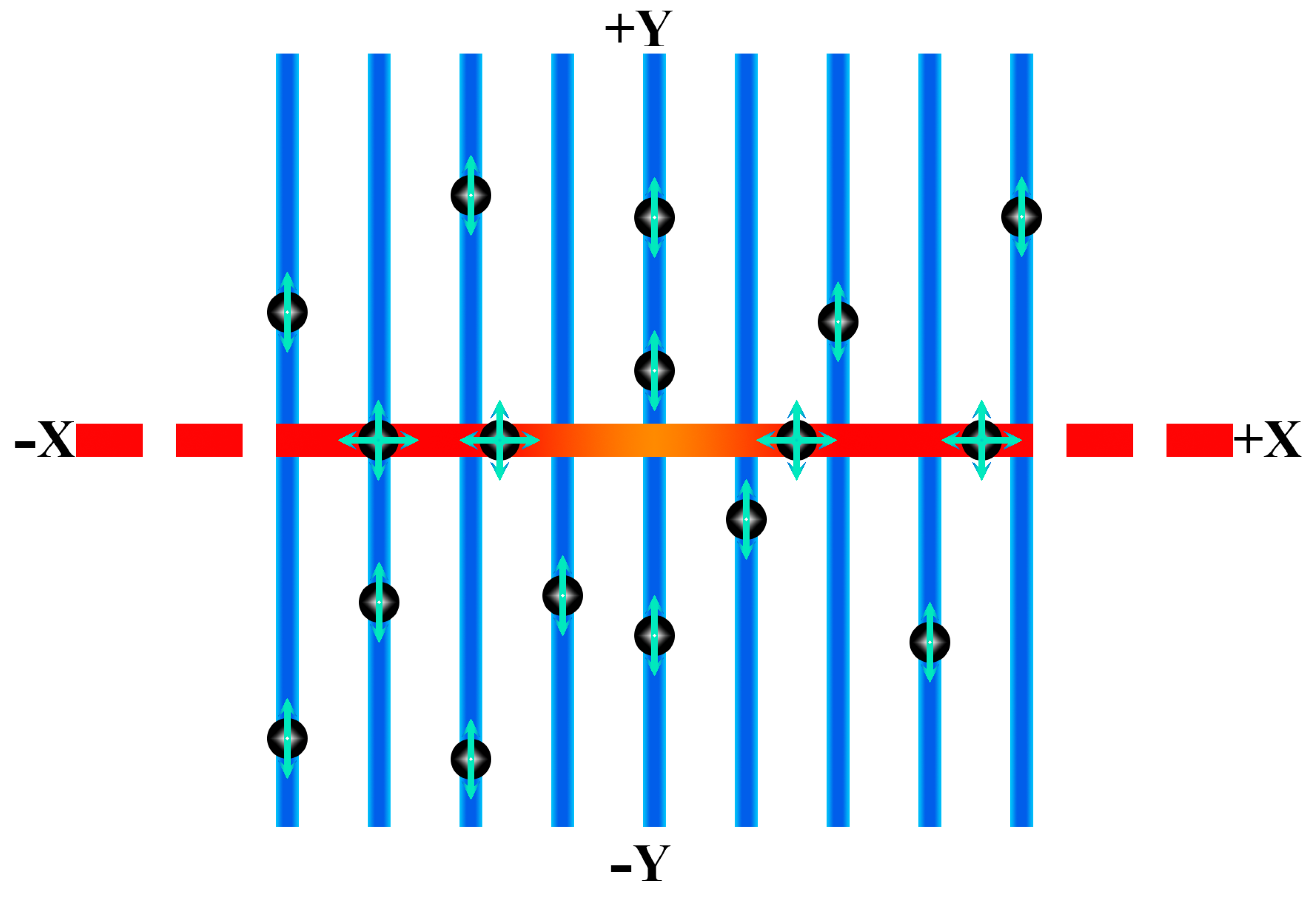
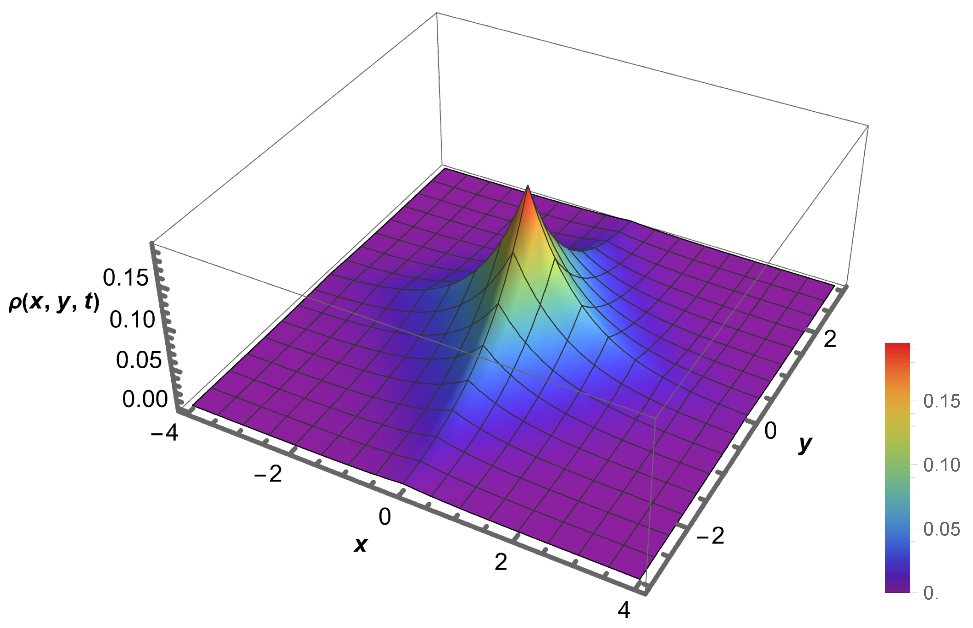
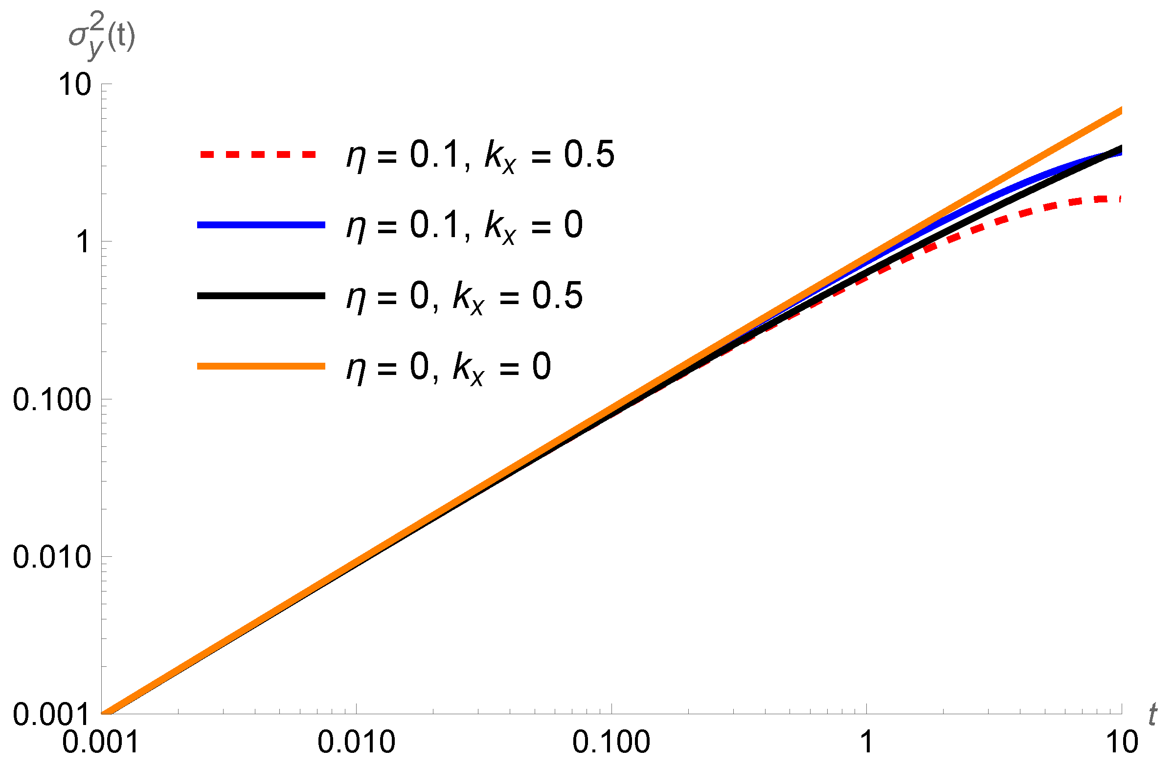
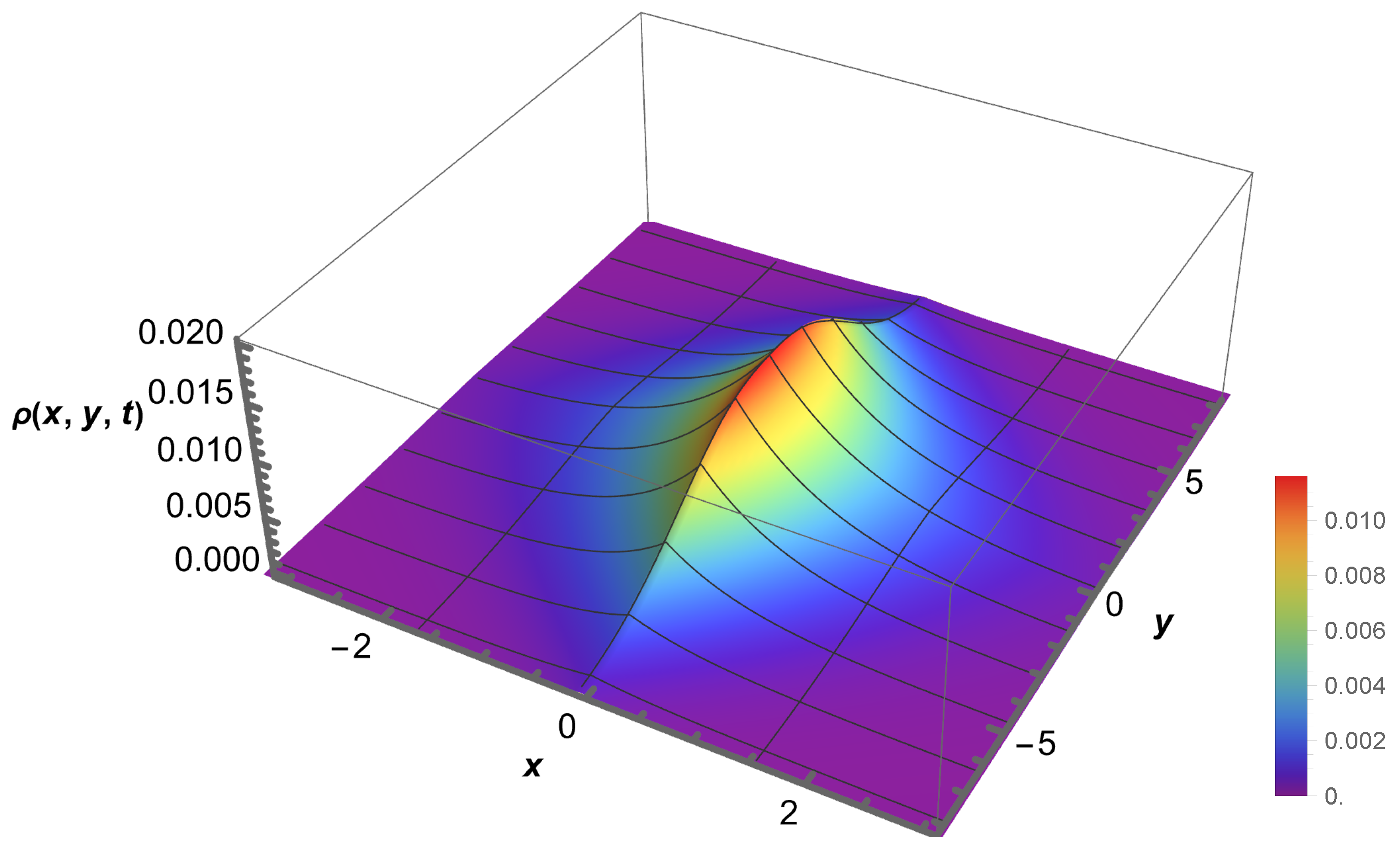
2. The Problem: Formal Investigation

Let us consider Equation (2) without stochastic resetting. In this case, Equation (2) can be written as follows:

$$\begin{array}{c}\hfill \begin{array}{c}\hfill {\displaystyle \frac{\partial }{\partial t}}\rho (\mathbf{r},t)={\mathcal{D}}_x\delta \left(y\right){\displaystyle \frac{{\partial }^2}{\partial x^2}}\rho (\mathbf{r},t)+{\mathcal{D}}_y{\displaystyle \frac{{\partial }^2}{\partial y^2}}\rho (\mathbf{r},t)-\mathcal{R}(\mathbf{r},t).\end{array}\end{array}$$

(4)

This equation combines a backbone structure and non-local linear terms, which can be related to fractional operators, reaction processes (reversible or irreversible), or trapping depending on the choice of the kernels. For example, the case $\mathfrak{K}\left(t\right)={\mathfrak{K}}_{\tau }{e}^{-t/\tau }$ can be related to the adsorption–desorption processes. Similar consideration can be performed when ${\mathfrak{K}}_{1,x}(x,t)\ne 0$ with ${\mathfrak{K}}_{2,x}(x,t)=0$; in this case, the particles are trapped in the x direction for some time, and after, they are released to diffuse. For the case, ${\mathfrak{K}}_{2,x}(x,t)\propto \delta \left(t\right)/{\left|x\right|}^{\mu -1}$ with $\mathfrak{K}\left(t\right)=0$ and ${\mathfrak{K}}_{1,x}\left(t\right)=0$, we can relate the non-local term to the fractional derivative in space. In particular, this choice for the nonlocal term leads us to obtain different diffusion regimes. It is worth noting that other fractional differential operators [56,57,58,59] can be considered depending on the choice of this kernel.

To obtain the solutions for the previous equation, we may use the integral transforms Laplace ($\mathcal{L}\{\rho (\mathbf{r},t);s\}=\widehat{\rho }(\mathbf{r},s))$ and Fourier (e.g., for the x variable, ${\mathfrak{F}}_x\{\rho (\mathbf{r},t);x\}=\tilde{\rho }(k_x,y,t)$), which allow us to obtain from Equation (4) the following equation:

$$\begin{array}{c}\hfill \begin{array}{c}\hfill s\widehat{\tilde{\rho }}(\mathbf{k},s)-\tilde{\phi }\left(\mathbf{k}\right)=-{\mathcal{D}}_x{k}_x^2\widehat{\tilde{\rho }}(k_x,y=0,s)-{\mathcal{D}}_y{k}_y^2\widehat{\tilde{\rho }}(\mathbf{k},s)-\widehat{\tilde{\mathcal{R}}}(\mathbf{k},s)\end{array}\end{array}$$

(5)

for the initial condition $\tilde{\rho }(\mathbf{k},0)=\tilde{\phi }\left(\mathbf{k}\right)$, with the non-local term given by

$$\begin{array}{c}\hfill \widehat{\tilde{\mathcal{R}}}(\mathbf{k},s)={\widehat{\tilde{\mathfrak{K}}}}_x(k_x,s)\widehat{\tilde{\rho }}(k_x,y=0,s)+\widehat{\mathfrak{K}}\left(s\right)\widehat{\rho }(0,0,s),\end{array}$$

(6)

where ${\widehat{\tilde{\mathfrak{K}}}}_x(k_x,s)={\widehat{\tilde{\mathfrak{K}}}}_{1,x}\left(s\right)+{\widehat{\tilde{\mathfrak{K}}}}_{2,x}(k_x,s)k_x^2$. By combining the previous equations, it is possible to show that

$$\begin{array}{c}\hfill \begin{array}{cc}\hfill \widehat{\tilde{\rho }}(\mathbf{k},s)& =\tilde{\phi }\left(\mathbf{k}\right){\widehat{\tilde{\mathcal{G}}}}_y(k_y,s)-\widehat{\mathfrak{K}}\left(s\right)\widehat{\rho }(0,0,s){\widehat{\tilde{\mathcal{G}}}}_y(k_y,s)\hfill \\ & -\left({\mathcal{D}}_x{k}_x^2+{\widehat{\tilde{\mathfrak{K}}}}_x(k_x,s)\right)\widehat{\tilde{\rho }}(k_x,y=0,s){\widehat{\tilde{\mathcal{G}}}}_y(k_y,s)\hfill \end{array}\end{array}$$

(7)

with

$$\begin{array}{c}\hfill {\widehat{\tilde{\mathcal{G}}}}_y(k_y,s)={\displaystyle \frac{1}{s+{\mathcal{D}}_y{k}_y^2}}.\end{array}$$

(8)

By performing some calculations, it is possible to show that

$$\begin{array}{c}\hfill \begin{array}{c}\hfill \widehat{\tilde{\rho }}(k_x,y=0,s)={\mathit{\int }}_{-\infty }^{\infty }d{y}^{\prime }\tilde{\phi }(k_x,y^{\prime }){\widehat{\mathcal{G}}}_y(y^{\prime },s)-\widehat{\mathfrak{K}}\left(s\right)\widehat{\rho }(0,0,s){\widehat{\tilde{\mathcal{G}}}}_x(k_x,s){\widehat{\mathcal{G}}}_y(0,s)\end{array}\end{array}$$

(9)

with

$$\begin{array}{c}\hfill {\widehat{\tilde{\mathcal{G}}}}_x(k_x,s)={\displaystyle \frac{1}{1+({\mathcal{D}}_x{k}_x^2+{\widehat{\tilde{\mathfrak{K}}}}_x(k_x,s)){\widehat{\mathcal{G}}}_y(0,s)}}\end{array}$$

(10)

and

$$\begin{array}{c}\hfill \widehat{\rho }(0,0,s)={\Phi }_1\left(s\right){\int }_{-\infty }^{\infty }d{x}^{\prime }{\int }_{-\infty }^{\infty }d{y}^{\prime }\phi (x^{\prime },y^{\prime }){\widehat{\mathcal{G}}}_y(y^{\prime },s){\widehat{\mathcal{G}}}_x(x^{\prime },s)\end{array}$$

(11)

with

$$\begin{array}{c}\hfill {\Phi }_1\left(s\right)={\displaystyle \frac{1}{1+\widehat{\mathfrak{K}}\left(s\right){\widehat{\mathcal{G}}}_y(0,s){\widehat{\mathcal{G}}}_x(0,s)}}.\end{array}$$

(12)

By using the previous results and performing some calculations, it is possible to show that

$$\begin{array}{c}\hfill \begin{array}{cc}\hfill & \widehat{\rho }(\mathbf{r},s)={\int }_{-\infty }^{\infty }d{y}^{\prime }\phi (x,y^{\prime })\left[{\widehat{\mathcal{G}}}_y(y-y^{\prime },s)-{\widehat{\mathcal{G}}}_y\left(\right|y|+|y^{\prime }|,s)\right]\hfill \\ & +{\int }_{-\infty }^{\infty }d{x}^{\prime }{\int }_{-\infty }^{\infty }d{y}^{\prime }\phi (x,y^{\prime })\left[{\widehat{\mathcal{G}}}_x(x-x^{\prime },s)-{\widehat{\mathcal{G}}}_x\left(\right|x|+|x^{\prime }|,s)\right]{\widehat{\mathcal{G}}}_y\left(\right|y|+|y^{\prime }|,s)\hfill \\ & +{\widehat{\Phi }}_1\left(s\right){\int }_{-\infty }^{\infty }d{x}^{\prime }{\int }_{-\infty }^{\infty }d{y}^{\prime }\phi (x,y^{\prime }){\widehat{\mathcal{G}}}_x\left(\right|x|+|x^{\prime }|,s){\widehat{\mathcal{G}}}_y\left(\right|y|+|y^{\prime }|,s)\hfill \end{array}\end{array}$$

(13)

and, consequently, after applying the inverse Laplace transform, we formally obtain the solution, which can be written as follows:

$$\begin{array}{c}\hfill \begin{array}{cc}\hfill & \rho (\mathbf{r},t)={\int }_{-\infty }^{\infty }d{y}^{\prime }\phi (x,y^{\prime })\left[{\mathcal{G}}_y(y-y^{\prime },t)-{\mathcal{G}}_y\left(\right|y|+|y^{\prime }|,t)\right]\hfill \\ & +{\int }_0^{t}d{t}^{\prime }{\int }_{-\infty }^{\infty }d{x}^{\prime }{\int }_{-\infty }^{\infty }d{y}^{\prime }\phi (x,y^{\prime })\left[{\mathcal{G}}_x(x-x^{\prime },t^{\prime })-{\mathcal{G}}_x\left(\right|x|+|x^{\prime }|,t^{\prime })\right]{\mathcal{G}}_y\left(\right|y|+|y^{\prime }|,t-t^{\prime })\hfill \\ & +{\int }_0^{t}d{t}^{\prime }{\mathrm{\Phi }}_1(t-t^{\prime }){\int }_0^{t^{\prime }}d{t}^{\prime \prime }{\int }_{-\infty }^{\infty }d{x}^{\prime }{\int }_{-\infty }^{\infty }d{y}^{\prime }\phi (x,y^{\prime }){\mathcal{G}}_x\left(\left|x\right|+|x^{\prime }|,t^{\prime \prime }\right){\mathcal{G}}_y\left(\left|y\right|+|y^{\prime }|,t^{\prime }-t^{\prime \prime }\right),\hfill \end{array}\end{array}$$

(14)

(see Figure 2). Note that the effect of the nonlocal term on the solution can be explicitly identified by the presence of the time-dependent function ${\mathrm{\Phi }}_1\left(t\right)$ and implicitly by the presence of ${\mathfrak{K}}_x(x,t)$ in Equation (10). This dependence on the nonlocal term directly influences the spreading of the system, as discussed below in terms of the mean square displacement.

The mean square displacement related to each direction can be obtained using the previous results to analyze the effect of the diffusion process’s non-local terms. For the x direction, we have that the mean square displacement is given by

$$\begin{array}{c}\hfill {\widehat{\sigma }}_x^2\left(s\right)={\displaystyle \frac{{\widehat{\Phi }}_1\left(s\right)({\mathcal{D}}_x+{\widehat{\overline{\mathfrak{K}}}}_{2,x}\left(s\right))}{s\sqrt{s{\mathcal{D}}_y}{(1+{\widehat{\mathfrak{K}}}_{1,x}\left(s\right)/\left(2\sqrt{s{\mathcal{D}}_y}\right))}^2}}\end{array}$$

(15)

for ${\widehat{\tilde{\mathfrak{K}}}}_x(k_x,s)={\widehat{\mathfrak{K}}}_{1,x}\left(s\right)+{\widehat{\overline{\mathfrak{K}}}}_{2,x}\left(s\right)k_x^2$, where only a time dependence for ${\mathfrak{K}}_{2,x}(x,t)$ is considered, i.e., ${\mathfrak{K}}_{2,x}(x,t)={\overline{\mathfrak{K}}}_{2,x}\left(t\right)\delta \left(x\right)$. For the y direction, we have that

$$\begin{array}{c}\hfill {\widehat{\sigma }}_y^2\left(s\right)={\displaystyle \frac{2{\mathcal{D}}_y\widehat{\Phi }\left(s\right)}{s^2{(1+{\widehat{\mathfrak{K}}}_{1,x}\left(s\right)/\left(2\sqrt{s{\mathcal{D}}_y}\right))}^2}}.\end{array}$$

(16)

Figure 3 and Figure 4 show the behavior of Equations (15) and (16) for a particular choice of the kernels. One of the main points observed in these figures is the presence of different diffusion regimes, where the last regime is slower than the first.

Now, let us incorporate stochastic resetting into the previous calculations. For this, we start by considering Equation (2) in the absence of the non-local terms, yielding

$$\begin{array}{c}\hfill \begin{array}{c}\hfill {\displaystyle \frac{\partial }{\partial t}}\rho (\mathbf{r},t)={\mathcal{D}}_x\delta \left(y\right){\displaystyle \frac{{\partial }^2}{\partial x^2}}\rho (\mathbf{r},t)+{\mathcal{D}}_y{\displaystyle \frac{{\partial }^2}{\partial y^2}}\rho (\mathbf{r},t)+\eta \left(\delta (\mathbf{r}-{\mathbf{r}}^{\prime })-\rho (\mathbf{r},t)\right).\end{array}\end{array}$$

(17)

It is worth mentioning that $\mathcal{S}\left(t\right)=1$ for this case, when the boundary conditions $\rho (\pm \infty ,y,t)=0$ and $\rho (x,\pm \infty ,t)=0$ are considered in absence of the nonlocal terms. Later on, we consider the boundary conditions $\rho (0,y,t)=\rho (\infty ,y,t)=0$ and $\rho (x,\pm \infty ,t)=0$, which will imply that $\mathcal{S}\left(t\right)\ne 1$. This feature is connected to the absorbent boundary condition present in $x=0$. The solution for Equation (17) can be found using the previous integral transform to simplify the previous equation. In particular, it is possible to show that

$$\begin{array}{cc}\hfill \widehat{\tilde{\rho }}(k_x,y,s)& ={\int }_{-\infty }^{\infty }d{y}^{\prime }\tilde{\phi }(k_x,y^{\prime }){\widehat{\mathcal{G}}}_{\eta ,y}(y-y^{\prime },s)-\eta e^{-k_x\overline{x}}{\widehat{\mathcal{G}}}_{\eta ,y}(y-y^{\prime },s)\end{array}$$

(18)

$$\begin{array}{cc}& -{\mathcal{D}}_x{k}_x^2\widehat{\tilde{\rho }}(k_x,y=0,s){\widehat{\mathcal{G}}}_{\eta ,y}(y,s)\end{array}$$

(19)

with

$$\begin{array}{c}\hfill {\widehat{\mathcal{G}}}_{\eta ,y}(y,s)={\displaystyle \frac{e^{-\sqrt{s+\eta }\frac{\left|y\right|}{{\sqrt{\mathcal{D}}}_y}}}{2\sqrt{(s+\eta ){\mathcal{D}}_y}}}.\end{array}$$

(20)

From these results, we can show that

$$\begin{array}{c}\hfill \begin{array}{cc}\hfill & \widehat{\rho }(\mathbf{r},s)={\int }_{-\infty }^{\infty }d{y}^{\prime }\phi (x,y^{\prime })\left[{\widehat{\mathcal{G}}}_{\eta ,y}(y-y^{\prime },s)-{\widehat{\mathcal{G}}}_{\eta ,y}\left(\right|y|+|y^{\prime }|,s)\right]\hfill \\ & +{\displaystyle \frac{\eta }{s}}{\widehat{\mathcal{G}}}_{\eta ,y}\left(\right|y|+|\overline{y}|,s){\widehat{\mathcal{G}}}_{\eta ,x}(x-\overline{x},s)+\eta \delta (x-\overline{x})\left[{\widehat{\mathcal{G}}}_{\eta ,y}(y-\overline{y},s)-{\widehat{\mathcal{G}}}_{\eta ,y}\left(\right|y|+|\overline{y}|,s)\right]\hfill \\ & +{\int }_{-\infty }^{\infty }d{x}^{\prime }{\int }_{-\infty }^{\infty }d{y}^{\prime }\phi (x^{\prime },y^{\prime }){\widehat{\mathcal{G}}}_{\eta ,y}\left(\right|y|+|y^{\prime }|,s){\widehat{\mathcal{G}}}_{\eta ,x}(x-x^{\prime },s),\hfill \end{array}\end{array}$$

(21)

with

$$\begin{array}{c}\hfill {\widehat{\mathcal{G}}}_{\eta ,x}(k_x,s)={\displaystyle \frac{e^{-\frac{\left|x\right|}{\sqrt{{\mathcal{D}}_x{\widehat{\mathcal{G}}}_{\eta ,y}(0,s)}}}}{2\sqrt{{\mathcal{D}}_x{\widehat{\mathcal{G}}}_{\eta ,y}(0,s)}}}.\end{array}$$

(22)

Equation (21) has additional terms related to the stochastic resetting, which are not present in Equation (13). The inverse Laplace transform of Equation (21) can be written as follows:

$$\begin{array}{c}\hfill \begin{array}{cc}\hfill & \rho (\mathbf{r},t)={\int }_{-\infty }^{\infty }d{y}^{\prime }\phi (x,y^{\prime })\left[{\mathcal{G}}_{\eta ,y}(y-y^{\prime },t)-{\mathcal{G}}_{\eta ,y}\left(\right|y|+|y^{\prime }|,t)\right]\hfill \\ & +{\int }_0^{t}d{t}^{\prime }{\int }_0^{t^{\prime }}d{t}^{\prime \prime }\eta {\mathcal{G}}_{\eta ,y}\left(\right|y|+|\overline{y}|,t^{\prime }-t^{\prime \prime }){\mathcal{G}}_{\eta ,x}(x-\overline{x},t^{\prime \prime })\hfill \\ & +\eta \delta (x-\overline{x})\left[{\mathcal{G}}_{\eta ,y}(y-\overline{y},t)-{\mathcal{G}}_{\eta ,y}\left(\right|y|+|\overline{y}|,t)\right]\hfill \\ & +{\int }_0^{t}d{t}^{\prime }{\int }_{-\infty }^{\infty }d{x}^{\prime }{\int }_{-\infty }^{\infty }d{y}^{\prime }\phi (x^{\prime },y^{\prime }){\mathcal{G}}_{\eta ,y}\left(\right|y|+|y^{\prime }|,t-t^{\prime }){\mathcal{G}}_{\eta ,x}(x-x^{\prime },t^{\prime }).\hfill \end{array}\end{array}$$

(23)

Now, we consider the previous scenario with the boundary condition $\rho (0,y,t)=0$, which implies an absorbent surface in $x=0$, and analyze the mean first passage time in this scenario. For this, we consider the previous equation as follows:

$$\begin{array}{c}\hfill \begin{array}{c}\hfill {\displaystyle \frac{\partial }{\partial t}}\rho (\mathbf{r},t)={\mathcal{D}}_x\delta \left(y\right){\displaystyle \frac{{\partial }^2}{\partial x^2}}\rho (\mathbf{r},t)+{\mathcal{D}}_y{\displaystyle \frac{{\partial }^2}{\partial y^2}}\rho (\mathbf{r},t)+\eta \left(\mathcal{S}\left(t\right)\delta (\mathbf{r}-{\mathbf{r}}^{\prime })-\rho (\mathbf{r},t)\right).\end{array}\end{array}$$

(24)

Note that the presence of the survival probability, i.e., $S\left(t\right)$, in Equation (24) is connected with the feature that the particles of the system are not constant in time, which is different from the previous case due to the absorbent surface. We use the previous procedure based on integral transforms to solve Equation (24). For the x variable, we consider the sine Fourier transform, yielding

$$\begin{array}{c}\hfill \begin{array}{cc}& \widehat{\rho }(\mathbf{r},s)={\int }_{-\infty }^{\infty }d{y}^{\prime }\phi (x,y^{\prime })\left[{\widehat{\mathcal{G}}}_{\eta ,y}(y-y^{\prime },s)-{\widehat{\mathcal{G}}}_{\eta ,y}\left(\right|y|+|y^{\prime }|,s)\right]\hfill \\ & +\eta \widehat{\mathcal{S}}\left(s\right){\widehat{\mathcal{G}}}_{\eta ,y}\left(\right|y|+|\overline{y}|,s){\widehat{\mathcal{G}}}_{\eta ,x}^{\left(1\right)}(x,\overline{x},s)\hfill \\ & +\eta \delta (x-\overline{x})\widehat{\mathcal{S}}\left(s\right)\left[{\widehat{\mathcal{G}}}_{\eta ,y}(y-\overline{y},s)-{\widehat{\mathcal{G}}}_{\eta ,y}\left(\right|y|+|\overline{y}|,s)\right]\hfill \\ & +{\int }_{-\infty }^{\infty }d{x}^{\prime }{\int }_{-\infty }^{\infty }d{y}^{\prime }\phi (x^{\prime },y^{\prime }){\widehat{\mathcal{G}}}_{\eta ,y}\left(\right|y|+|y^{\prime }|,s){\widehat{\mathcal{G}}}_{\eta ,x}^{\left(1\right)}(x,x^{\prime },s),\hfill \end{array}\end{array}$$

(25)

with

$$\begin{array}{c}\hfill {\widehat{\mathcal{G}}}_{\eta ,x}^{\left(1\right)}(x,x^{\prime },s)={\displaystyle \frac{1}{2\sqrt{{\mathcal{D}}_x{\widehat{\mathcal{G}}}_y(0,s)}}}\left(e^{-{\displaystyle \frac{|x-x^{\prime }|}{\sqrt{{\mathcal{D}}_x{\widehat{\mathcal{G}}}_y(0,s)}}}}-e^{-{\displaystyle \frac{|x+x^{\prime }|}{\sqrt{{\mathcal{D}}_x{\widehat{\mathcal{G}}}_y(0,s)}}}}\right).\end{array}$$

(26)

From the Equation (25) with $\overline{y}=0$ and $\phi (x,y)=\delta (x-x^{\prime })\delta \left(y\right)$, we obtain that survival probability is given by

$$\begin{array}{c}\hfill \widehat{\mathcal{S}}\left(s\right)=[1-e^{-\frac{|x^{\prime }|}{\sqrt{{\mathcal{D}}_x{\widehat{\mathcal{G}}}_y(0,s)}}}]/\left[s+\eta e^{-\frac{|\overline{x}|}{\sqrt{{\mathcal{D}}_x{\widehat{\mathcal{G}}}_y(0,s)}}}\right].\end{array}$$

(27)

The mean first passage time can be obtained from the previous equation and results in

$$\begin{array}{c}\hfill T(x^{\prime },\overline{x})={\displaystyle \frac{1}{\eta }}{e}^{\sqrt{{\displaystyle \frac{2\sqrt{\eta {\mathcal{D}}_y}}{{\mathcal{D}}_x}}}\left|\overline{x}\right|}\left(1-e^{\sqrt{{\displaystyle \frac{2\sqrt{\eta {\mathcal{D}}_y}}{{\mathcal{D}}_x}}}\left|x^{\prime }\right|}\right).\end{array}$$

(28)

(see Figure 5). By performing some calculations for usual diffusion, it is possible to obtain the expression for the mean first passage time. It is given by

$$\begin{array}{c}\hfill T(x^{\prime },\overline{x})={\displaystyle \frac{1}{\eta }}{e}^{\sqrt{{\displaystyle \frac{\eta }{{\mathcal{D}}_x}}}\left|\overline{x}\right|}\left(1-e^{\sqrt{{\displaystyle \frac{\eta }{{\mathcal{D}}_x}}}\left|x^{\prime }\right|}\right),\end{array}$$

(29)

which is different from Equation (28). In the limit of $\eta \to 0$, it is possible to verify that $T(x^{\prime },\overline{x})\sim 1/{\eta }^{3/4}$ for the comb model and $T(x^{\prime },\overline{x})\sim 1/{\eta }^{1/2}$ for the standard case. This difference manifested for the mean first passage time can be related to the geometric structure present in the comb model, which restricts the diffusion process.

After the previous analysis, we consider the stochastic reset combined with the non-local terms by considering the case ${\widehat{\tilde{\mathfrak{K}}}}_x(k_x,s)={\widehat{\mathfrak{K}}}_{2,x}\left(s\right)k_x^2$ with $\widehat{\tilde{\mathfrak{K}}}\left(s\right)$ arbitrary. The solution can be found, and it is given by

$$\begin{array}{c}\hfill \begin{array}{cc}& \widehat{\rho }(\mathbf{r},s)={\int }_{-\infty }^{\infty }d{y}^{\prime }\phi (x,y^{\prime })\left[{\widehat{\mathcal{G}}}_{\eta ,y}(y-y^{\prime },s)-{\widehat{\mathcal{G}}}_{\eta ,y}\left(\right|y|+|y^{\prime }|,s)\right]\hfill \\ & +{\displaystyle \frac{\eta }{s}}{\widehat{\mathcal{G}}}_{\eta ,y}\left(\right|y|+|\overline{y}|,s){\widehat{\mathcal{G}}}_{\eta ,x}^{\left(2\right)}(x-\overline{x},s)+\eta \delta (x-\overline{x})\left[{\widehat{\mathcal{G}}}_{\eta ,y}(y-\overline{y},s)-{\widehat{\mathcal{G}}}_{\eta ,y}\left(\right|y|+|\overline{y}|,s)\right]\widehat{\mathcal{S}}\left(s\right)\hfill \\ & +{\int }_{-\infty }^{\infty }d{x}^{\prime }{\int }_{-\infty }^{\infty }d{y}^{\prime }\phi (x^{\prime },y^{\prime }){\widehat{\mathcal{G}}}_{\eta ,y}\left(\right|y|+|y^{\prime }|,s){\widehat{\mathcal{G}}}_{\eta ,x}^{\left(2\right)}(x-x^{\prime },s)\hfill \\ & +\widehat{\mathfrak{K}}\left(s\right)\left[{\widehat{\mathcal{G}}}_{\eta ,y}(y,s){\widehat{\mathcal{G}}}_{\eta ,x}^{\left(2\right)}(x,s)-{\displaystyle \frac{\eta }{s}}{\widehat{\mathcal{G}}}_{\eta ,x}^{\left(2\right)}(x-\overline{x},s){\widehat{\mathcal{G}}}_{\eta ,y}\left(\right|y|+|\overline{y}|,s)\right]\widehat{\rho }(0,0,s),\hfill \end{array}\end{array}$$

(30)

where $\widehat{\mathcal{S}}\left(s\right)=(1-\widehat{\mathfrak{K}}\left(s\right)\widehat{\rho }(0,0,s))/s$

$$\begin{array}{c}\hfill \widehat{\rho }(0,0,s)={\Phi }_{2,\eta }\left(s\right)\left[{\int }_{-\infty }^{\infty }d{x}^{\prime }{\int }_{-\infty }^{\infty }d{y}^{\prime }\phi (x^{\prime },y^{\prime }){\mathcal{G}}_{\eta ,y}(y^{\prime },s){\mathcal{G}}_{\eta ,x}^{\left(2\right)}(x^{\prime },s)+{\displaystyle \frac{\eta }{s}}{\mathcal{G}}_{\eta ,y}(\overline{y},s){\mathcal{G}}_{\eta ,x}^{\left(2\right)}(\overline{x},s)\right],\end{array}$$

(31)

$$\begin{array}{c}\hfill {\widehat{\mathcal{G}}}_{\eta ,x}^{\left(2\right)}(k_x,s)={\displaystyle \frac{e^{-\frac{\left|x\right|}{\sqrt{({\mathcal{D}}_x+{\widehat{\mathfrak{K}}}_{2,x}\left(s\right)){\widehat{\mathcal{G}}}_{\eta ,y}(0,s)}}}}{2\sqrt{({\mathcal{D}}_x+{\widehat{\mathfrak{K}}}_{2,x}\left(s\right)){\widehat{\mathcal{G}}}_{\eta ,y}(0,s)}}},\end{array}$$

(32)

and

$$\begin{array}{c}\hfill {\Phi }_{2,\eta }\left(s\right)={\left[1+\widehat{\mathfrak{K}}\left(s\right)\left[{\widehat{\mathcal{G}}}_{\eta ,y}(0,s){\widehat{\mathcal{G}}}_{\eta ,x}^{\left(2\right)}(0,s)+\left(\eta /s\right){\widehat{\mathcal{G}}}_{\eta ,y}(\overline{y},s){\widehat{\mathcal{G}}}_{\eta ,x}^{\left(2\right)}(\overline{x},s)\right]\right]}^{-1}.\end{array}$$

(33)

Note that Equation (30) has additional contributions related to the nonlocal terms, in contrast with Equation (21), which has only the influence of the stochastic resetting. For the particular case $\overline{x}=0$ and $\overline{y}=0$, we obtain, in the Laplace domain, that

$$\begin{array}{c}\hfill \begin{array}{cc}\hfill & \widehat{\rho }(\mathbf{r},s)={\int }_{-\infty }^{\infty }d{y}^{\prime }\phi (x,y^{\prime })\left[{\mathcal{G}}_{\eta ,y}(y-y^{\prime },s)-{\mathcal{G}}_{\eta ,y}\left(\right|y|+|y^{\prime }|,s)\right]+{\displaystyle \frac{\eta }{s}}{\Phi }_{2,\eta }\left(s\right){\mathcal{G}}_{\eta ,x}^{\left(2\right)}(x,s){\mathcal{G}}_{\eta ,y}(y,s)\hfill \\ & +{\int }_{-\infty }^{\infty }d{x}^{\prime }{\int }_{-\infty }^{\infty }d{y}^{\prime }\phi (x^{\prime },y^{\prime })\left[{\mathcal{G}}_{\eta ,x}^{\left(2\right)}(x-x^{\prime },s)-{\mathcal{G}}_{\eta ,x}^{\left(2\right)}\left(\right|x|+|x^{\prime }|,s)\right]{\mathcal{G}}_{\eta ,y}\left(\right|y|+|y^{\prime }|,s)\hfill \\ & +{\Phi }_{2,\eta }\left(s\right){\int }_{-\infty }^{\infty }d{x}^{\prime }{\int }_{-\infty }^{\infty }d{y}^{\prime }\phi (x^{\prime },y^{\prime }){\mathcal{G}}_{\eta ,x}^{\left(2\right)}\left(\right|x|+|x^{\prime }|,s){\mathcal{G}}_{\eta ,y}\left(\right|y|+|y^{\prime }|,s)],\hfill \end{array}\end{array}$$

(34)

(see Figure 6).

Figure 7 and Figure 8 show the behavior of the mean square displacement obtained from Equation (34). It is possible to observe that the stochastic resetting changes the last diffusion regime.

Let us consider the case ${\widehat{\tilde{\mathfrak{K}}}}_x(k_x,s)={\widehat{\mathfrak{K}}}_{1,x}\left(s\right)+{\widehat{\mathfrak{K}}}_{2,x}\left(s\right)k_x^2$ for the non-local term in the backbone structure. In this case, by performing some calculations, it is possible to show, in the Laplace domain, that

$$\begin{array}{c}\hfill \begin{array}{cc}& \widehat{\rho }(\mathbf{r},s)={\int }_{-\infty }^{\infty }d{y}^{\prime }\phi (x,y^{\prime })\left[{\widehat{\mathcal{G}}}_{\eta ,y}(y-y^{\prime },s)-{\widehat{\mathcal{G}}}_{\eta ,y}\left(\right|y|+|y^{\prime }|,s)\right]\hfill \\ & +{\widehat{\Phi }}_{3,\eta }\left(s\right)\mathcal{S}\left(s\right){\widehat{\mathcal{G}}}_{\eta ,y}\left(\right|y|+|\overline{y}|,s){\widehat{\mathcal{G}}}_{\eta ,x}^{\left(3\right)}\left(\right|x|+|\overline{x}|,s)\hfill \\ & +\eta \widehat{\mathcal{S}}\left(s\right){\widehat{\mathcal{G}}}_{\eta ,y}\left(\right|y|+|\overline{y}|,s)\left[{\widehat{\mathcal{G}}}_{\eta ,x}^{\left(3\right)}(x-\overline{x},s)-{\widehat{\mathcal{G}}}_{\eta ,x}^{\left(3\right)}\left(\right|x|+|\overline{x}|,s)\right]\hfill \\ & +\eta \delta (x-\overline{x})\left[{\widehat{\mathcal{G}}}_{\eta ,y}(y-\overline{y},s)-{\widehat{\mathcal{G}}}_{\eta ,y}\left(\right|y|+|\overline{y}|,s)\right]\widehat{\mathcal{S}}\left(s\right)\hfill \\ & +{\int }_{-\infty }^{\infty }d{x}^{\prime }{\int }_{-\infty }^{\infty }d{y}^{\prime }\phi (x^{\prime },y^{\prime }){\widehat{\mathcal{G}}}_{\eta ,y}\left(\right|y|+|y^{\prime }|,s)\left[{\widehat{\mathcal{G}}}_{\eta ,x}^{\left(3\right)}(x-x^{\prime },s)-{\widehat{\mathcal{G}}}_{\eta ,x}^{\left(3\right)}\left(\right|x|+|x^{\prime }|,s)\right]\hfill \\ & +{\widehat{\Phi }}_{3,\eta }\left(s\right){\int }_{-\infty }^{\infty }d{x}^{\prime }{\int }_{-\infty }^{\infty }d{y}^{\prime }\phi (x^{\prime },y^{\prime }){\widehat{\mathcal{G}}}_{\eta ,y}\left(\right|y|+|y^{\prime }|,s){\widehat{\mathcal{G}}}_{\eta ,x}^{\left(3\right)}(x-x^{\prime },s),\hfill \end{array}\end{array}$$

(35)

where

$$\begin{array}{c}\hfill {\widehat{\mathcal{G}}}_{\eta ,x}^{\left(3\right)}(x,s)={\displaystyle \frac{e^{-\sqrt{\frac{1+{\widehat{\mathfrak{K}}}_{1,x}\left(s\right){\widehat{\mathcal{G}}}_{\eta ,y}(0,s)}{({\mathcal{D}}_x+{\widehat{\mathfrak{K}}}_{2,x}\left(s\right)){\widehat{\mathcal{G}}}_{\eta ,y}(0,s)}}\left|x\right|}}{2\sqrt{(1+{\widehat{\mathfrak{K}}}_{1,x}\left(s\right){\widehat{\mathcal{G}}}_{\eta ,y}(0,s))({\mathcal{D}}_x+{\widehat{\mathfrak{K}}}_{2,x}\left(s\right)){\widehat{\mathcal{G}}}_{\eta ,y}(0,s)}}},\end{array}$$

(36)

with ${\Phi }_{3,\eta }\left(s\right)=1/\left[1+\widehat{\mathfrak{K}}\left(s\right){\widehat{\mathcal{G}}}_{\eta ,y}(0,s){\widehat{\mathcal{G}}}_{\eta ,x}^{\left(3\right)}(0,s)\right]$,

$$\begin{array}{c}\hfill \begin{array}{cc}\hfill \widehat{\rho }(0,0,s)& ={\Phi }_{3,\eta }\left(s\right){\int }_{-\infty }^{\infty }d{x}^{\prime }{\int }_{-\infty }^{\infty }d{y}^{\prime }\phi (x^{\prime },y^{\prime }){\mathcal{G}}_{\eta ,y}(y^{\prime },s){\mathcal{G}}_{\eta ,x}^{\left(3\right)}(x^{\prime },s)\hfill \\ & +\eta {\Phi }_{3,\eta }\left(s\right)\widehat{S}\left(s\right){\widehat{\mathcal{G}}}_{\eta ,y}(\overline{y},s){\mathcal{G}}_{\eta ,x}^{\left(3\right)}(\overline{x},s),\hfill \end{array}\end{array}$$

(37)

$$\begin{array}{c}\hfill \begin{array}{cc}\hfill \widehat{\mathcal{S}}\left(s\right)& =\widehat{{\rm Y}}\left(s\right){\int }_{-\infty }^{\infty }d{x}^{\prime }{\int }_{-\infty }^{\infty }d{y}^{\prime }\phi (x^{\prime },y^{\prime })\left[1-{\widehat{\mathfrak{K}}}_{1,x}\left(s\right){\widehat{\mathcal{G}}}_{\eta ,y}(y^{\prime },s)\right]\hfill \\ & -\widehat{{\rm Y}}\left(s\right)\widehat{\mathfrak{K}}\left(s\right)\left[1-{\widehat{\mathfrak{K}}}_{1,x}\left(s\right){\widehat{\mathcal{G}}}_{\eta ,y}(0,s){\widehat{\tilde{\mathcal{G}}}}_{\eta ,x}^{\left(3\right)}(0,s)\right]\widehat{\rho }(0,0,s),\hfill \end{array}\end{array}$$

(38)

and $\widehat{{\rm Y}}\left(s\right)=1/\left[s+\eta {\widehat{\mathfrak{K}}}_{1,x}\left(s\right){\widehat{\mathcal{G}}}_{\eta ,y}(\overline{y},s){\widehat{\mathcal{G}}}_{\eta ,x}^{\left(3\right)}(\overline{x},s)\right]$. Note that Equations (35) to (38) consider an arbitrary dependence on the kernels, and the inverse of the Laplace transform depends on the choice performed for each kernel, and they are an extension of the previous ones. Figure 9 and Figure 10 show the behavior of Equation (35) for $\eta =0.1$ and $\eta =1$ to evidence the effect of the stochastic resetting on the distribution.

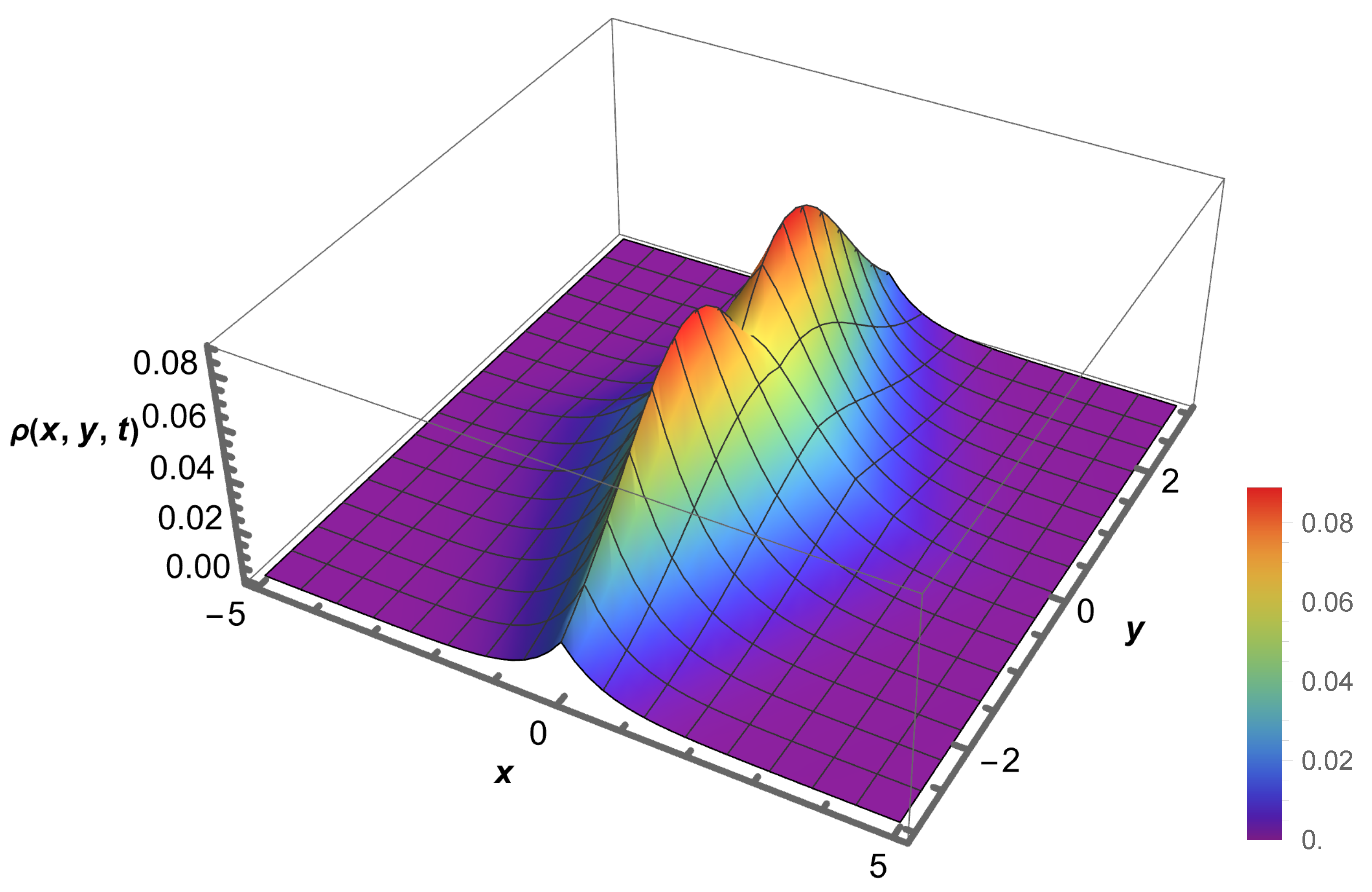
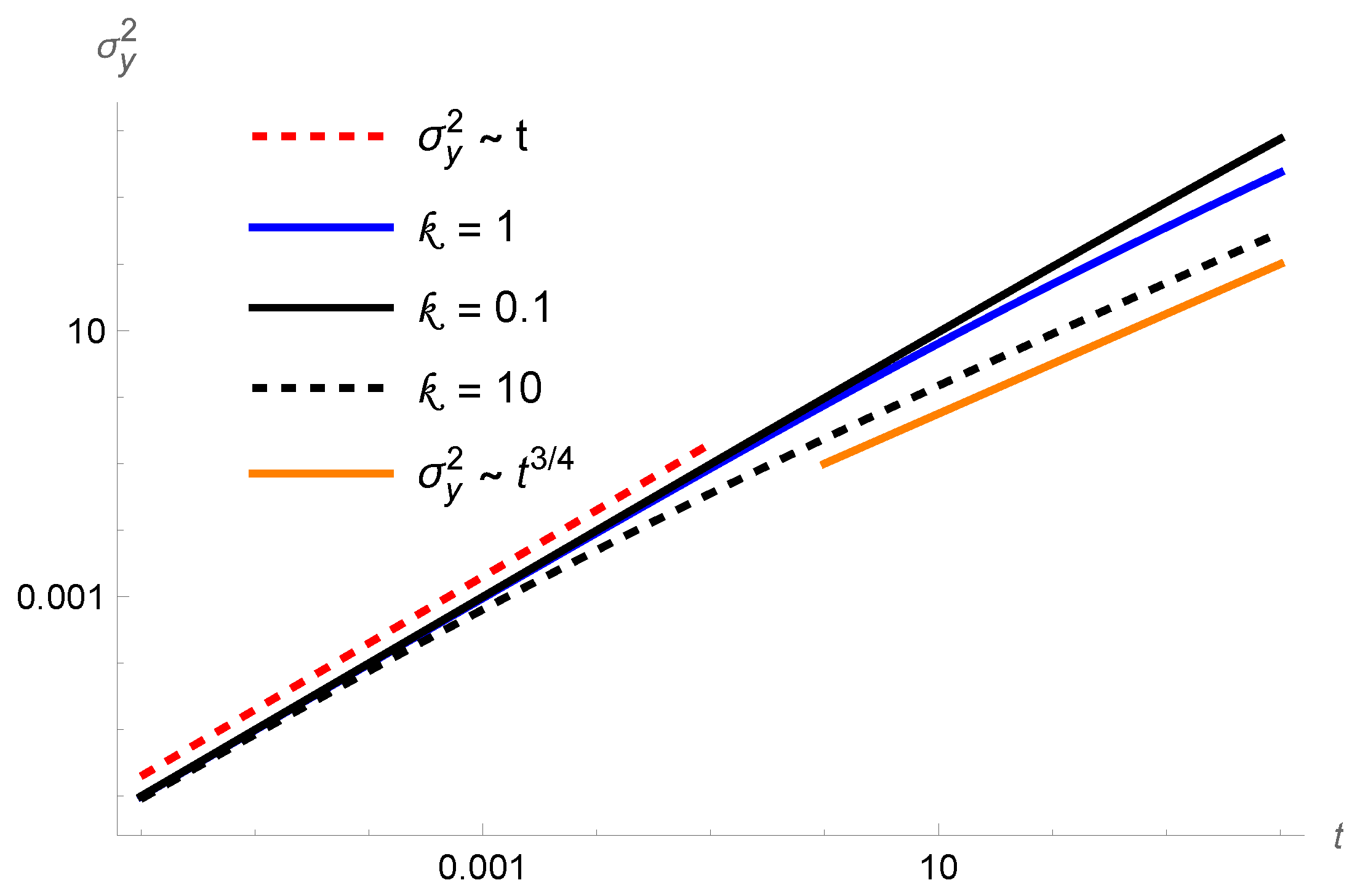
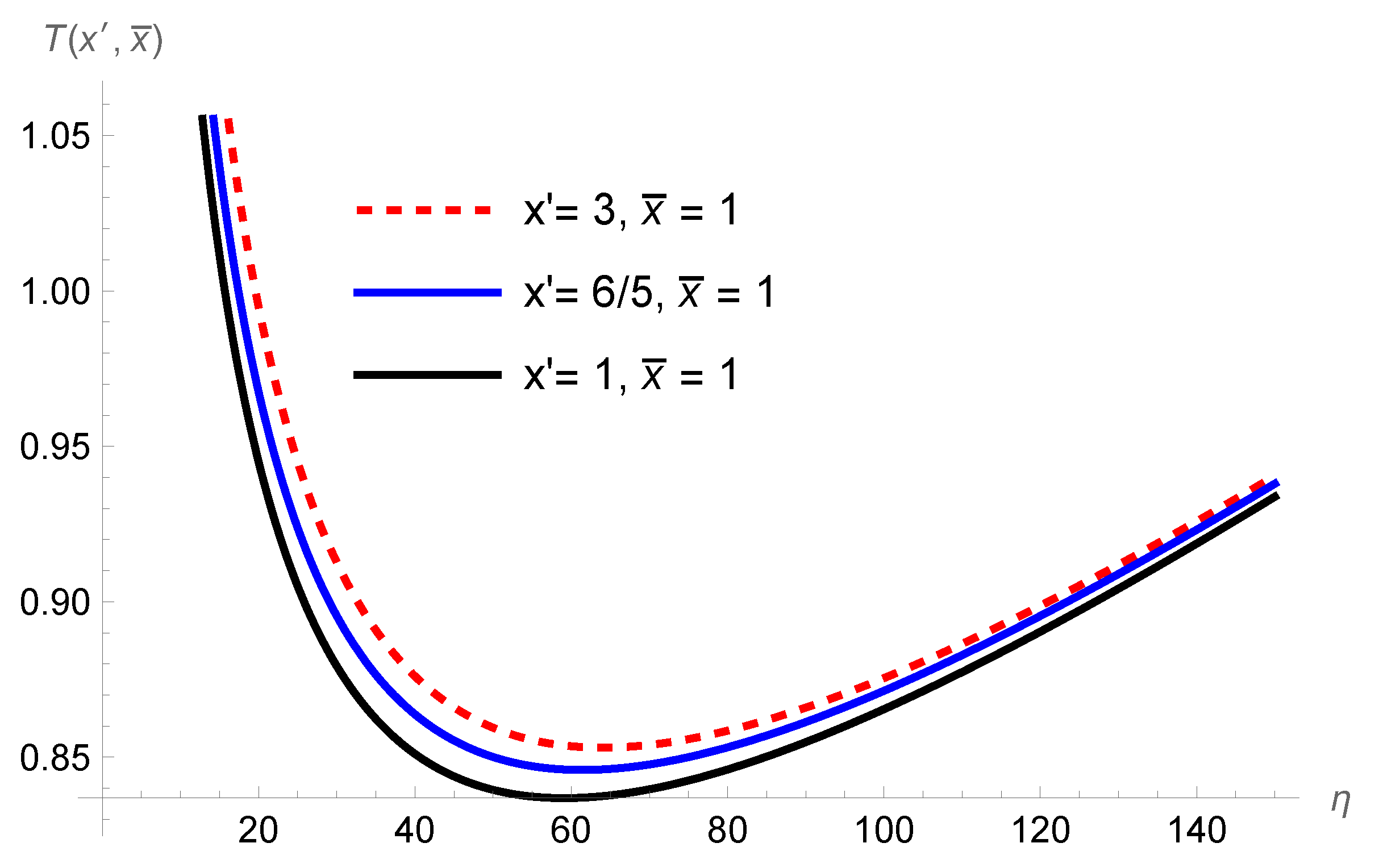
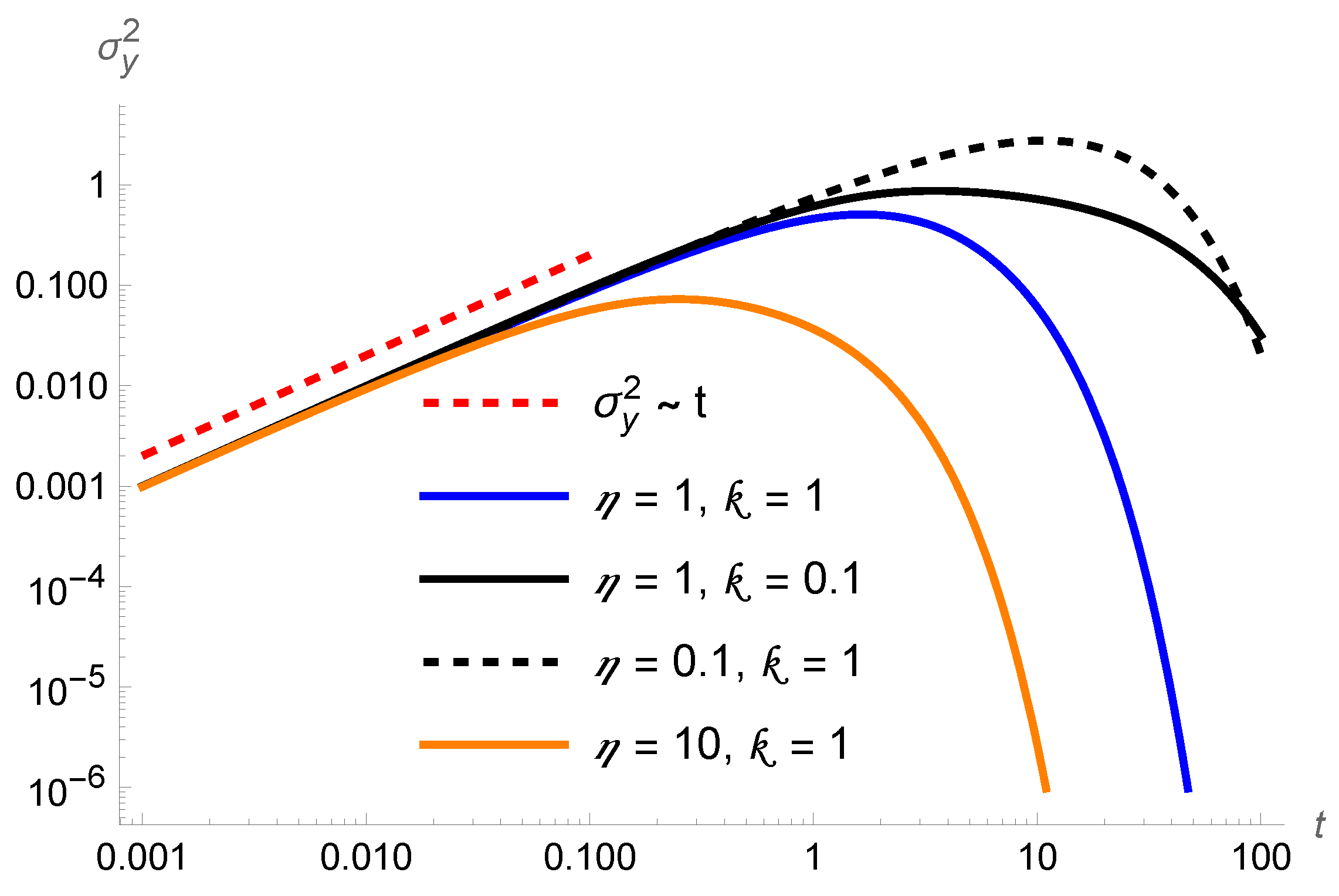
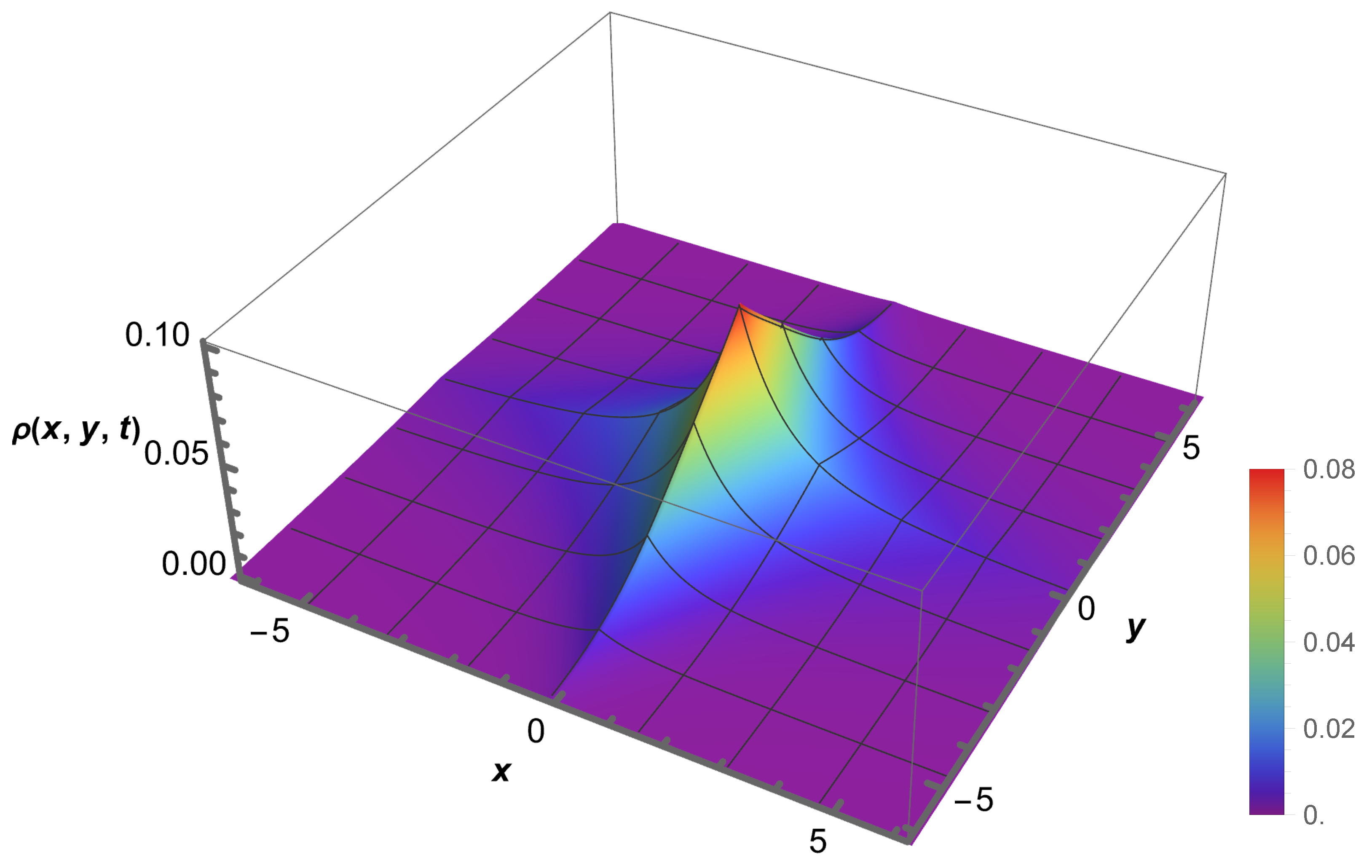
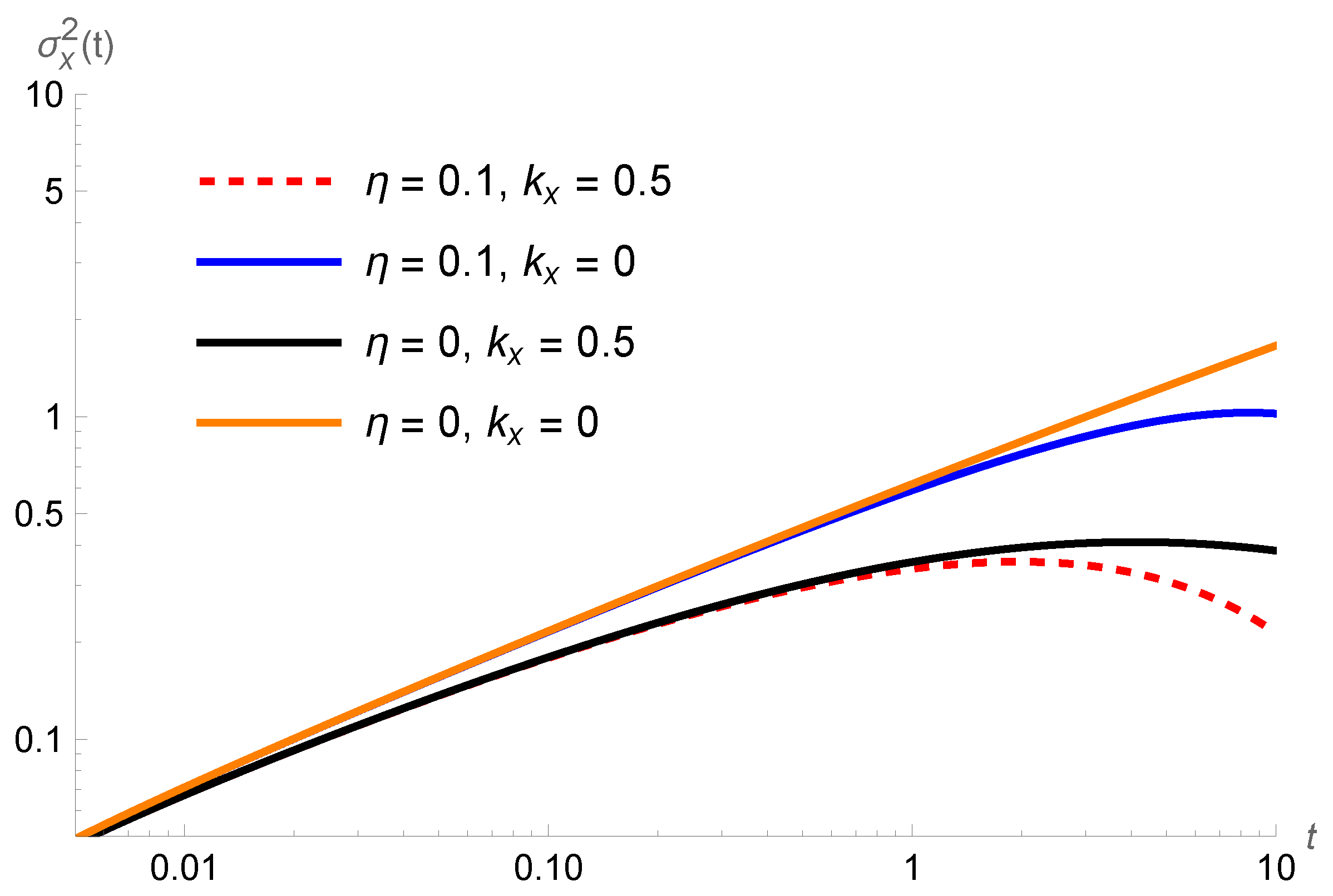
3. The Problem: Numerical Investigation

Now, we consider a numerical calculation to solve the previous equation. We solve numerically using the explicit method. First, we consider the following equation, i.e.,

$$\begin{array}{c}\hfill \begin{array}{cc}\hfill {\displaystyle \frac{\partial }{\partial t}}\rho (\mathbf{r},t)={\mathcal{D}}_x\delta \left(y\right){\displaystyle \frac{{\partial }^2}{\partial x^2}}\rho (\mathbf{r},t)& +{\mathcal{D}}_y{\displaystyle \frac{{\partial }^2}{\partial y^2}}\rho (\mathbf{r},t)-\mathcal{R}(\mathbf{r},t)+\eta \left(\mathcal{S}\left(t\right)\delta \left(\mathbf{r}\right)-\rho (\mathbf{r},t)\right),\hfill \end{array}\end{array}$$

(39)

with

$$\begin{array}{c}\hfill \begin{array}{cc}\hfill \mathcal{R}(\mathbf{r},t)& =\delta \left(y\right){\mathfrak{K}}_x\rho (\mathbf{r},t)+\delta \left(x\right)\delta \left(y\right)\mathfrak{K}\rho (\mathbf{r},t).\hfill \end{array}\end{array}$$

(40)

The previous equation corresponds to Equation (3) with ${\mathfrak{K}}_{1,x}\left(t\right)=\delta \left(t\right){\mathfrak{K}}_x$, ${\mathfrak{K}}_{2,x}(x,t)=0$, and $\mathfrak{K}\left(t\right)=\delta \left(t\right)\mathfrak{K}$. The reaction term $\mathcal{R}(\mathbf{r},t)$ with these choices accounts for localized losses, while $\eta$ governs the stochastic resetting term. To solve this equation numerically, we perform a discretization in space and time using a finite difference scheme. Let i and j represent the discrete spatial indices in the x and y directions, respectively, with a spatial step size $h_x$. Similarly, n represents the discrete time index with a time step size $h_t$. The survival probability or area at time $n{h}_t$ is denoted by $S\left(n\right)$. The explicit discretization of Equation (42) is given by

$$\begin{array}{c}\hfill \begin{array}{cc}\hfill {\rho }_{[i,j,n+1]}& ={\rho }_{[i,j,n]}+(j=0)\left(h_t/h_x^3\right){\mathcal{D}}_x\left({\rho }_{[i-1,j,n]}-2{\rho }_{[i,j,n]}+{\rho }_{[i+1,j,n]}\right)\hfill \\ & +\left(h_t/h_x^2\right){\mathcal{D}}_y\left({\rho }_{[i,j-1,n]}-2{\rho }_{[i,j,n]}+{\rho }_{[i,j+1,n]}\right)-(i=0)(j=0)\left(h_t/h_x^2\right)\mathfrak{K}{\rho }_{[i,j,n]}\hfill \\ & -(j=0)\left(h_t/h_x\right){\mathfrak{K}}_x{\rho }_{[i,j,n]}+\eta h_t\left(\left((i=0)(j=0)/h_x^2\right)S\left(n\right)-{\rho }_{[i,j,n]}\right)\hfill \end{array}\end{array}$$

(41)

(for more details see the Appendix A). Figure 11, Figure 12 and Figure 13 illustrate the behavior of the system for the distribution and the mean square displacement when Equation (41) is considered.

Let us consider a spatial dependence for the non-local term in the backbone structure, i.e., we consider Equation (3), given by

$$\begin{array}{c}\hfill \begin{array}{c}\hfill \mathcal{R}(\mathbf{r},t)=\delta \left(x\right)\delta \left(y\right)\mathfrak{K}\rho (\mathbf{r},t)-\delta \left(y\right){\mathfrak{K}}_x{\int }_{-\infty }^{\infty }d{x}^{\prime }{e}^{-\alpha |x-x^{\prime }|}{\displaystyle \frac{{\partial }^2}{\partial x^{\prime 2}}}\rho (x^{\prime },y,t).\end{array}\end{array}$$

(42)

Note that the previous equation results from Equation (3) with ${\mathfrak{K}}_{1,x}\left(t\right)=0$, ${\mathfrak{K}}_{2,x}(x,t)={\mathfrak{K}}_x{e}^{-\alpha \left|x\right|}\delta \left(t\right)$, and $\mathfrak{K}\left(t\right)=\delta \left(t\right)\mathfrak{K}$. This choice for the kernels differs from the ones in the previous section, i.e., the memory effect is connected with a kernel with a spatial dependence. The discretization of the term with the kernel with a spatial dependence can be written as

$$\begin{array}{c}\hfill \begin{array}{cc}\hfill {\int }_{-\infty }^{\infty }d{x}^{\prime }{e}^{-\alpha |x-x^{\prime }|}& {\displaystyle \frac{{\partial }^2}{\partial x^{\prime 2}}}\rho (x^{\prime },y,t^{\prime })=F(i,j,n)\hfill \\ & ={\displaystyle \frac{1}{h_x^2\alpha }}\sum _{k=-L}^{k=i-1}\left({\rho }_{[k+1,j,n]}-2{\rho }_{[k,j,n]}+{\rho }_{[k-1,j,n]}\right)\left(e^{h_x\alpha (-i+k)}(-1+e^{h_x\alpha })\right)\hfill \\ & +{\displaystyle \frac{1}{h_x^2\alpha }}\sum _{k=i}^{k=L-1}\left({\rho }_{[k+1,j,n]}-2{\rho }_{[k,j,n]}+{\rho }_{[k-1,j,n]}\right)\left(e^{h_x\alpha (i-k-1)}(-1+e^{h_x\alpha })\right),\hfill \end{array}\end{array}$$

(43)

which yields

$$\begin{array}{c}\hfill \begin{array}{cc}\hfill {\rho }_{[i,j,n+1]}& ={\rho }_{[i,j,n]}+(j=0)\left(h_t/h_x^3\right){\mathcal{D}}_x\left({\rho }_{[i-1,j,n]}-2{\rho }_{[i,j,n]}+{\rho }_{[i+1,j,n]}\right)\hfill \\ & +\left(h_t/h_x^2\right){\mathcal{D}}_y\left({\rho }_{[i,j-1,n]}-2{\rho }_{[i,j,n]}+{\rho }_{[i,j+1,n]}\right)-(i=0)(j=0)\left(h_t/h_x^2\right)\mathfrak{K}{\rho }_{[i,j,n]}\hfill \\ & -(j=0)\left(h_t/h_x\right){\mathfrak{K}}_{x}F(i,k,n)+\eta h_t\left(\left(-(i=0)(j=0)/h_x^2\right)S\left(n\right)-{\rho }_{[i,j,n]}\right).\hfill \end{array}\end{array}$$

(44)

It is important to note that the explicit derivative scheme for solving diffusion PDEs is not universally stable for all parameter sets. The complex interplay of various factors in diffusive phenomena makes it difficult to establish general convergence criteria. However, the condition $D_x{h}_t/h_x^3<1/2$ is a helpful starting point for ensuring stability.

Figure 14, Figure 15, Figure 16 and Figure 17 illustrate the behavior of the system for the distribution and the mean square displacement when Equation (44) is considered. In particular, in Figure 15, the density plot for different values of $\alpha$ and $\eta$ is illustrated.

4. Discussion and Conclusions

We have investigated the diffusion process in a comb-structured medium, incorporating nonlocal effects and stochastic resetting. We have started our analysis without stochastic resetting. For this case, we have obtained exact results that reveal a diffusion behavior characterized by two distinct temporal regimes: one for short and another for long periods. This behavior was observed in both directions, x and y, where one is governed by the standard comb model behavior and the other is different. Specifically, for short times, the diffusion follows the standard comb model, whereas, for long times, deviations arise due to the influence of nonlocal terms on the system’s dynamics. Subsequently, we explore the effect of stochastic resetting. In this context, we have also obtained exact solutions from an analytical point of view by considering some situations and performing numerical calculations. First, in the absence of nonlocal effects, we derived the mean first passage time (MFPT), finding that in the limit $\eta \to 0$, the MFPT scales as $T(x^{\prime },\overline{x})\sim {\eta }^{-3/4}$, differing from the result obtained for the standard case given by Equation (29) (see also Refs. [48,49,60]). This difference can be related to the geometric constraints of the comb model, where the backbone structure and branching elements restrict the diffusion of the system. This structure promotes an anomalous spreading of the system, which has implications for the properties of the systems. Afterward, we analyzed the mean square displacement for the general case, incorporating stochastic resetting and nonlocal effects. Short-time diffusion adheres to the standard comb model like the case without resetting, as in the previous cases. However, the dynamics have been significantly modified for a long time, with the interplay between stochastic resetting and nonlocal absorption mechanisms governing the asymptotic behavior. It is worth mentioning that these behaviors depend on the choice performed for the nonlocal terms present in Equation (2). Other choices for these terms may lead us to obtain different behaviors for the solutions and properties related to the system.

We hope these results will contribute to understanding transport processes in complex geometries and inspire further studies in systems exhibiting constrained and non-local diffusion dynamics.

References

1. Rajyaguru, A.; Metzler, R.; Dror, I.; Grolimund, D.; Berkowitz, B. Diffusion in Porous Rock Is Anomalous. Environ. Sci. Technol. 2024, 58, 8946–8954. [Google Scholar] [CrossRef] [PubMed]
2. Kumar, G.; Ardekani, A.M. Concentration-Dependent Diffusion of Monoclonal Antibodies: Underlying Mechanisms of Anomalous Diffusion. Mol. Pharm. 2024, 21, 2212–2222. [Google Scholar] [CrossRef] [PubMed]
3. Evangelista, L.R.; Lenzi, E.K. Fractional Diffusion Equations and Anomalous Diffusion; Cambridge University Press: Cambridge, UK, 2018. [Google Scholar]
4. Leben, R.; Rausch, S.; Elomaa, L.; Hauser, A.E.; Weinhart, M.; Fischer, S.C.; Stark, H.; Hartmann, S.; Niesner, R. Anomalous diffusion analysis reveals cooperative locomotion of adult parasitic nematodes in sex-mixed groups. bioRxiv 2024. [Google Scholar] [CrossRef]
5. Lee, Y.; Cho, J.; Kim, J.; Lee, W.B.; Jho, Y. Anomalous diffusion of lithium-anion clusters in ionic liquids. Eur. Phys. J. E 2023, 46, 105. [Google Scholar] [CrossRef]
6. Abelenda-Núñez, I.; Ortega, F.; Rubio, R.G.; Guzmán, E. Anomalous Colloidal Motion under Strong Confinement. Small 2023, 19, 2302115. [Google Scholar] [CrossRef]
7. Strzelewicz, A.; Krasowska, M.; Cieśla, M. Lévy flights diffusion with drift in heterogeneous membranes. Membranes 2023, 13, 417. [Google Scholar] [CrossRef]
8. Umarov, S.; Hahn, M.; Kobayashi, K. Beyond the Triangle: Brownian Motion, Itô Calculus, and Fokker-Planck Equation-Fractional Generalizations; World Scientific: Singapore, 2018. [Google Scholar]
9. Shen, G.; Zhang, T.; Song, J.; Wu, J.L. On a Class of Distribution Dependent Stochastic Differential Equations Driven by Time-Changed Brownian Motions. Appl. Math. Optim. 2023, 88, 33. [Google Scholar] [CrossRef]
10. Metzler, R.; Klafter, J. The random walk’s guide to anomalous diffusion: A fractional dynamics approach. Phys. Rep. 2000, 339, 1–77. [Google Scholar] [CrossRef]
11. Evangelista, L.R.; Lenzi, E.K. An Introduction to Anomalous Diffusion and Relaxation; Springer: Berlin/Heidelberg, Germany, 2023. [Google Scholar]
12. Liang, Y.; Wang, S.; Chen, W.; Zhou, Z.; Magin, R.L. A survey of models of ultraslow diffusion in heterogeneous materials. Appl. Mech. Rev. 2019, 71, 040802. [Google Scholar] [CrossRef]
13. Meerschaert, M.M.; Scheffler, H.P. Stochastic model for ultraslow diffusion. Stoch. Process. Their Appl. 2006, 116, 1215–1235. [Google Scholar] [CrossRef]
14. Sandev, T.; Iomin, A.; Kantz, H.; Metzler, R.; Chechkin, A. Comb model with slow and ultraslow diffusion. Math. Model. Nat. Phenom. 2016, 11, 18–33. [Google Scholar] [CrossRef]
15. Siegle, P.; Goychuk, I.; Hänggi, P. Origin of Hyperdiffusion in Generalized Brownian Motion. Phys. Rev. Lett. 2010, 105, 100602. [Google Scholar] [CrossRef] [PubMed]
16. Albers, J.; Deutch, J.M.; Oppenheim, I. Generalized Langevin Equations. J. Chem. Phys. 1971, 54, 3541–3546. [Google Scholar] [CrossRef]
17. Lee, M.H. Derivation of the generalized Langevin equation by a method of recurrence relations. J. Math. Phys. 1983, 24, 2512–2514. [Google Scholar] [CrossRef]
18. Kenkre, V.M.; Montroll, E.W.; Shlesinger, M.F. Generalized master equations for continuous-time random walks. J. Stat. Phys. 1973, 9, 45–50. [Google Scholar] [CrossRef]
19. Swenson, R.J. Derivation of generalized master equations. J. Math. Phys. 1962, 3, 1017–1022. [Google Scholar] [CrossRef]
20. Eliazar, I. Power Brownian motion. J. Phys. A Math. Theor. 2023, 57, 03LT01. [Google Scholar] [CrossRef]
21. Eliazar, I. Power Levy motion. I. Diffusion. Chaos Interdiscip. J. Nonlinear Sci. 2025, 35. [Google Scholar] [CrossRef]
22. Eliazar, I. Power Levy motion. II. Evolution. Chaos Interdiscip. J. Nonlinear Sci. 2025, 35. [Google Scholar] [CrossRef]
23. Hughes, B.D. Random Walks and Random Environments; Oxford University Press: Oxford, UK, 1996. [Google Scholar]
24. Shlesinger, M.F. Asymptotic solutions of continuous-time random walks. J. Stat. Phys. 1974, 10, 421–434. [Google Scholar] [CrossRef]
25. Lenzi, E.K.; Somer, A.; Zola, R.S.; da Silva, L.R.; Lenzi, M.K. A Generalized Diffusion Equation: Solutions and Anomalous Diffusion. Fluids 2023, 8, 34. [Google Scholar] [CrossRef]
26. Wei, Q.; Wang, W.; Zhou, H.; Metzler, R.; Chechkin, A. Time-fractional Caputo derivative versus other integrodifferential operators in generalized Fokker-Planck and generalized Langevin equations. Phys. Rev. E 2023, 108, 024125. [Google Scholar] [CrossRef] [PubMed]
27. Darve, E.; Solomon, J.; Kia, A. Computing generalized Langevin equations and generalized Fokker–Planck equations. Proc. Natl. Acad. Sci. USA 2009, 106, 10884–10889. [Google Scholar] [CrossRef]
28. Liu, L.; Zheng, L.; Chen, Y. Macroscopic and microscopic anomalous diffusion in comb model with fractional dual-phase-lag model. Appl. Math. Model. 2018, 62, 629–637. [Google Scholar] [CrossRef]
29. Arkhincheev, V.; Baskin, E. Anomalous diffusion and drift in a comb model of percolation clusters. Sov. Phys. JETP 1991, 73, 161–300. [Google Scholar]
30. Arkhincheev, V. Diffusion on random comb structure: Effective medium approximation. Phys. A Stat. Mech. Its Appl. 2002, 307, 131–141. [Google Scholar] [CrossRef]
31. Kapetanoski, O.; Petreska, I. Geometrically constrained quantum dynamics: Numerical solution of the Schrödinger equation on a comb. Phys. Scr. 2025, 100, 025254. [Google Scholar] [CrossRef]
32. Iomin, A. Non-Markovian quantum mechanics on comb. Chaos Interdiscip. J. Nonlinear Sci. 2024, 34, 093135. [Google Scholar] [CrossRef]
33. Méndez, V.; Iomin, A. Comb-like models for transport along spiny dendrites. Chaos Solitons Fractals 2013, 53, 46–51. [Google Scholar] [CrossRef]
34. Iomin, A.; Méndez, V.; Horsthemke, W. Fractional Dynamics in Comb-Like Structures; World Scientific: Singapore, 2018. [Google Scholar]
35. Iomin, A.; Méndez, V.; Horsthemke, W. Comb model: Non-markovian versus markovian. Fractal Fract. 2019, 3, 54. [Google Scholar] [CrossRef]
36. Ribeiro, H.V.; Tateishi, A.A.; Lenzi, E.K.; Magin, R.L.; Perc, M. Interplay between particle trapping and heterogeneity in anomalous diffusion. Commun. Phys. 2023, 6, 244. [Google Scholar] [CrossRef]
37. Liu, L.; Zheng, L.; Chen, Y.; Liu, F. Anomalous diffusion in comb model with fractional dual-phase-lag constitutive relation. Comput. Math. Appl. 2018, 76, 245–256. [Google Scholar] [CrossRef]
38. Trajanovski, P.; Jolakoski, P.; Zelenkovski, K.; Iomin, A.; Kocarev, L.; Sandev, T. Ornstein-Uhlenbeck process and generalizations: Particle dynamics under comb constraints and stochastic resetting. Phys. Rev. E 2023, 107, 054129. [Google Scholar] [CrossRef] [PubMed]
39. Domazetoski, V.; Masó-Puigdellosas, A.; Sandev, T.; Méndez, V.; Iomin, A.; Kocarev, L. Stochastic resetting on comblike structures. Phys. Rev. Res. 2020, 2, 033027. [Google Scholar] [CrossRef]
40. Jolakoski, P.; Trajanovski, P.; Iomin, A.; Kocarev, L.; Sandev, T. Mean first-passage time of heterogeneous telegrapher’s process under stochastic resetting. Europhys. Lett. 2025. [Google Scholar] [CrossRef]
41. Wang, Z.; Lin, P.; Wang, E. Modeling multiple anomalous diffusion behaviors on comb-like structures. Chaos Solitons Fractals 2021, 148, 111009. [Google Scholar] [CrossRef]
42. Iomin, A.; Méndez, V. Reaction-subdiffusion front propagation in a comblike model of spiny dendrites. Phys. Rev. E—Stat. Nonlinear Soft Matter Phys. 2013, 88, 012706. [Google Scholar] [CrossRef]
43. Liang, Y.; Sandev, T.; Lenzi, E.K. Reaction and ultraslow diffusion on comb structures. Phys. Rev. E 2020, 101, 042119. [Google Scholar] [CrossRef]
44. Sandev, T.; Iomin, A.; Méndez, V. Lévy processes on a generalized fractal comb. J. Phys. A Math. Theor. 2016, 49, 355001. [Google Scholar] [CrossRef]
45. Arkhincheev, V. Random walks on the comb model and its generalizations. Chaos Interdiscip. J. Nonlinear Sci. 2007, 17, 043102. [Google Scholar] [CrossRef]
46. Iomin, A. Anomalous diffusion in umbrella comb. Chaos Solitons Fractals 2021, 142, 110488. [Google Scholar] [CrossRef]
47. Sandev, T.; Iomin, A.; Kantz, H. Fractional diffusion on a fractal grid comb. Phys. Rev. E 2015, 91, 032108. [Google Scholar] [CrossRef] [PubMed]
48. Evans, M.R.; Majumdar, S.N.; Schehr, G. Stochastic resetting and applications. J. Phys. A Math. Theor. 2020, 53, 193001. [Google Scholar] [CrossRef]
49. Gupta, S.; Jayannavar, A.M. Stochastic resetting: A (very) brief review. Front. Phys. 2022, 10, 789097. [Google Scholar] [CrossRef]
50. Nagar, A.; Gupta, S. Stochastic resetting in interacting particle systems: A review. J. Phys. A Math. Theor. 2023, 56, 283001. [Google Scholar] [CrossRef]
51. Santamaria, E.; Wils, S.; De Schutter, E.; Augustine, G. Anomalous diffusion in spiny dendrites: A modeling study. J. Neurosci. 2006, 26, 8181–8193. [Google Scholar]
52. Santamaria-Holek, C.; García, H. Memory effects and anomalous diffusion in dendritic spine dynamics. Phys. A Stat. Mech. Its Appl. 2019, 523, 722–730. [Google Scholar]
53. Dentz, M.; Scher, H.; Berkowitz, B. Transport behavior of a passive solute in continuous time random walks and multirate mass transfer models. Water Resour. Res. 2004, 40, W04212. [Google Scholar]
54. Bauer, M.; Metzler, R. Generalized facilitated diffusion model for DNA-binding proteins with search and recognition states. Biophys. J. 2012, 102, 2321–2330. [Google Scholar] [CrossRef]
55. Kepten, E.; Bronshtein, I.; Garini, Y. Ergodicity convergence test suggests telomere motion obeys fractional dynamics. Phys. Rev. E 2012, 85, 031918. [Google Scholar] [CrossRef]
56. Baleanu, D.; Fernandez, A. On fractional operators and their classifications. Mathematics 2019, 7, 830. [Google Scholar] [CrossRef]
57. Atangana, A.; Baleanu, D. New fractional derivatives with nonlocal and non-singular kernel: Theory and application to heat transfer model. Therm. Sci. 2016, 20, 763. [Google Scholar] [CrossRef]
58. Tomovski, Ž.; Hilfer, R.; Srivastava, H.M. Fractional and operational calculus with generalized fractional derivative operators and Mittag–Leffler type functions. Integral Transform. Spec. Funct. 2010, 21, 797–814. [Google Scholar] [CrossRef]
59. Tateishi, A.A.; Ribeiro, H.V.; Lenzi, E.K. The role of fractional time-derivative operators on anomalous diffusion. Front. Phys. 2017, 5, 52. [Google Scholar] [CrossRef]
60. Evans, M.R.; Majumdar, S.N. Diffusion with Stochastic Resetting. Phys. Rev. Lett. 2011, 106, 160601. [Google Scholar] [CrossRef]
Figure 1. This figure illustrates the diffusion in a backbone structure with branches. It is worth mentioning that the sink term with two Dirac deltas is illustrated in orange in the center of the structure.
Quantumrep 07 00020 g001
Figure 2. This figure shows the behavior obtained from Equation (13) for different choices of the K ^ ( s ) = K = c o n s t with K ^ 2 , x ( s ) = 0 and K ^ 1 , x ( s ) = 0 . We also consider, for simplicity, D x = 1 , D y = 1 , t = 1 , K = 1 , and the initial condition φ ( x , y ) = δ ( x ) δ ( y ) .
Quantumrep 07 00020 g002
Figure 3. This figure shows the behavior obtained from Equation (15) for different choices of the K ^ ( s ) = K = c o n s t with K ^ 2 , x ( s ) = 0 and K ^ 1 , x ( s ) = 0 . We also consider, for simplicity, D x = 1 , D y = 1 , and the initial condition φ ( x , y ) = δ ( x ) δ ( y ) .
Quantumrep 07 00020 g003
Figure 4. This figure shows the behavior obtained from Equation (16) for different choices of the K ^ ( s ) = K = c o n s t with K ^ 2 , x ( s ) = 0 and K ^ 1 , x ( s ) = 0 . We also consider, for simplicity, D x = 1 , D y = 1 , and the initial condition φ ( x , y ) = δ ( x ) δ ( y ) .
Quantumrep 07 00020 g004
Figure 5. This figure shows the behavior for the mean first passage time given by Equation (28) for different values of x and x ¯ with y ¯ = 0 and the initial condition φ ( x , y ) = δ ( x x ) δ ( y ) . We also consider, for simplicity, D x / D y = 1 .
Quantumrep 07 00020 g005
Figure 6. This figure shows the behavior obtained from Equation (34) for K ^ ( s ) = K / ( s + η ) 1 / 4 with K ^ 2 , x ( s ) = 0 and K ^ 1 , x ( s ) = 0 . We also consider, for simplicity, D x = 1 , η = 1.0 , D y = 1 , t = 1 , K = 1 , and the initial condition φ ( x , y ) = δ ( x ) δ ( y ) .
Quantumrep 07 00020 g006
Figure 7. This figure shows the behavior for the mean square displacement for the x direction obtained from Equation (34) for K ^ ( s ) = K / ( s + η ) 1 / 4 with K ^ 2 , x ( s ) = 0 and K ^ 1 , x ( s ) = 0 . We also consider, for simplicity, D x = 1 , D y = 1 , and the initial condition φ ( x , y ) = δ ( x ) δ ( y ) .
Quantumrep 07 00020 g007
Figure 8. This figure shows the behavior for the mean square displacement for the y direction obtained from Equation (34) for K ^ ( s ) = K / ( s + η ) 1 / 4 with K ^ 2 , x ( s ) = 0 and K ^ 1 , x ( s ) = 0 . We also consider, for simplicity, D x = 1 , D y = 1 , and the initial condition φ ( x , y ) = δ ( x ) δ ( y ) .
Quantumrep 07 00020 g008
Figure 9. This figure shows the behavior for the mean square displacement for the y direction obtained from Equation (35) for K ^ ( s ) = ( K / s ) / s + 1 with K ^ 2 , x ( s ) = 1 / s + 1 and K ^ 1 , x ( s ) = 0 . We also consider, for simplicity, D x = 1 , K = 1 , η = 0.1 , x ¯ = 0 , y ¯ = 0 , D y = 1 , and the initial condition φ ( x , y ) = δ ( x ) δ ( y ) .
Quantumrep 07 00020 g009
Figure 10. This figure shows the behavior for the mean square displacement for the y direction obtained from Equation (35) for K ^ ( s ) = ( K / s ) / s + 1 with K ^ 2 , x ( s ) = 1 / s + 1 and K ^ 1 , x ( s ) = 0 . We also consider, for simplicity, D x = 1 , K = 1 , η = 1 , x ¯ = 0 , y ¯ = 0 , D y = 1 , and the initial condition φ ( x , y ) = δ ( x ) δ ( y ) .
Quantumrep 07 00020 g010
Figure 11. This figure shows the behavior obtained from Equation (41) for K ^ ( s ) = 0.1 , K ^ x ( s ) = 0.5 , and η = 0.1 . We also consider, for simplicity, D x = 1 / 2 , D y = 1 / 2 , t = 5 , and the initial condition φ ( x , y ) = δ ( x ) δ ( y ) .
Quantumrep 07 00020 g011
Figure 12. This figure shows the behavior for the mean square displacement for the x direction obtained from Equation (41) for K ^ ( s ) = K = 0.5 . We also consider, for simplicity, D x = 0.5 , D y = 0.5 , and the initial condition φ ( x , y ) = δ ( x ) δ ( y ) . Stochastic resetting (governed by η ) leads to a stationary solution after a transient period. However, the localized losses introduced by the reaction term R ( r , t ) cause a decline in the mean square displacement. This effect is most pronounced for K x = 0.5 and η = 0.1 , where the stochastic resetting induces a higher particle concentration on the backbone, amplifying the impact of reactive losses.
Quantumrep 07 00020 g012
Figure 13. This figure shows the behavior for the mean square displacement for the y direction obtained from Equation (41) for K ^ ( s ) = K = 0.5 . We also consider, for simplicity, D x = 0.5 , D y = 0.5 , and the initial condition φ ( x , y ) = δ ( x ) δ ( y ) . Although the same parameters as in Figure 12 were used, the influence of both reaction and stochastic resetting terms was significantly weaker along the y direction.
Quantumrep 07 00020 g013
Figure 14. This figure shows the behavior obtained from Equation (34) for K ^ x ( s ) = 0.5 and K ^ ( s ) = 0.5 . We also consider, for simplicity, D x = 1 / 2 , D y = 1 / 2 , α = 0.1 , t = 5 , and the initial condition φ ( x , y ) = δ ( x ) δ ( y ) .
Quantumrep 07 00020 g014
Figure 15. In this figure, we show the probability density at t = 5 with D x = D y = 0.5 , K = 0.1 , and K x = 0.5 for different values of η and α with the initial condition φ ( x , y ) = δ ( x ) δ ( y ) . An animated version can be seen at https://youtu.be/QMkhTpMrxWA (accessed on 27 March 2025).
Quantumrep 07 00020 g015
Figure 16. This figure shows the behavior for the mean square displacement for the x direction obtained from Equation (44) for K ^ ( s ) = K = 0.1 . We also consider, for simplicity, D x = 0.5 , D y = 0.5 , and the initial condition φ ( x , y ) = δ ( x ) δ ( y ) .
Quantumrep 07 00020 g016
Figure 17. This figure shows the behavior for the mean square displacement for the y direction obtained from Equation (44) by using K ^ ( s ) = K = 0.1 and the same values of Figure 16.
Quantumrep 07 00020 g017
Disclaimer/Publisher’s Note: The statements, opinions and data contained in all publications are solely those of the individual author(s) and contributor(s) and not of MDPI and/or the editor(s). MDPI and/or the editor(s) disclaim responsibility for any injury to people or property resulting from any ideas, methods, instructions or products referred to in the content.