Abstract
In connection with the International Year of Quantum Science and Technology, a review of joint works of the Lebedev Institute and the Mexican research group at UNAM is presented, especially related to solving the old problem of the state description, not only by wave functions but also by conventional probability distributions analogous to quasiprobability distributions, like the Wigner function. Also, explicit expressions of tomographic representations describing the quantum states of particles moving in known potential wells are obtained and briefly discussed. In particular, we present the examples of the tomographic distributions for the free evolution, finite and infinite potential wells, and the Morse potential. Additional to this, an extension of the Peres–Horodecki separability criteria for momentum probability distributions is presented in the case of bipartite, asymmetrical, real states.
1. Introduction
The United Nations declared 2025 as the International Year of Quantum Science and Technologies [1]. Given this special celebration, we want to emphasize a history of collaboration between the Lebedev Institute and the research group at UNAM in Mexico. This collaboration has taken place now for more than 30 years and is an example of the multiculturalism in the development of physics and, in particular, quantum science. There are many various topics discussed in this special collaboration. For example, one can mention some developments in the study of superpositions of coherent states and the tomographic representation of quantum systems, along with different geometrical representations of quantum states. We briefly mention some of the results of this joint research.
Brief Review of Lebedev Institute–Mexico Collaboration
The time-dependent integrals of motion (), together with the quantum propagator, are very useful tools for studying the time evolution and the quasiprobability distribution functions of Wigner and Husimi, related to optical quantum systems. For example, the quantum propagator and the integrals of motion for a quadratic Hamiltonian in position and momentum can be obtained by solving linear differential equations. By using this advantage, the time evolution of the even and odd linear combinations of correlated states in the two-dimensional generalized oscillator was obtained. This time evolution models the nonstationary Casimir effect with similar qualitative properties for the case of the creation of photon and quadrature squeezing in a resonator with moving boundaries at constant velocity [2].
As an extension of the construction of even and odd coherent states of the electromagnetic field oscillator, the states carrying the irreducible representations of cyclic point groups were established. These states are called crystallized Schrödinger cat states, and their symmetry properties associated with the n-sided polygon are visualized by means of their Wigner and Husimi functions [3].
The linear time-dependent invariants of quadratics in the position and momentum Hamiltonians can be obtained by means of a Noetherian symmetry transformation that follows the classical trajectory of a system. Furthermore, one is able to show that the dynamical symmetry algebra of stationary and nonstationary quantum systems can be obtained by applying Noether’s theorem to the classical Lagrangian or Hamiltonian formalisms. The procedure is the following: determine the time-independent symmetry variations of the coordinates, which suggest the time-dependent infinitesimal transformations, these yield the constants of the motion. As examples, the pseudo-Coulomb Hamiltonian and the generalized two-dimensional nonstationary harmonic oscillator were considered [4,5].
To test many of the fundamental concepts of modern quantum optics, the study of ion traps provides precise measurements in the laboratory. For this reason, the evolution of Schrödinger cat states in Paul and Penning traps were determined. For an 198 ion moving in a Paul trap, the Hamiltonian can be rewritten as a time-dependent harmonic oscillator, where the frequency is a function of the static and alternating quadrupole fields [6]. For an ion moving in an asymmetric Penning trap, the time-dependent Schrödinger equation is solved by means of their linear time-dependent invariants [7].
The tomographic methods can be used in classical statistical mechanics, which can be extended to define a new formulation of conventional quantum mechanics based on the probability distribution function of a quantum state [8]. The probability distribution for the spin projection in a rotated reference frame is presented as the modulus squared of the matrix element of the group irreducible representation. Various properties related to this tomographic representation for discrete and continuous variable systems were also presented. The relationship between the Heisenberg–Weyl and algebras in the limit of high spins can be used to show that the spin tomograms in this limit become the tomograms of harmonic oscillator states. The explicit expressions for the kernels, which determine the delta function for the spin tomographic symbols and the star product of the symbols are determined [9].
A Hamiltonian for N two-level atoms in a cavity interacting with a classical electromagnetic field can be written in terms of the linear combination of angular momentum operators, whose time-dependent constants of motion can be obtained and used to define the tomographic symbol of the Hamiltonian. This tomogram depends on the projection of the angular momentum m along the rotated reference frame given by the Euler angles. The solutions of the time-dependent Schrödinger equation are given in terms of the generalized Dicke states. When the classical field is sinusoidal, the Hamiltonian describes Rabi’s problem. Additionally, the inverse problem, i.e., determine the corresponding Hamiltonian given a complete set of integrals of motion, is solved in this case. However, the procedure can also be applied to the quadratic Hamiltonian in multimode field quadratures related to the symplectic group [10].
For quantum states of light, the photon number probability functions that depend on a scaling factor and a rotation angle can be obtained for one mode of the electromagnetic field, which define the squeezed tomograms. These tomograms can be related to the Wigner function, the density matrix, and the symplectic tomograms by integral transforms. Extensions of the approach of squeeze tomography to the multimode case have been shown. The evolution of squeezed tomograms were explicitly calculated for an oscillator with a time-dependent frequency and for a damped oscillator [11].
The density matrix of a quantum system of continuous variables can be discretized by means of a nonlinear positive map. By considering the two-mode electromagnetic field with a density matrix , the discretization leads to a density matrix that depends on two discrete modes. This density matrix is used to calculate the entanglement between the two modes. We propose the discretization of the density matrix as a nonlinear positive map for systems with continuous variables. We used this procedure for calculating the entanglement between two modes through different criteria, such as Tsallis entropy, von Neumann entropy, and linear entropy, as well as the logarithmic negativity. As an example, we studied the dynamics of entanglement for the two-mode squeezed vacuum state in the parametric amplifier and showed good agreement with the analytic results. Also, we addressed the loss of information on the system state due to the discretization of the density matrix [12].
The linear time-dependent constants of motion of the parametric amplifier are obtained to determine the evolution of a general two-mode Gaussian state in the tomographic probability representation. Some qubit separability criteria can be used to describe the entanglement of continuous variable systems, such as the discretization procedure that maps a continuous system to a discrete one. Furthermore, any discrete system can define a qubit system. This discretization is called the qubit portrait of a continuous system and defines a density matrix from the continuous density matrix . In general, this qubit portrait is obtained by dividing each mode’s two-dimensional subspace ( and ) into four non-overlapping regions; then, by integrating the density matrix in all the 16 combinations of the regions, one obtains a well-defined discrete density matrix that contains the separability information of the original continuous state. This procedure led us to new different inequalities to describe the separability of continuous variable systems using properties of their qubit portrait [13].
Actually, the experimental studies in quantum optics are closely related to quantum information theory, e.g., cryptography, teleportation, and dense coding protocols. Having in mind this motivation, we investigated finite d-dimensional density matrices, which represent an information system of qudits, together with entropic bounds. An algebraic method was established to find extremal density matrices for a qudit Hamiltonian system for pure and mixed states. This procedure mainly used stationary solutions of the von Neumann equation of motion, orbits of the Hamiltonian, and the positivity conditions of the density matrix; this can be extended to any Hermitian operator [14,15].
For a given qudit system Hamiltonian, new inequalities connecting the mean value of the Hamiltonian and the entropy of an arbitrary state were found. These inequalities were defined using the relative entropy between two different density matrices and [16]. By using a similar method, upper and lower bounds for the subtraction of the relative entropy between two thermal equilibrium states were determined, whose bounds were given in terms of the expectation values of the Hamiltonian, number operator, and temperature of the two systems [17]. The analysis of the relative entropy between two thermal equilibrium states led to the inequality relating the internal energy U, the entropy S, and the Helmholtz free energy F of the system. Applications of these inequalities for a qubit and general Gaussian states are given. In particular, these inequalities for the thermal light state and parametric amplifiers are investigated for different temperatures [18].
Classical probabilities can be used to describe quantum states, in particular, to understand quantum entanglement. The definition of the three Malevich squares associated with the probabilities to obtain a for , , and in a spin system and their areas provides a geometric approach to describe the qudit. This probabilistic construction of quantum mechanics is used to study the linear entropy of general qubit and qutrit systems [19].
A method to study the evolution of an open qubit system is established in terms of a general unitary transformation in three dimensions, yielding a non-unitary evolution for the system of qubits. With this procedure, we investigated the phase-damping and spontaneous emission quantum channels, addressing their possible experimental realization [20]. An arbitrary qudit state can be represented by a qubit system, which was called the qubit representation, to study quantum correlations and state reconstruction. This qubit representation led us to a graphical representation of a d-dimensional qudit quantum state, which was performed by means of a quorum of Bloch vectors ( qubit states) [21].
This short review helps us as an introduction to present new results in some of the areas mentioned above. In Section 2, a new tomographic representation of wave functions related to standard quantum mechanical problems are presented. Also, separability criteria for bipartite, asymmetrical, real states are then discussed in Section 3, using its momentum probability distributions. Finally, a summary of the results and some concluding remarks are given.
2. Tomographic Representation of Common Quantum-Mechanical Wave Functions
In quantum mechanics and in classical mechanics developed during the last century, the basic notions of the position and velocity (momentum) of systems like a sole particle were defined and extensively used; this notion is intuitively different for classical mechanics and for quantum mechanics, while the notion of time is common for both types of systems. The development of quantum mechanics during the last century provides the possibility to employ the basic notion of the particle state—the common idea of the probability distribution of a particle position and momentum. This idea looked very attractive and there were many attempts to find this probability, but there were difficulties, like the Robertson–Schrödinger uncertainty relations of the position and momentum, which were considered as arguments that forbade the possibility of such an idea.
We discuss some examples to realize this possibility and present a short review of probability distributions describing states of the particle moving in some potential wells. In the conventional formulation of quantum mechanics, for the wave function satisfying the Schrödinger equation [22,23] and the density matrix introduced by Landau [24] and von Neumann [25], Tombesi et al. showed that both the wave function and the density matrix can be invertibly mapped [26] onto conventional probability distributions (tomograms) describing the quantum states, density operators, and density matrices [27,28]. The quasi-distributions, such as the Wigner function [29] and the Husimi function [30], are also used to determine quantum tomograms. The pure quantum spin-1/2 states can also be described by the probability distribution [31]. The probability description of quantum states is useful for developing quantum technologies and quantum information processing.
The tomographic probability representation can be obtained from a standard wave function using the following integral:
where the variable X is interpreted as a rotation and rescaling of the phase space variables of a quantum system, i.e., , with and , where s and are rescaling and rotation factors, respectively.
The tomographic distribution of a state is a normalized probability distribution, which provides information about a combination of the position and momentum variables. Additionally, the tomogram can be used to obtain or reconstruct any quantum system since, in general, the density matrix is represented by
Below, we use properties of this definition to study the tomographic representation of different standard quantum systems.
2.1. Free Motion
Now we discuss the probability representation of the free motion of a particle with the wave function , where its evolution is described by the Hamiltonian ; we assume the units with and . The wave function of the particle satisfies the Schrödinger equation:
where the time evolution of the wave function can be described by the Green function , which is the matrix element of the evolution operator ; in the position representation, it reads [32]
and one has
The initial value of the wave function can be taken as a normalized function satisfying the condition
and since the evolution operator is a unitary one, the normalization equality is the same for any value of time t. This means that the density operator satisfies the normalization condition ; due to this, we can calculate the tomographic probability representation of the particle in view of the following formula:
expressed in terms of the wave function as given by Equation (1). Taking into account Equation (7), , and the property of the trace operator where , we arrive at the equality
which means that
where and are parameters determined by the Heisenberg operators and of the free particle motion:
Thus, we obtain the equality for tomographic evolution; it is
which allows us to predict the tomographic probability distribution for any time t if we take the tomogram for the free particle and replace the parameters and by and .
Free Evolution of a Wave Packet
In this section, we obtain the tomographic representation of a wave packet that is freely evolving. As it is known, the unidimensional free particle has the following wave function:
which can be used to define a normalizable wave packet of the form
with , and is the initial envelopment of the wave packet. The tomographic representation of this wave packet can be obtained using Equation (1) and the imaginary Gaussian integral [33,34]
Defining and , we arrive at the following general expression for the tomogram of any wave packet:
As an example, for a Gaussian wave packet with the initial form , one has the following time-dependent wave function:
which defines the following tomographic probability distribution:
In Figure 1, the evolution of a Gaussian wave packet at different times is shown. One can see the spreading of the packet throughout space as time increases. One can notice that the time dependence of the variance is quadratic, implying a linear standard deviation for large t. This is an interesting property since it can help to evaluate time differences by measuring the standard deviations of the system at different times.
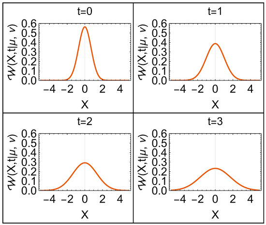
Figure 1.
Tomographic representation of a Gaussian wave packet for the free particle at different times . Here, the parameters were , , , and .
2.2. Finite Potential Well
Another example where we can obtain the tomographic representation is the finite potential well; it is a potential given by the function
with being a positive constant. This problem allows one to obtain odd and even solutions given the symmetry of the potential well. The general solutions are usually obtained for three regions in the position space: , , and ; they read as
For all the eigenfunctions, one has the relations and , while for odd (even) solutions, one has the parameters (). Additionally, the normalization constants A, , and B are defined as
To obtain the tomographic representation of the wave functions, we separate the tomogram integral of Equation (1) in three regions: , , and . For the odd wave functions, one obtains the following integrals:
and an analogous expression is found for the even states. The following integrals can be obtained for the regions outside of the barrier:
while inside the barrier, one has the following expressions for the even states:
and this integral for odd states inside the barrier:
Then, using Equations (1), (23), and (24), one can plot the tomographic representation of the even and odd states of the finite potential well. In Figure 2 and Figure 3, we show the behaviors of the tomograms for the even and odd solutions of the problem. In these figures, one can see the combination of the position and momentum probability distributions. These tomograms have maxima around the well borders, such as in the momentum probability distribution, and local maxima at the origin and other localized points inside the well, such as in the position probability distribution.
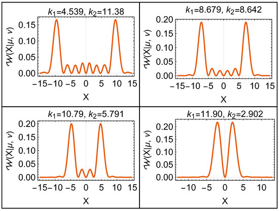
Figure 2.
Tomographic representation of the first four eigenfunctions for the finite potential well (odd solutions) with . Here, the parameters were , , and .

Figure 3.
Tomographic representation of the first four eigenfunctions for the finite potential well (even solutions) with . Here, the parameters were , , and .
2.3. Infinite Potential Well
Another interesting example is the non-symmetrical infinite potential well. In this case, the problem is defined by the potential
which defines the following asymmetrical eigenfunctions of the system:
In view of this expression, we obtain the tomographic representation which, in this case, can be determined using the following integral:
expressed in terms of the imaginary error function. Using Equations (1), (26), and (27), the result is given by the following equation:
In Figure 4, we show the tomographic representation of the first four wave functions for the infinite well. One can see that as in the finite potential well discussed above, there is a combination of the momentum and position probability distributions, where the momentum probability has maxima at the borders of the potential and the position probability has maxima at localized points related to the quantum number n. In contrast with the solutions in the position representation, which should be zero at , the tomographic representation goes asymptotically to zero as the variable X goes to plus or minus infinity. This behavior is also due to the momentum contribution of the tomogram.
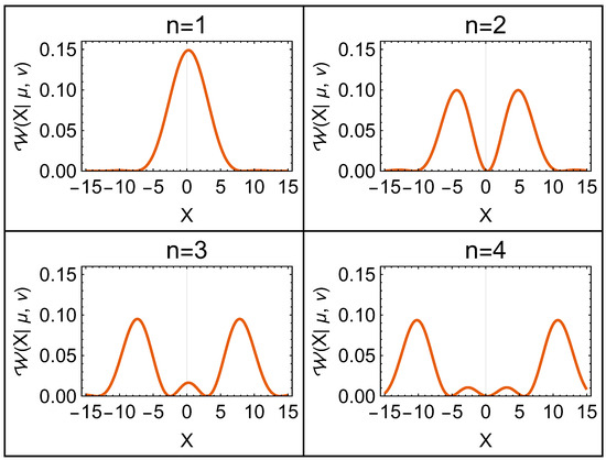
Figure 4.
Tomographic representation of the first four eigenfunctions for the infinite potential well. The parameters used for this representation were , , and .
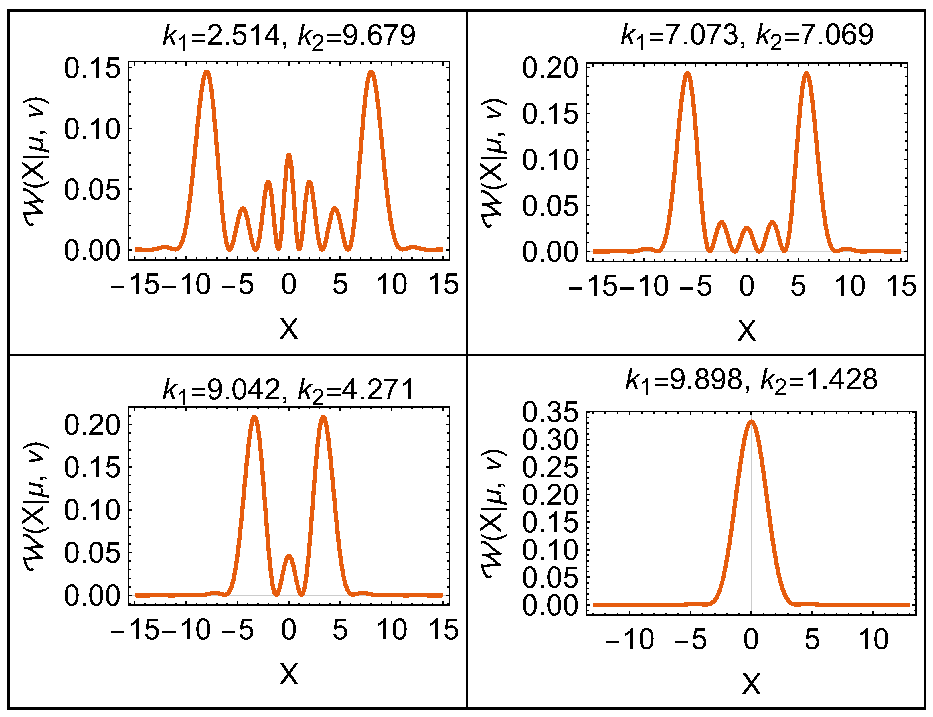
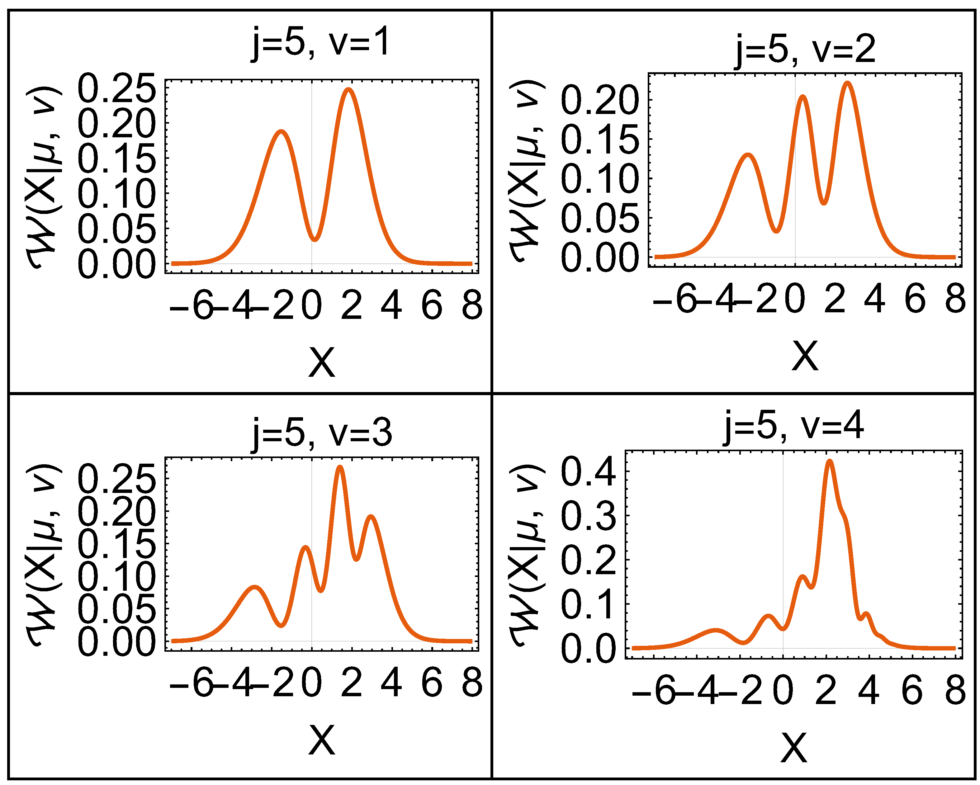
2.4. Morse Potential
Our last example is the phenomenological molecular potential given by the Morse potential. The Morse potential, which reads as [35,36]
where D is the depth of the potential, and is associated with the range of the potential. The bound solutions of this potential are given by
where is a nonnegative integer and j is a positive real number; both numbers are related to the energy, depth, and range of the potential as follows:
with m being the reduced mass of a molecule. The tomographic representation of the solutions of the Morse potential can be numerically found. As an example, we obtained the tomographic representation of the Morse potential solutions with and .
In Figure 5, the numerical solutions for the tomographic representations of four eigenfunctions at are shown. One can observe the complexity of the tomographic representation for the states. This complexity was bigger as the parameter v increased. We point out that the maximum of the tomographic probability distribution is located around the potential minimum, which coincides with the position probability distribution.
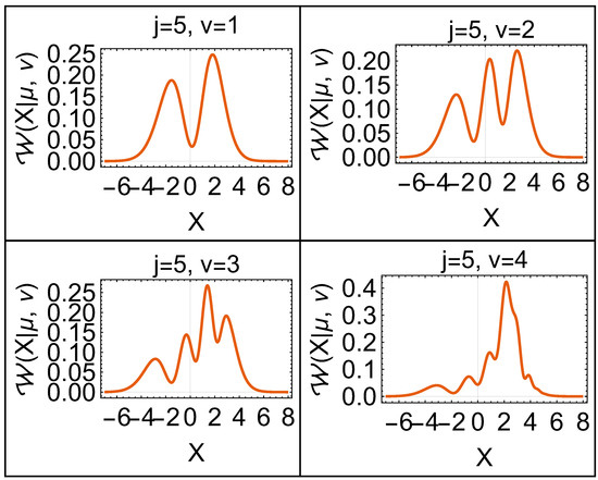
Figure 5.
Tomographic representation for four different states, with solutions of the Morse potential for . In this plot, the parameters used were , , , and .
3. Separability Criteria for Asymmetric Real States
The tomographic representation of quantum mechanics is useful to obtain information about the system using probabilities. At the same time, other probability distributions for a quantum system give different information about its behavior. In this section, we study the momentum probability representation and its relationship to the separability properties of specific bipartite systems.
Let us consider an arbitrary n-partite wave function in the position representation
where the integers , , characterize a particular state; is a normalization constant; and the set of states form an orthogonal basis of functions. It is known that this state, together with its conjugate, must satisfy the probability conservation equation
where we can express the gradient for a system of unidimensional particles as . This probability conservation implies that in the case of stationary states, the divergence of the probability current is equal to zero:
In particular, this stationary probability conservation equation can be satisfied for quantum systems, where the probability current is equal to zero:
For this type of system, one can prove the following theorem for the total momentum probability distribution and reduced momentum probability distributions .
Theorem 1.
For a stationary system with and depicted by an asymmetric wave function , with the momentum representation written as
in a momentum domain , the total momentum probability distribution and the reduced momentum probability distributions are even functions of the momentum variables. That is, and , .
Proof.
To demonstrate the property for a unidimensional system, one first integrates Equation (35) at the position x, that is,
where j can be rewritten with the help of the Dirac notation, and the momentum operator properties and , namely,
which, along with the completeness condition , allows us to write the integral of the probability current:
since the mean value of the momentum operator can be written in an integral form using the momentum probability distribution as follows:
where p is an antisymmetric function; then, must be a symmetric function. This shows the theorem for a unimodal and unidimensional system.
In the n-partite, multidimensional case, one can prove this theorem for each component of , which reduces to the unidimensional case. □
In particular, any asymmetric real wave function satisfies the previous theorem, and therefore, this aspect can be written as the following corollary.
Corollary 1.
Any asymmetric real wave function in the position domain has an even probability distribution in the momentum domain and even reduced momentum probability distributions.
This property can be extended for any real density matrix since, in general, any real can be constructed by a convex sum of products of real wave functions as follows:
where is a real function. Then, the density matrix of Equation (40) in the momentum representation reads
with every superposed momentum probability distribution being an even function of the momentum, as given by Theorem 1. Then, the probability distribution
is a convex sum of even functions, which is also an even function. These arguments can be summarized in the following corollary.
Corollary 2.
Any asymmetric (a state with at least one asymmetrical reduced probability distribution ) real density matrix has an even momentum probability distribution and even reduced momentum probability densities .
Stressing the importance of this corollary for our study, we give a more detailed proof in Appendix A.
Then, the theorem and corollaries above can be used to examine the entanglement of a bipartite system, which can be described by an asymmetric real density matrix. The idea behind this is to explore the symmetries in the momentum space of an asymmetric density matrix under the partial inversion of one of its momentum variables: either or . This property can be given as the following theorem.
Theorem 2.
A necessary condition of separability for a bipartite asymmetric real density matrix is whether the probability distribution of the system is symmetric under both partial momentum inversions and . In other words, .
Proof.
Any real asymmetrical bipartite separable density matrix can be written as a convex sum:
where and are real and define at least one asymmetrical reduced position probability distribution; thus, using the results of Corollary 2, the reduced momentum probability distributions and are even functions. In other words, the transformations
map density matrices into density matrices.
On the other hand, to demonstrate that if a real asymmetrical bipartite density matrix does not obey the Peres–Horodecki criterion [37,38,39] for separability, then the bipartite momentum probability distribution may not be symmetrical on at least one partial momentum inversion (either or ), we can first take into account a general entangled state using the harmonic oscillator basis (without loss of generality):
This leads us to the following bipartite momentum probability distribution:
where the momentum eigenfunctions of the harmonic oscillator are
and they have the same symmetry properties as the position eigenfunctions: . The Hermitian condition of Equation (45) implies , and the normalization condition is represented by . The non-separability of the system can be summarized using the Peres–Horodecki criteria: the partial transpose density matrices and may not represent a well-defined quantum system when the system is non-separable.
Given these properties, the symmetry under the partial inversions and of the bipartite momentum probability can be directly obtained from Equation (46) as follows:
which may be equal to the original probability distribution if both
this may be satisfied if the pairs n and and m and are both even–even and/or odd–odd numbers always (the system has symmetrical position probability distributions) or when, given the correspondence , one has
which means that the partial transpose operations and are bona fide density matrices, and thus, the system is separable (for more details, see Appendix B), contradicting our initial suppositions of asymmetry and non-separability. So, we conclude that holds for a real density matrix only when the system is separable or when it has a defined symmetry for both subsystems ( and ). □
The necessary separability condition given in Theorem 2 is also a sufficient criterion in the cases where the Peres–Horodecki criterion is a sufficient condition for separability. These cases include the following conditions: when the sums of the parameters n and have two contributions and m and have two or three elements.
This separability criterion may allow us to detect bipartite entanglement directly using the momentum probability distribution of the system, and thus, may be more convenient when working with continuous variable systems. On the other hand, this criterion may have implications in the probabilistic representation given by the tomogram. As we have discussed, the tomogram contains information on both the position and momentum probability distributions.
Example
For a better understanding of our results, we present a specific example of our separability criteria. Let us suppose a two-mode harmonic oscillator state of the form
which is not a factorizable state but may be separable. One can obtain the reduced density matrices
where these define a symmetric probability function for mode 1 and an asymmetrical probability function for mode 2 in the position representation. In other words, this density matrix is real and asymmetric, as established by Theorem 2.
The momentum probability distribution of this system is then given by the function
which a symmetric function of both and . From this result and Theorem 2, one can conclude that this system is separable. This can be corroborated, as the system can be expressed as the following convex sum of product states:
with the states . Similarly to this example, more complicated states can be taken into account and their separability information may be obtained by examining the symmetry of the momentum probability distribution.
4. Summaryand Concluding Remarks
In the present paper, we briefly review our collaboration works between the Lebedev Institute and the Mexican research group at UNAM. Different contributions related to the tomographic representation of quantum dynamics, dynamics of superposition of coherent states, and geometric representations of quantum systems are mentioned.
In this contribution, the construction of probability distributions describing quantum system states is considered. The states are formally described either by vectors or by density operators acting in a Hilbert space. It turns out that there exists an invertible map of the vectors and density operators onto probability representations, which are used in our article for concrete systems using wave functions describing the state vectors. This idea can be used for any other quantum system. In particular, we present new results associated with the tomographic representation of wave functions for different potentials, such as the free particle, the finite and infinite potential wells, and the Morse potential. We discuss some of their properties and behavior since the tomographic representation has information on both the position and momentum probability distributions. In most of the cases, we provide the explicit expressions for the tomogram of the system.
Finally, we present a discussion of separability in a bipartite asymmetrical real system, which leads us to provide a new criterion using the symmetry properties of the momentum probability distribution that may be used to distinguish separability in a continuous variable system. In particular, this new criterion tells us that a necessary condition for the separability of a real, bipartite system is that the momentum probability distribution satisfies and can be applied in the cases where at least one of the reduced position probability distributions is not symmetrical ( or ). This criterion corresponds to the Peres–Horodecki criterion applied to the momentum probability distribution and it is a sufficient condition in different systems.
We plan to extend our analysis of the probability representation of quantum systems in the cases where the behavior of wave functions is known. For example, since the quasiclassical approximation of wave functions is well developed, we hope to use the quasiclassical expressions for wave functions and obtain the relation of wave functions to tomograms and find the quasiclassical expression for a symplectic tomogram in all known cases of quasiclassical solutions for quantum systems. This can provide a new approach for considering quasiclassical probability distributions known in probability theory. Also, we will propose how to find corrections to the tomograms corresponding to approximated solutions to the Schrödinger equation connected with approximated solutions to the equations for quantum tomograms. We will present such results in future publications.
Author Contributions
Conceptualization, J.A.L.-S., M.A.M. and V.I.M.; methodology, J.A.L.-S., M.A.M. and V.I.M.; formal analysis, J.A.L.-S., M.A.M. and V.I.M.; investigation, J.A.L.-S., M.A.M. and V.I.M.; writing—original draft preparation, J.A.L.-S., M.A.M. and V.I.M.; writing—review and editing, J.A.L.-S., M.A.M. and V.I.M.; visualization, J.A.L.-S., M.A.M. and V.I.M. All authors have read and agreed to the published version of the manuscript.
Funding
J.A.L.-S. wants to acknowledge the partial support from the Priority 2030 program at the National University of Science and Technology “MISIS” under Project K1-2022-027.
Data Availability Statement
No new data was created.
Acknowledgments
J.A.L.-S. wants to thank Octavio Castaños, Sergio Cordero, Ramón López-Peña, and Eduardo Nahmad-Achar at ICN-UNAM for their extensive discussions and suggestions.
Conflicts of Interest
Author J.A.L.-S. was employed by the company Russian Quantum Center. The remaining authors declare that the research was conducted in the absence of any commercial or financial relationships that could be construed as a potential conflict of interest.
Appendix A
To prove Corollary 2 of Theorem 1 for real, asymmetric density matrices, we can use any complete basis in the position representation. It is convenient to use the harmonic oscillator basis since its symmetry is known and is conformed by real wave functions .
A general real state can be represented by the density matrix
where the parameter matrix is real and symmetrical (, ), and the property follows from the normalization condition.
Since we take into account only asymmetrical states , this means that our matrix cannot be formed by only n and m as both even or both odd; that is,
for any n and m. This property has implications for the momentum representation of the system, which one can write, following Equation (A1), as
One can separate the asymmetrical state (A3) into parts with different symmetries and evaluate the momentum probability distribution as follows:
which can be reduced to only the even–even plus the odd–odd terms since the even–odd and odd–even cancel each other as follows:
Thus, finally we conclude that an arbitrary asymmetrical real density matrix of Equation (A1) has a symmetrical momentum probability distribution expressed by
It is important to notice that when the system is symmetric ( has only even–even and/or odd–odd contributions), then the momentum probability distribution will also be symmetric. However, only the separability properties of bipartite real and asymmetrical states can be evaluated using their momentum probability distribution and, because of this fact, we emphasize the asymmetry of the system.
Appendix B
For the sake of clarity, we explicitly show that the condition of Equation (50) implies the separability of the state of Equation (45). The state of Equation (45) and its partial transpositions can be written in the Dirac form as follows:
After changing the variables and in the expression for and and in the expression for , we arrive at
which can be changed back using the old indices and in the expression for and and in the expression for , resulting in
thus, if Equation (50) holds, then the partial transpositions are equal to the original state , and the system may be separable, as supported by the Peres–Horodecki criterion.
References
- Feder, T. 2025 is the International Year of Quantum Science and Technology. Phys. Today 2025, 78, 7. [Google Scholar] [CrossRef]
- Castaños, O.; López-Peña, R.; Man’ko, V.I. Schrödinger cat states of a non-stationary generalized oscillator. J. Phys. A Math. Gen. 1996, 29, 2091. [Google Scholar] [CrossRef]
- Castaños, O.; López-Peña, R.; Man’ko, V.I. Crystallized Schrödinger cat states. Russ. Laser Res. 1995, 16, 477. [Google Scholar] [CrossRef]
- Castaños, O.; López-Peña, R. Quantum-Like Models and Coherent Effects; Fedele, R., Shukla, P.K., Eds.; World Scientific Publishing: Singapore, 1995; pp. 3–17. [Google Scholar] [CrossRef]
- Castaños, O.; López-Peña, R.; Man’ko, V.I. Variational formulation of linear time-dependent invariants. Europhys. Lett. 1996, 33, 497. [Google Scholar] [CrossRef]
- Castaños, O.; Jáuregui, R.; López-Peña, R.; Recamier, J.; Man’ko, V.I. Schrödinger-cat states in Paul traps. Phys. Rev. A 1997, 55, 1208. [Google Scholar] [CrossRef]
- Castaños, O.; Hacyan, S.; López-Peña, R.; Man’ko, V.I. Schrödinger cat states in a Penning trap. J. Phys. A Math. Gen. 1998, 31, 1227. [Google Scholar] [CrossRef]
- Man’ko, O.V.; Man’ko, V.I. Quantum states in probability representation and tomography. J. Russ. Laser Res. 1997, 18, 407. [Google Scholar] [CrossRef]
- Castaños, O.; Hacyan, S.; López-Peña, R.; Man’ko, M.A.; Man’ko, V.I. Kernel of star-product for spin tomograms. J. Phys. A Math. Gen. 2003, 36, 4677. [Google Scholar] [CrossRef]
- Castaños, O.; López-Peña, R.; Man’ko, M.A.; Man’ko, V.I. Nonstationary linear spin systems in the probability representation. J. Opt. B Quantum Semiclass. Opt. 2003, 5, 227. [Google Scholar] [CrossRef]
- Castaños, O.; López-Peña, R.; Man’ko, M.A.; Man’ko, V.I. Squeeze tomography of quantum states. J. Phys. A Math. Gen. 2004, 37, 8529. [Google Scholar] [CrossRef]
- López-Saldívar, J.A.; Figueroa, A.; Castaños, O.; López-Peña, R.; Man’ko, M.A.; Man’ko, V.I. Discretization of the Density Matrix as a Nonlinear Positive Map and Entanglement. J. Russ. Laser Res. 2016, 37, 313. [Google Scholar] [CrossRef]
- López-Saldívar, J.A.; Figueroa, A.; Castaños, O.; López-Peña, R.; Man’ko, M.A.; Man’ko, V.I. Evolution and Entanglement of Gaussian States in the Parametric Amplifier. J. Russ. Laser Res. 2016, 37, 23. [Google Scholar] [CrossRef]
- Figueroa, A.; López-Saldívar, J.A.; Castaños, O.; López-Peña, R. Extremal Density Matrices for Qudit States. arXiv 2016, arXiv:1609.09835. [Google Scholar]
- Castaños, O.; Figueroa, A.; López, J.; López-Peña, R. Extremal density matrices for the expectation value of a qudit hamiltonian. J. Phys. Conf. Ser. 2017, 839, 012012. [Google Scholar] [CrossRef]
- Figueroa, A.; López-Saldívar, J.; Castaños, O.; López-Peña, R.; Man’ko, M.A.; Man’ko, V.I. Entropy–energy inequalities for qudit states. J. Phys. A Math. Theor. 2015, 48, 065301. [Google Scholar] [CrossRef]
- López-Saldívar, J.; Castaños, O.; Man’ko, M.A.; Man’ko, V.I. Entropic bounds between two thermal equilibrium states. Phys. Rev. E. 2018, 97, 022128. [Google Scholar] [CrossRef] [PubMed]
- López-Saldívar, J.A.; Castaños, O.; Man’ko, M.A.; Man’ko, V.I. New entropic inequalities for qubit and unimodal Gaussian states. Phys. A 2018, 491, 64. [Google Scholar] [CrossRef]
- López-Saldívar, J.; Castaños, O.; Nahmad-Achar, E.; López-Peña, R.; Man’ko, M.A.; Man’ko, V.I. Geometry and entanglement of two-qubit states in the quantum probabilistic representation. Entropy 2018, 20, 630. [Google Scholar] [CrossRef]
- López-Saldívar, J.A.; Castaños, O.; Man’ko, M.A.; Man’ko, V.I. A new mechanism of open system evolution and its entropy using unitary transformations in noncomposite qudit systems. Entropy 2019, 21, 736. [Google Scholar] [CrossRef]
- López-Saldívar, J.A.; Castaños, O.; Man’ko, M.A.; Man’ko, V.I. Qubit representation of qudit states: Correlations and state reconstruction. Quantum Inf. Process. 2019, 18, 210. [Google Scholar] [CrossRef]
- Schrödinger, E. Quantisierung als Eigenwertproblem (Erste Mitteilung). Ann. Phys. 1926, 384, 361–376. [Google Scholar] [CrossRef]
- Schrödinger, E. Quantisierung als Eigenwertproblem (Zweite Mitteilung). Ann. Phys. 1926, 384, 489–527. [Google Scholar] [CrossRef]
- Landau, L. Das Dämpfungsproblem in der Wellenmechanik. Z. Phys. 1927, 45, 430–441. [Google Scholar] [CrossRef]
- Von Neumann, J. Wahrscheinlichkeitstheoretischer Aufbau der Quantenmechanik. Nachrichten von der Gesellschaft der Wissenschaften zu Göttingen, Mathematisch-Physikalische Klasse. 1927. Volume 1927, pp. 245–272. Available online: http://eudml.org/doc/59230 (accessed on 7 January 2025).
- Mancini, S.; Man’ko, V.I.; Tombesi, P. Symplectic tomography as classical approach to quantum systems. Phys. Lett. A 1996, 213, 1–6. [Google Scholar] [CrossRef]
- Man’ko, V.I.; Mendes, R.V. Non-commutative time-frequency tomography. Phys. Lett. A 1999, 263, 53–61. [Google Scholar] [CrossRef]
- Man’ko, M.A.; Man’ko, V.I.; Mendes, R.V. A probabilistic operator symbol framework for quantum information. J. Russ. Laser Res. 2006, 27, 507–532. [Google Scholar] [CrossRef]
- Wigner, E. On the quantum correction for thermodynamic equilibrium. Phys. Rev. 1932, 40, 749–759. [Google Scholar] [CrossRef]
- Husimi, K. Some formal properties of the density matrix. Proc. Phys. Math. Soc. Jpn. 1940, 22, 264–314. [Google Scholar] [CrossRef]
- Dodonov, V.V.; Man’ko, V.I. Positive distribution description for spin states. Phys. Lett. A 1997, 229, 335–339. [Google Scholar] [CrossRef]
- Landau, L.D. The damping problem in wave mechanics. In Collected Papers of L.D. Landau; Pergamon: Berlin, Germany, 1965; pp. 8–18. [Google Scholar] [CrossRef]
- Sakurai, J.J.; Napolitano, J. Modern Quantum Mechanics; Cambridge University Press: Cambridge, UK, 2021; p. 118. [Google Scholar] [CrossRef]
- Zee, A. Quantum Field Theory in a Nutshell; Princeton University Press: Princeton, NJ, USA, 2010; p. 523. [Google Scholar]
- Morse, P.M. Diatomic molecules according to the wave mechanics. II. Vibrational levels. Phys. Rev. 1929, 34, 357. [Google Scholar] [CrossRef]
- Lemus, R.; Arias, J.M.; Gómez-Camacho, J. An su(1, 1) dynamical algebra for the Morse potential. J. Phys. A Math. Gen. 2004, 37, 1805. [Google Scholar] [CrossRef]
- Peres, A. Separability criterion for density matrices. Phys. Rev. Lett. 1996, 77, 1413. [Google Scholar] [CrossRef] [PubMed]
- Horodecki, M.; Horodecki, P.; Horodecki, R. Separability of mixed states: Necessary and sufficient conditions. Phys. Lett. A 1996, 223, 1. [Google Scholar] [CrossRef]
- Horodecki, R.; Horodecki, P.; Horodecki, M.; Horodecki, K. Quantum entanglement. Rev. Mod. Phys. 2009, 81, 865. [Google Scholar] [CrossRef]


Disclaimer/Publisher’s Note: The statements, opinions and data contained in all publications are solely those of the individual author(s) and contributor(s) and not of MDPI and/or the editor(s). MDPI and/or the editor(s) disclaim responsibility for any injury to people or property resulting from any ideas, methods, instructions or products referred to in the content. |
© 2025 by the authors. Licensee MDPI, Basel, Switzerland. This article is an open access article distributed under the terms and conditions of the Creative Commons Attribution (CC BY) license (https://creativecommons.org/licenses/by/4.0/).