Global Chlorophyll Concentration Distribution and Effects on Bottom Reflectance of Coral Reefs

Abstract

Despite the limited coverage of coral reefs in the world’s oceans, they play a crucial role in global marine biodiversity and providing essential ecosystem services. This study explores the influence of chlorophyll-a (Chl-a) concentration in the water column on the estimation of bottom reflectance (r_b) in coral reefs monitored by the Allen Coral Atlas coral reef monitoring system, using satellite imagery from a Sentinel-2 MSI sensor. We conducted a comprehensive analysis, considering Chl-a global distribution and variability, and its combined effect with water column depth over r_b calculation. Our results demonstrated that the impact of Chl-a on r_b estimation becomes significant when the water column depth exceeds 3 m. While suggesting the optionality of using regional Chl-a values, our study highlights potential overestimations of Chl-a in optically complex environments, such as along the Brazilian coast. This research contributes to refining coral reef monitoring systems and underscores the importance of accurate Chl-a assessments for robust environmental evaluations.

1. Introduction

Shallow coral reefs cover a small portion of global oceans but support upwards of 25% of global marine biodiversity [1,2,3,4]. Reefs also support coastal protection, food, and recreation for neighboring human populations as well as being a global-scale food and recreational source [5,6,7]. Despite their significance, coral reef ecosystems face increasing threats such as extensive exploitation, resulting in their global deterioration [8].

Mapping and monitoring coral reefs plays a major role in developing and implementing effective management strategies [9]. Reef bottom reflectance (r_b) provides information needed to monitor changes in benthic composition and state [10]. Multispectral remote sensing continues to be a growing tool for assessing changes in bottom reflectance, but to account for the interference of water in pursuit of the seafloor signal, it is necessary to separate the components of the bottom reflectance from water column scattering and absorption processes.

The Allen Coral Atlas coral reef monitoring system utilizes Sentinel-2 L2A/B satellite imagery to detect changes in benthic color reflectance and to assign detected changes in benthic reflectance to potential coral bleaching. Estimating benthic reflectance requires an effort to minimize the water column signal by estimating the optical properties of the water column. Several algorithms have been implemented to obtain these water column properties, such as absorption and backscattering coefficients, which are highly dependent on the concentration of chlorophyll-a (Chl-a) in seawater (Figure 1). Despite a known dependence of the Allen Coral Atlas coral reef monitoring system on water column Chl-a, the beta version of the Atlas system employed a fixed global Chl-a value of 0.5 mg·m⁻³.

Figure 1. Methodology flowchart used by the Allen Coral Atlas’ to calculate the r_b from Sentinel-2 satellite data. For symbol definitions see

Table 1. Definition of terms, units, and abbreviations.

	Units	Definition
acdom(λ)	m−1	Absorption coefficient of chromophoric dissolved organic mater
anap(λ)	m−1	Absorption coefficient of non-algal particles
aph(λ)	m−1	Absorption coefficient of phytoplankton pigments
at(λ)	m−1	Absorption coefficient of the total (aw + acdom + aph + anap)
aw(λ)	m−1	Absorption coefficient of pure seawater
bbp(λ)	m−1	Backscattering coefficient of suspended particles
bbt(λ)	m−1	Backscattering coefficient of the total, bbw + bbp
bbw(λ)	m−1	Backscattering coefficient of pure seawater
Chl-a	mg·m−3	Chlorophyll-a concentration
Db		Distribution function that relates the vertically averaged diffuse attenuation coefficient for upwelling radiance from bottom reflectance to at and bt
Dc		Distribution function that relates the vertically averaged diffuse attenuation coefficient for upwelling radiance from water-column scattering to at and bt
rrs	sr−1	Below-surface remote sensing reflectance
rrsb	sr−1	Below-surface remote sensing reflectance from bottom reflection
rrsc	sr−1	Below-surface remote sensing reflectance from water column scattering
rrsdeep		Below-surface remote sensing reflectance when the water depth is infinite
rb		Bottom reflectance
Rrs	sr−1	Above-surface remote sensing reflectance

.

Figure 1. Methodology flowchart used by the Allen Coral Atlas’ to calculate the r_b from Sentinel-2 satellite data. For symbol definitions see Table 1.

Here, we aimed to determine the effects of Chl-a on r_b estimation. To achieve this, we addressed two key questions: (1) What is the global distribution and variability of water column Chl-a over coral reefs? (2) How does the variability of Chl-a affect the estimation of r_b on coral reefs? In answering these questions, we sought to improve the Allen Coral Atlas coral reef detection system while also providing general insight on Chl-a estimation that might assist in other oceanographic programs. Our findings contribute to improving our understanding of the current state and the changes underway in coral reef ecosystems worldwide.

2. Materials and Methods

In this study, we target coral reefs gathered within the 214 globally distributed regions of the NOAA-CRW Regional Virtual Stations (https://coralreefwatch.noaa.gov/product/vs/data.php (accessed on 24 March 2023)). These regions encompass numerous geographic locations, capturing the diversity and associated challenges present in coral reef environments worldwide.

Our analysis specifically centers on coral reefs classified as the benthic “coral/algae” category in the Allen Coral Atlas. It is important to note that this category only includes coral reefs to a maximum depth of 10 m, as this is the maximum depth that can be accurately monitored with multispectral satellite imagery [11].

2.1. Satellite Data

We utilized a time series of Sentinel-2 L2A/B satellite data spanning from 1 January 2019 to 31 December 2022. Sentinel-2 MSI provides data with a spatial resolution of 10 m, 20 m, and 60 m. The data were acquired and processed through Google Earth Engine (GEE). GEE retrieves the data from Sentinel Hub and performs the atmospheric correction implementing sen2cor (https://step.esa.int/main/snap-supported-plugins/sen2cor/ (accessed on 24 March 2023)), which also generates a Scene Classification Map (SCL) band with a 20 m resolution. Utilizing information from the SCL and the QA60 (Quality Assessment 60-m resolution) bands provided with the Sentinel-2 imagery, we identified clouds and cloud shadows and masked them out. The QA60 band offers indicators related to cloud probability and atmospheric conditions (https://sentinel.esa.int/web/sentinel/technical-guides/sentinel-2-msi/level-1c/cloud-masks (accessed 24 March 2023)). Additionally, the SCL band categorizes pixels into various land cover classes, including water bodies and clouds, thereby aiding in cloud detection (https://custom-scripts.sentinel-hub.com/custom-scripts/sentinel-2/scene-classification/ (accessed on 24 March 2023)). Leveraging this information, we implemented the maskS2clouds() function from Google Earth Engine (GEE) (https://developers.google.com/earth-engine/datasets/catalog/COPERNICUS_S2_SR (accessed on 24 March 2023)) to generate clean, cloud-free imagery. The maskS2clouds() function internally resamples the cloud and shadow masks derived from the QA60 and SCL bands to match the resolution of the target bands, ensuring accurate application of the masks to all bands.

2.2. Chl-a Calculation

Chl-a is a central component in the computation of r_b. The areas monitored by the atlas are located in the tropical oceans. Generally, tropical reefs occur in highly oligotrophic oceanic water, systems where the water column nutrients are characteristically low [12]. Therefore, to compute the satellite-derived Chl-a from the above-surface remote sensing reflectance (R_rs) we tested the implementation of the approach described by [13]:

$$\mathrm{Chl}\text{-}a={10}^{(-0.4909+191.659\times \omega )}$$

(1)

where $\omega$ is the weighted relative difference between R_rs(443) and R_rs(555), computed as follows:

$$\omega =R_{\mathrm{r}\mathrm{s}}\left(560\right)-0.46\times R_{\mathrm{r}\mathrm{s}}\left(443\right)-0.54\times R_{\mathrm{r}\mathrm{s}}\left(670\right)$$

(2)

In [13], the authors demonstrated the strong correlation between satellite-derived Chl-a and in situ Chl-a over a wide range of concentrations (0.03–10 mg·m⁻³) when applied to MODIS-Aqua satellite data. It has been demonstrated that MODIS-Aqua reflectance is in good agreement with Sentinel-2 L2A/2B MSI reflectance [14]. Thus, we believe this algorithm (Equations (1) and (2)) can be implemented to estimate Chl-a for the Allen Coral Atlas coral reef monitoring system, based on Sentinel-2 L2A/2B MSI data.

The computation of Chl-a was exclusively conducted for pixels within the regional polygons that contain coral reefs. Initially, an image collection was assembled for each region, consolidating data from 1 January 2019 to 31 December 2022, masking clouds and shadows (see Section 2.1). Subsequently, a mask assembling the areas corresponding to the coral/algae class from the benthic maps available on the ACA website (https://allencoralatlas.org/atlas/#1.00/0.0000/-145.0000 (accessed on 24 March 2023)) was generated for each region. Only pixels falling within the coral/algae category were used for subsequent computation.

Bands 2 (490 nm), 3 (560 nm), and 4 (665 nm) were selected and independently averaged, followed by the calculation of Chl-a for each of the remaining pixels. To mitigate the influence of outliers, pixels exhibiting Chl-a values surpassing 100 mg·m⁻³ were systematically excluded, as they deviate from the anticipated Chl-a in the ocean [15]. Moreover, the global mean and standard deviation of Chl-a were computed, establishing a threshold as the global mean plus one standard deviation. Pixels exceeding this threshold were masked.

Finally, for each region, the mean Chl-a (mChl-a) was computed by spatially averaging the pixel values.

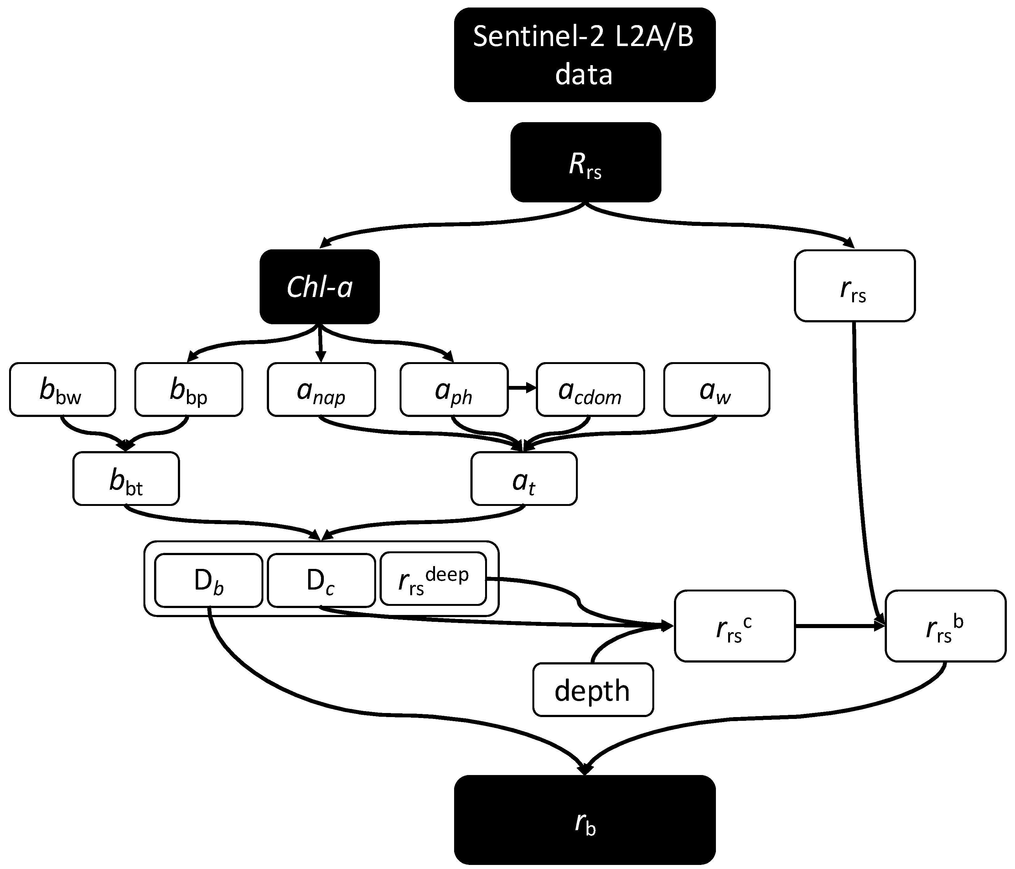
2.3. Bottom Reflectance Calculation

r_b was calculated from above-surface remote sensing reflectance (R_rs) following the methodology proposed by [16]. Their model requires assessing the below-surface remote sensing reflectance (r_rs) and isolating the signal of its contributors: the water column scattering (r_rs^c) and the bottom reflectance (r_rs^b). r_rs were derived from R_rs(λ) as defined by [17].

$$r_{\mathrm{r}\mathrm{s}}(\lambda )=\frac{R_{\mathrm{r}\mathrm{s}}\left(\lambda \right)}{0.52+1.7R_{\mathrm{r}\mathrm{s}}\left(\lambda \right)}$$

(3)

Furthermore, r_rs can also be expressed as the summation of the water column constituent and the bottom constituent (Equation (4)).

$$r_{\mathrm{r}\mathrm{s}}\left(\lambda \right)={r_{\mathrm{r}\mathrm{s}}}^{\mathrm{b}}\left(\lambda \right)+{r_{\mathrm{r}\mathrm{s}}}^{\mathrm{c}}\left(\lambda \right)$$

(4)

$${r_{\mathrm{r}\mathrm{s}}}^{\mathrm{c}}\left(\lambda \right)=r_{\mathrm{r}\mathrm{s}}^{\mathrm{d}\mathrm{e}\mathrm{e}\mathrm{p}}\left(1-e^{-D_{\mathrm{c}}\left(a_{\mathrm{t}}+b_{\mathrm{b}}\right)\mathrm{H}}\right)$$

(5)

$${r_{\mathrm{r}\mathrm{s}}}^{\mathrm{b}}\left(\lambda \right)=\frac{1}{\pi }{r_{\mathrm{b}}\left(\lambda \right)e}^{-D_{\mathrm{b}}(a_{\mathrm{t}}+b_{\mathrm{b}})\mathrm{H}}$$

(6)

In Equations (5) and (6), a_t indicates the total absorption of the water column, b_b represents the total backscattering of the water column, and H denotes the depth of the water column under consideration. For our calculations, we used the satellite-derived depth from the Allen Coral Atlas calculated implementing the methodology described by [18].

Furthermore, D_c stands as an empirical parameter accounting for the under-water photon path elongation due to scattering effects within the water columns ([19]; Equation (7)) and D_b is the light attenuation of the bottom reflectance ([19]; Equation (8)). Lastly, $r_{\mathrm{r}\mathrm{s}}^{\mathrm{d}\mathrm{e}\mathrm{e}\mathrm{p}}$ represents r_rs in infinitely deep water, and it was derived from the total absorption (a_t) and total backscattering (b_b) of the water column (Equation (9)).

$$D_{\mathrm{c}}=1.03{(1+2.4\frac{b_{\mathrm{b}}}{a_{\mathrm{t}}+b_{\mathrm{b}}})}^{0.5}$$

(7)

$$D_{\mathrm{b}}=1.05{(1+5.5\frac{b_{\mathrm{b}}}{a_{\mathrm{t}}+b_{\mathrm{b}}})}^{0.5}$$

(8)

$$r_{\mathrm{r}\mathrm{s}}^{\mathrm{d}\mathrm{e}\mathrm{e}\mathrm{p}}=\left(0.089+0.125\frac{b_{\mathrm{b}}}{a_{\mathrm{t}}+b_{\mathrm{b}}}\right)\frac{b_{\mathrm{b}}}{a_{\mathrm{t}}+b_{\mathrm{b}}}$$

(9)

Hence, by rearranging Equation (6), r_b was formulated as follows:

$$r_{\mathrm{b}}\left(\lambda \right)=\frac{{r_{\mathrm{r}\mathrm{s}}}^{\mathrm{b}}\left(\lambda \right)\ast \pi }{e^{-D_{\mathrm{b}}(a_{\mathrm{t}}+b_{\mathrm{b}})H}}$$

(10)

a_t entails the summation of the absorption from three distinct constituents: the absorption coefficient of pure water (a_w), the absorption of phytoplankton (a_ph(λ)), and the absorption of colored dissolved organic matter (a_cdom(λ)) (Equation (11)).

$$a_{\mathrm{t}}\left(\lambda \right)=a_{\mathrm{w}}\left(\lambda \right)+{\mathrm{a}}_{\mathrm{p}\mathrm{h}}\left(\lambda \right)+a_{\mathrm{n}\mathrm{a}\mathrm{p}}\left(\lambda \right)+a_{\mathrm{c}\mathrm{d}\mathrm{o}\mathrm{m}}\left(\lambda \right)$$

(11)

While a_w is a known value [20], a_ph(λ), a_nap(λ), and a_cdom(λ) are derived from satellite data. As described by [21], a_ph(λ) is determined based on satellite-derived Chl-a

$$a_{\mathrm{p}\mathrm{h}}\left(\lambda \right)=\left[a_0\left(\lambda \right)+a_1\left(\lambda \right)\times ln\left(a_{\mathrm{p}\mathrm{h}}\left(440\right)\right)\right]\times a_{\mathrm{p}\mathrm{h}}\left(440\right)$$

(12)

$$a_{\mathrm{p}\mathrm{h}}\left(440\right)=0.06\times {[Chl-a]}^{0.65}$$

(13)

where a₀(λ) and a₁(λ) are known values from [22] QAA(v5).

Afterwards, a_nap(λ) was derived from a_ph(440) implementing the model formulated by [23,24].

$$a_{\mathrm{n}\mathrm{a}\mathrm{p}}\left(\lambda \right)=a_{\mathrm{n}\mathrm{a}\mathrm{p}}\left(440\right)\times e^{-S_{\mathrm{n}\mathrm{a}\mathrm{p}}(\lambda -440)}$$

(14)

$$a_{\mathrm{n}\mathrm{a}\mathrm{p}}\left(440\right)=0.0124\times {[Chl-a]}^{0.724}$$

(15)

where $e^{-S(\lambda -440)}$ with S_nap = 0.011 is the globally average slope of the exponential function representing the spectral dependence of a_nap.

Similarly, a_cdom(λ) was derived from a_ph(440) implementing the model formulated by [23,24].

$$a_{\mathrm{c}\mathrm{d}\mathrm{o}\mathrm{m}}\left(\lambda \right)=a_{\mathrm{c}\mathrm{d}\mathrm{o}\mathrm{m}}\left(440\right)\times e^{-S(\lambda -440)}$$

(16)

$$a_{\mathrm{c}\mathrm{d}\mathrm{o}\mathrm{m}}\left(440\right)=0.5\times a_{\mathrm{p}\mathrm{h}}\left(440\right)$$

(17)

where $e^{-S(\lambda -440)}$ with S = 0.015 is the globally average slope of locally produced chromophoric dissolved organic matter.

Furthermore, b_bt was calculated as the summation of the backscattering of pure water (b_bw) and the backscattering of particles (b_bp).

$$b_{\mathrm{b}\mathrm{t}}\left(\lambda \right)=b_{\mathrm{b}\mathrm{w}}\left(\lambda \right)+b_{\mathrm{b}\mathrm{p}}\left(\lambda \right)$$

(18)

where b_bw is a known value [25] and b_bp was estimated from satellite-derived Chl-a as described by [24].

$$b_{\mathrm{b}\mathrm{p}}\left(\lambda \right)=\left\{0.002+0.02\left[0.5-0.25\times {log}_{10}\left(Chl\text{-}a\right)\right]\times \left(\frac{550}{\lambda }\right)\right\}\times b_{\mathrm{b}\mathrm{p}}\left(555\right)$$

(19)

$$b_{\mathrm{b}\mathrm{p}}\left(555\right)=0.6\times {\left(Chl\text{-}a\right)}^{0.62}$$

(20)

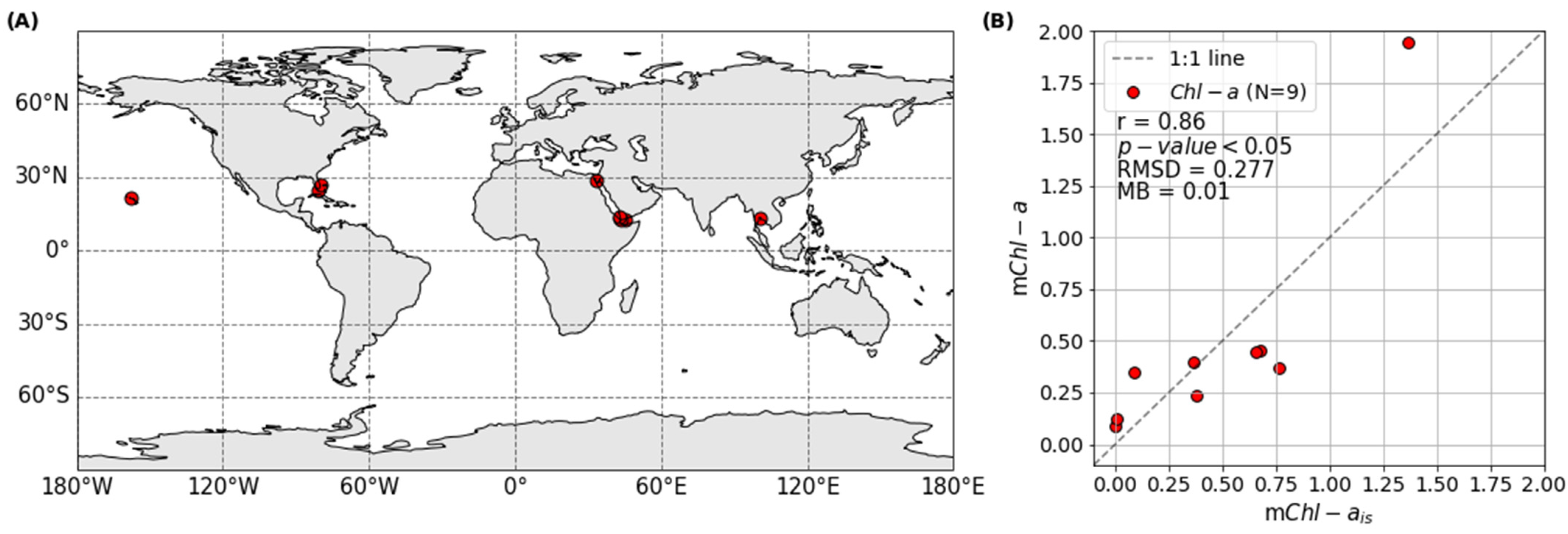
2.4. Satellite-Derived mChl-a Validation

mChl-a validation was conducted by comparing satellite-derived values with an in situ regional mean Chlorophyll-a concentration (mChl-a_is) dataset. The mChl-a_is dataset was built by gathering Chl-a data from the NASA SeaBASS [26] database spanning from the years 2000 to 2022. Notably, the in situ dataset covered a wider time range than that utilized for calculating mChl-a, as there were no matching data available between 2019 and 2022. Additionally, only Chl-a measurements taken up to a depth of 10 m were considered in the analysis, aligning with the maximum depth covered by the Allen Coral Atlas coral bleaching monitoring system. After thoroughly filtering the dataset and averaging the regional in situ Chl-a concentration data, nine matching regions were identified. (Figure 2). Subsequently mChl-a_is was compared to the satellite-derived mChl-a values to assess the accuracy of our estimation (see Section 3).

This evaluation involved visually comparing mChl-a versus mChl-a_is, supported by the Pearson correlation coefficient (r), the root mean square deviation (RMSD, Equation (21)), and the mean bias (MB, Equation (22)).

$$\mathrm{RMSD}=\sqrt{{\sum }_{i=1}^N\frac{{\left(yi-xi\right)}^2}{n}}$$

(21)

$$\mathrm{MB}=\sqrt{\frac{mean\left(yi\right)}{mean\left(xi\right)}}$$

(22)

where yi and xi are the estimated and in situ values, respectively.

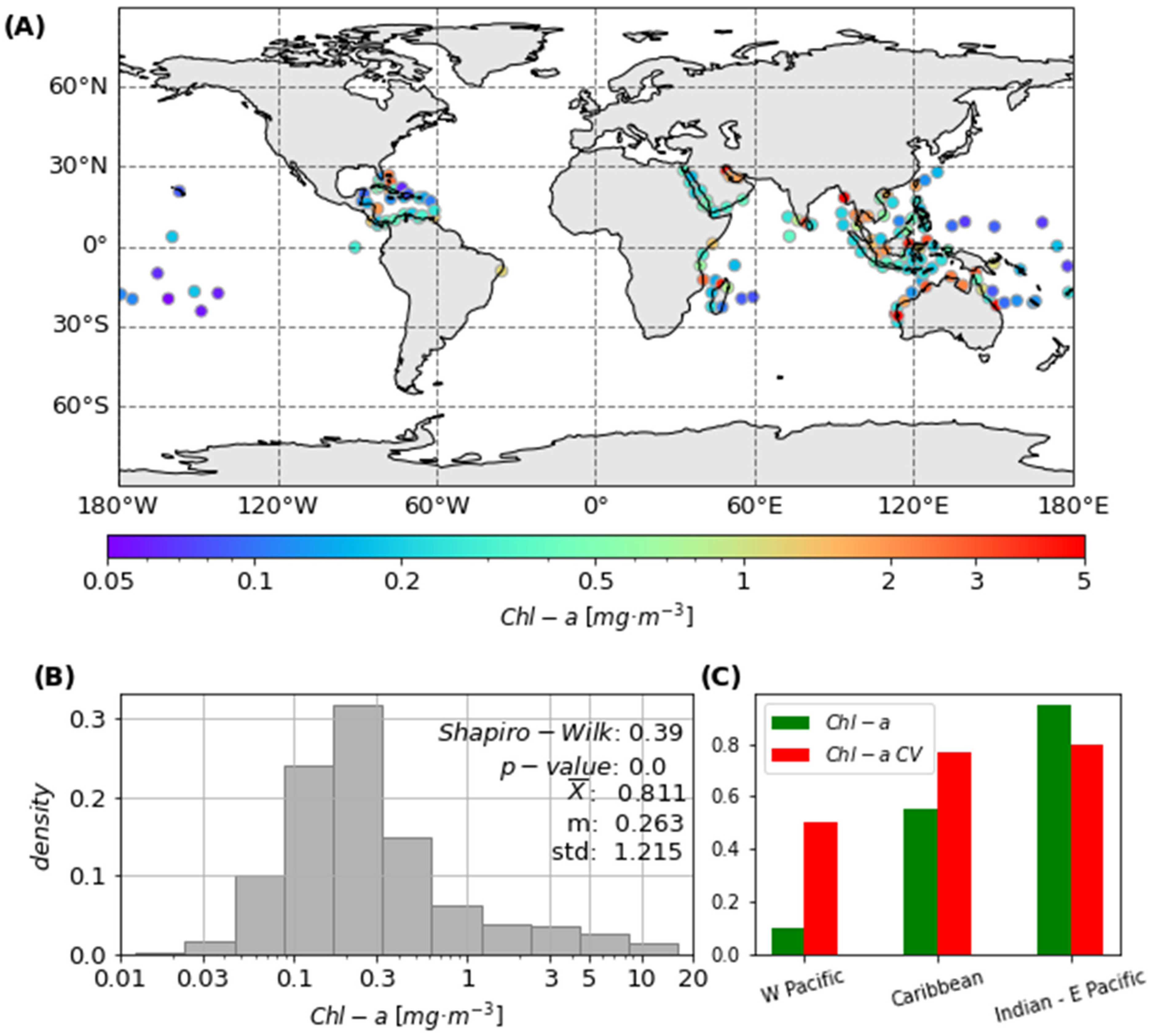
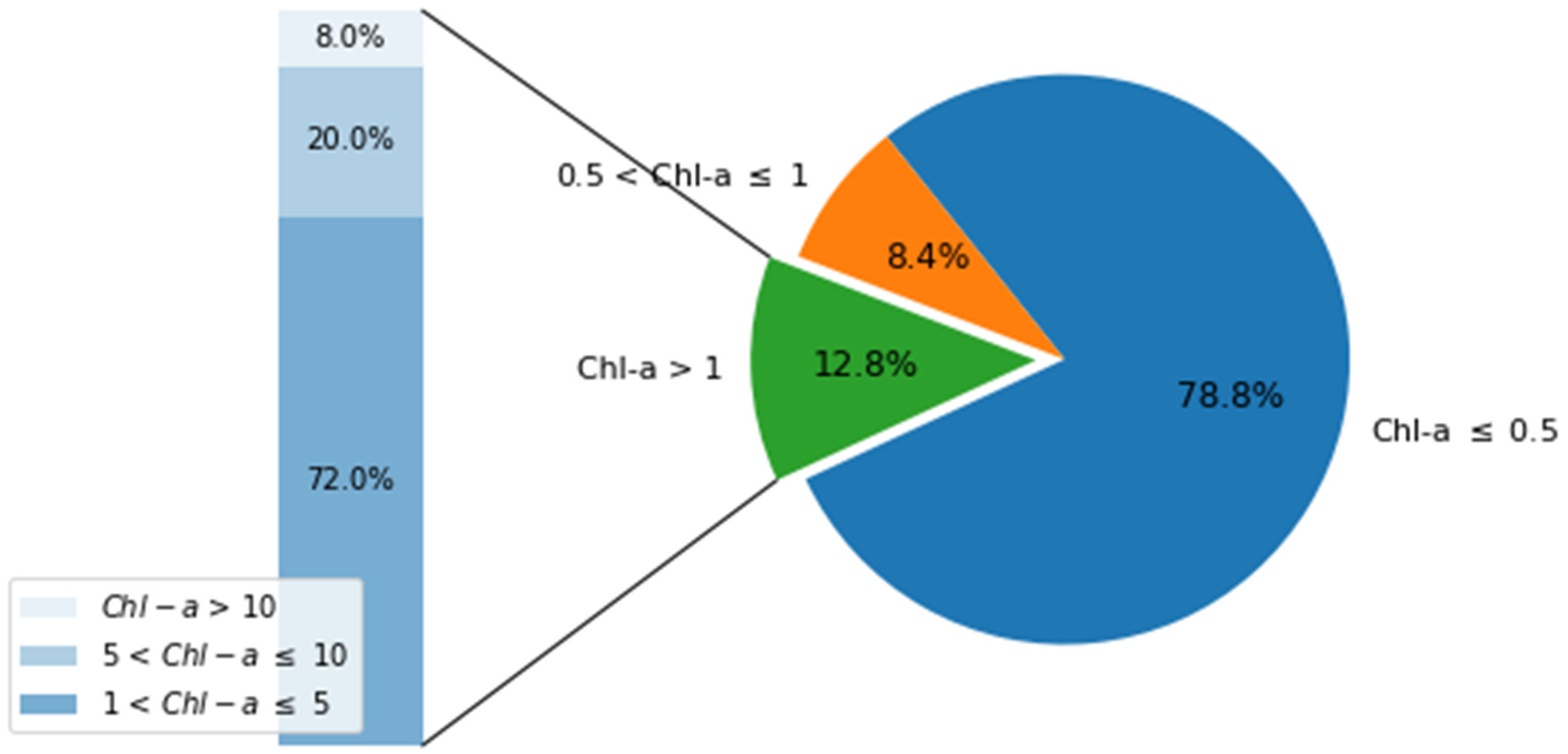
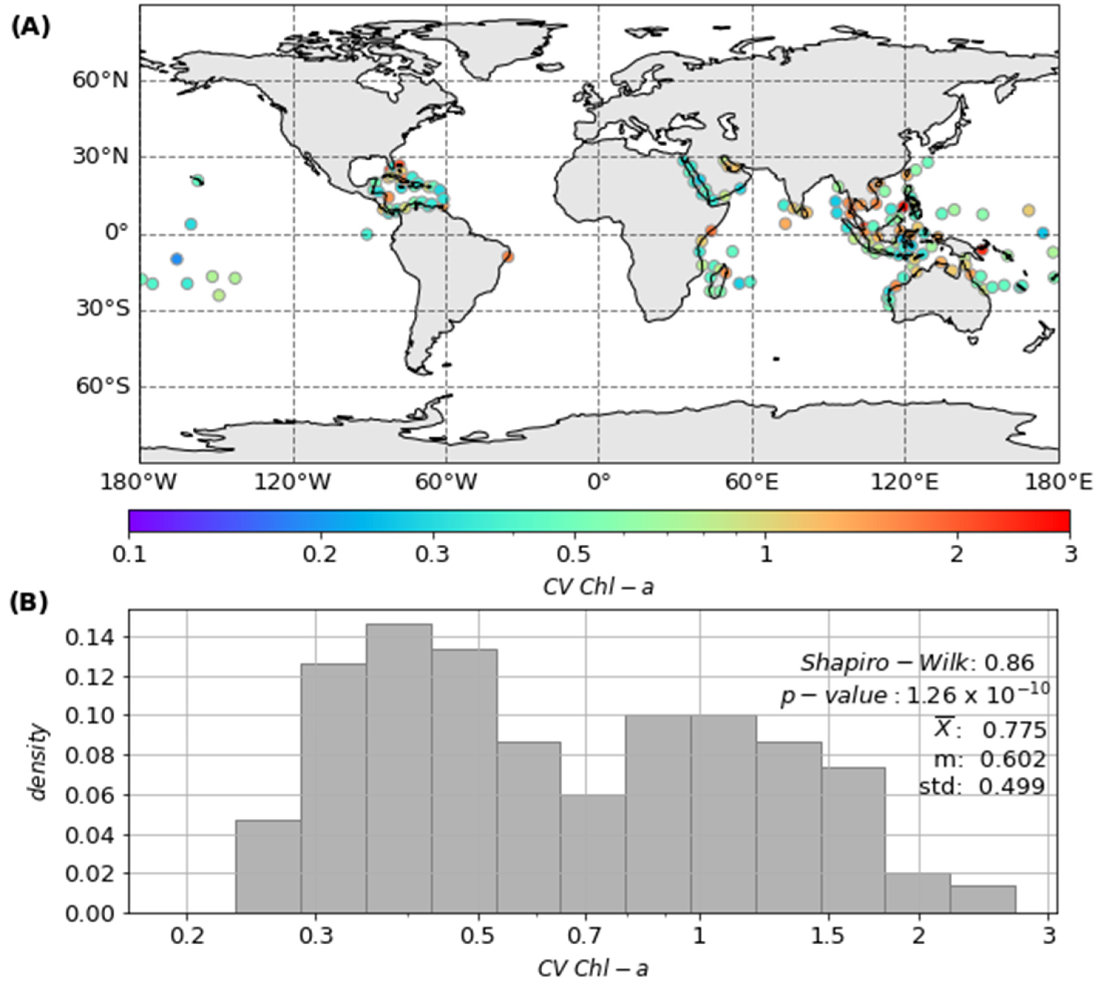
2.5. Satellite-Derived Chl-a Spatial Distribution Variability

A global map of satellite-derived mChl-a was generated, and its distribution and variability were assessed through a combination of graphical analysis and quantitative statistical metrics. First, mChl-a distribution was visualized via a histogram plotted alongside a map displaying mChl-a values. The normality of the distribution was tested using the Shapiro–Wilk test [27], and descriptive statistics including the global mean ($\overline{X}$), median (m), and standard deviation (std) were calculated.

Furthermore, mChl-a was categorized into three classes: values lower than 0.5 mg·m⁻³, between 1 and 0.5 mg·m⁻³, and higher than 1 mg·m⁻³, considering as first boundary the value of Chl-a used in the beta version (0.5 mg·m⁻³); and as second boundary the third quantile of the dataset. A pie chart was utilized to represent the percentage of mChl-a falling into each category.

Additionally, the regional coefficient of variation of Chl-a (Chl-a CV, Equation (23)) was computed at each region to assess both homogeneity and temporal variability.

$$\mathit{Chl}\text{-}aCV=\frac{\sigma }{\mu }$$

(23)

where σ represents the standard deviation of the dataset and μ denotes the mean.

Similarly, the regional CV of Chl-a was mapped, and a histogram was generated to depict its distribution. Additionally, Chl-a CV values were grouped into oceanic basins to investigate global variability patterns.

2.6. Sensitivity Analysis

To evaluate the influence of Chl-a, depth, and R_rs(560) variability on r_b estimation, we generated five synthetic datasets using a revised Saltelli sampling sequence approach [28,29,30,31] (

Table 2. Description of the datasets produced for the sensitivity analysis and for the evaluation of the comparison satellite-derived Chl-a concentration implementing a regional mChl-a vs. using Chl-a fixed at 0.5 mg·m⁻³.

Dataset	Chl-a [mg·m−3]	Rrs(560) [sr−1]	Depth [m]
rb-syn new	range = [0–20]	0.0105 (fixed)	range = [0–10]
rb-syn new (0–1)	range = [0–1]	range = [0.009–0.012]	range = [0–10]
rb-syn new (0–10)	range = [0–10]	range = [0.009–0.012]	range = [0–10]
rb-syn new (0–20)	range = [0–20]	range = [0.009–0.012]	range = [0–10]
rb-syn beta	0.5 (fixed)	range = [0.009–0.012]	range = [0–10]

). This method produces quasi-random sequences of size $n\times (2p+2)$, where p represents the number of input parameters, and n is the baseline sample size. For this study, we selected a sample size of 100, which is considered adequate for reliable index estimation. The synthetic datasets were generated based on the distribution limits of satellite-derived Chl-a and R_rs(560) observed in the evaluated regions between 1 January 2019 and 31 December 2022. The depth range was delimited from 0 to 10 m to align with the coverage of the Allen Coral Atlas coral reef monitoring system.

To examine the combined impact of Chl-a and depth on r_b calculation variability, we generated a synthetic dataset encompassing the entire range of Chl-a (0–20 mg·m⁻³) and depth (0–10 m), and R_rs(560) was fixed at its median (0.0105 sr⁻¹). The synthetic data were used to calculate r_b-syn new.

Additionally, to further broaden the assessment of r_b calculation sensitivity to Chl-a variability, while also considering variable R_rs(560) and depth, we generated three additional sets of r_b-syn calculated from synthetic datasets with varying Chl-a concentrations: 0 to 1 mg·m⁻³ (r_b-syn new (0–1)), 0 to 10 mg·m⁻³ (r_b-syn new (0–10)), and 0 to 20 mg·m⁻³ (r_b-syn new (0–20)). In each case, we maintained the same sets of R_rs(560) and depth, ranging from 0.009 to 0.012 sr⁻¹ and m 0 to 10 m, respectively. These datasets of R_rs(560) and depth were also utilized to calculate r_b-syn beta (with fixed Chl-a of 0.5 mg·m⁻³), and compare it to r_b-syn new (0–1), r_b-syn new (0–10), and r_b-syn new (0–20).

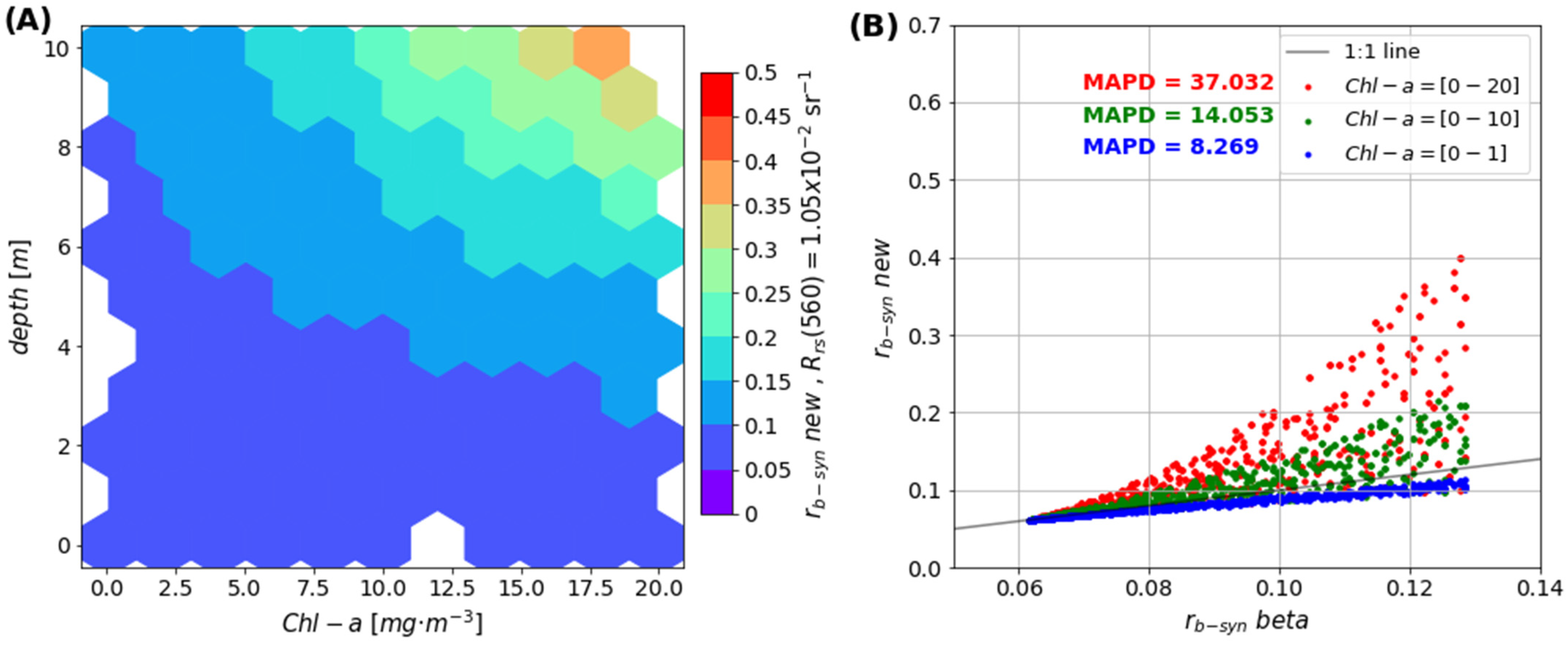
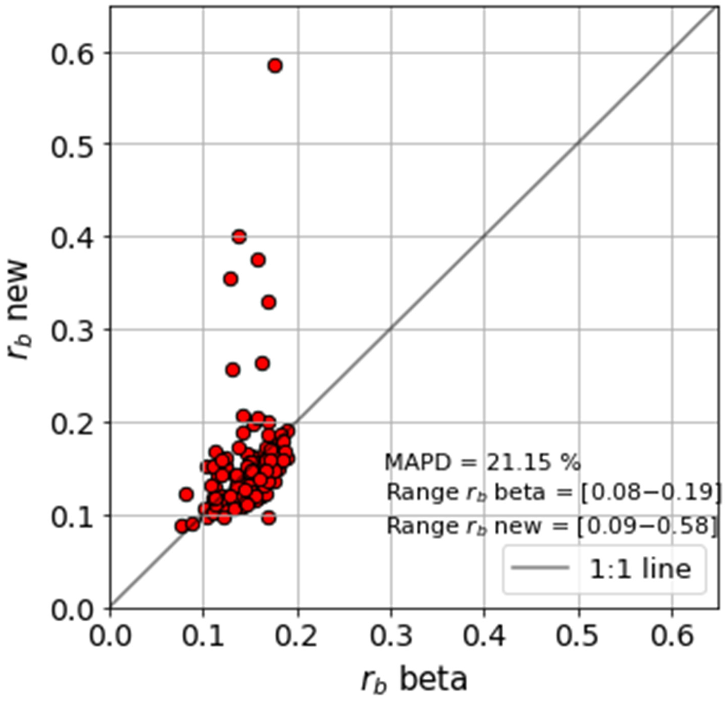
2.7. Comparison of r_b-sat new vs. r_b-sat beta

To better understand the impact of utilizing mChl-a for r_b estimation based on Sentinel-2 L2A/B satellite data, we calculated the mean depth and median R_rs(560) for each monitored region between 1 January 2019 and 31 December 2022. Along with the mChl-a calculated to generate the global map and distribution, we estimated the satellite-derived regional mean r_b (r_b-sat new). r_b-sat new was compared to r_b-sat beta, representing r_b calculated using the same depth and R_rs (560) values, but with Chl-a fixed at 0.5 mg·m⁻³.

We assessed the disparity between r_b new and r_b beta calculating the mean absolute percentage difference (MAPD) (Equation (24)).

$$MAPD=mean{\sum }_{i=1}^N\frac{\left|yi-xi\right|}{xi}\times 100$$

(24)

Here, yi corresponds to r_b-sat new and xi to r_b-sat beta. MAPD provides insights into the extent of the differences between the two sets of estimations.

3. Results

The validation of mChl-a shows that the satellite-derived Chl-a estimation (Figure 2) is reasonable. Nine regions, covering a wide longitudinal range, were effectively matched with in situ Chl-a data collected from 2000 to 2022 (Figure 2). These in situ observations were then regionally averaged to obtain mChl-a_is values (

Table 3. List of Chl-a concentration in situ measurements (mChl-a_is) matched with satellite-derived Chl-a (mChl-a), showing the number of in situ measurements (N) for each region, the year of in situ sampling, and the standard deviation (std) for both satellite (mChl-a std) and in situ (mChl-a_is std) mean regional Chl-a concentration.

Region	N	Year	Mean Depth [m]	mChl-ais [mg·m−3]	mChl-ais std [mg·m−3]	mChl-a [mg·m−3]	mChl-a std [mg·m−3]
Aden	7	2001	0	0.382	0.017	0.234	0.081
East Gulf of Thailand	15	2003	0	1.369	1.973	1.945	2.761
Eritrea	4	2001	0	0.678	0.087	0.453	0.152
Florida Keys	293	2011, 2016–2021	1.49	0.087	0.169	0.345	0.758
Gulf of Suez	85	2001	0	0.367	0.327	0.395	0.134
Gulf of Tadjoura	10	2001	0	0.762	0.044	0.372	0.107
Hawaii	1	2017	0	0.002	-	0.086	0.039
Southeast Florida	10	2007, 2012, 2017	4.24	0.004	0.002	0.123	0.045
Western Yemen	77	2001	0	0.657	0.123	0.446	0.176

). Throughout a visual inspection and statistical analysis, the results revealed a strong correlation between the satellite-derived mChl-a values and their corresponding mChl-a_is (r = 0.86, p-value < 0.05, Figure 2B). This correlation was further supported by an MB of 0.01 and a RMSD of 0.277 mg·m⁻³ (Figure 2). Overall, this validation exercise imparts confidence in the reliability of the model implemented for Chl-a concentration estimation within the domains monitored by the Allen Coral Atlas coral bleaching monitoring system.

The mChl-a map, histogram, and bar chart depicting the regions monitored by the Allen Coral Atlas coral reef monitoring system reveal strong spatial variability (Figure 3). Broadly, the Pacific Ocean exhibits the lowest mChl-a concentration, while the Indian Ocean, specifically the Persian Gulf, Indonesia, and Australia, showcases the highest mChl-a values. In contrast, the Caribbean area displays intermediate values. Hence, these findings illustrate the presence of a global gradient of Chl-a concentration condition.

The histogram illustrating mChl-a concentration (Figure 3B) highlights a broad range of values from 0.01 to 20 mg·m⁻³. Notably, the mChl-a distribution diverges from a normal distribution, as confirmed by the Shapiro–Wilk Normality Test (Figure 3B). Moreover, the statistical analysis underscores significant disparities with the 0.5 mg·m⁻³ Chl-a value used in the beta version of the atlas. The global mean Chl-a concentration (0.81 mg·m⁻³) surpasses the value of the beta version of the atlas by 62%, while the median concentration (0.26 mg·m⁻³) is 48% lower compared to the fixed value. Lastly, the standard deviation (1.21 mg·m⁻³) accentuated the substantial variability in the mChl-a concentrations observed across diverse sites (Figure 3A,C).

In 78.8% of regions, the mChl-a concentration remains below 0.5 mg·m⁻³, with only 8.4% of regions exhibiting Chl-a values ranging between 0.5 and 1 mg·m⁻³. The remaining subset of regions (12.8%) records notably higher mChl-a concentration, exceeding 1 mg·m⁻³ (Figure 4). Among these regions with Chl-a concentration surpassing 1 mg·m⁻³, a substantial 72% maintain Chl-a values below 5 mg·m⁻³, while 20% feature Chl-a levels ranging from 5 to 10 mg·m⁻³ (Figure 4). Only 8% of the regions illustrate Chl-a concentration surpassing the 10 mg·m⁻³ threshold (Figure 4).

A global map illustrating the regional coefficient of variation of mChl-a (Chl-a CV; Figure 5A,B) indicates, in general, low temporal variability in Chl-a. This observation is supported by the histogram (Figure 5B), showing that the majority of Chl-a CV values fall below 0.7, with a strong peak at 0.4. However, it is worth noting the presence of a bi-modal distribution, featuring a distinct second peak of Chl-a CV values rounding 1.

In a more comprehensive analysis, regions exhibiting elevated Chl-a CV (>1) were predominantly located within the Indian Ocean, Indonesia, and the Caribbean area. Conversely, regions characterized by low Chl-a CV (<1) were distributed across the globe, with prevalence in the Pacific Ocean where mChl-a concentrations remained the lowest (<0.2 mg·m⁻³; Figure 3A,C). It is noteworthy that, as a general trend, regions displaying low mChl-a level consistently demonstrated greater Chl-a CV, as confirmed by the declining mChl-a to Chl-a CV (Figure 3C).

Based on the results of the sensitivity analysis, when r_b was calculated using a fixed value of R_rs(560), variable depth, and Chl-a, the impact of Chl-a variability on r_b calculation was more pronounced as the water column deepened. Specifically, this effect became significant when the water column depth exceeded 3 m, and its magnitude increased with higher Chl-a values (Figure 6A). This observation was particularly relevant considering that the average depth of the monitored coral reefs was 4.9 ± 1.87 m, with a substantial 83% of the regions having a depth greater than 3 m.

In the Allen Coral Atlas coral reef monitoring system, r_b calculations for the monitored regions initially employed a fixed Chl-a value of 0.5 mg·m⁻³ alongside variable R_rs(560) and depth, as mentioned earlier. However, when we compared r_b-syn beta, calculated with fixed Chl-a of 0.5 mg·m⁻³ and synthetic datasets of R_rs(560) and depth, to r_b-syn new (0–1), r_b-syn new (0–10), and r_b-syn new (0–20), which utilized variable Chl-a across three different ranges and the same synthetic dataset of R_rs(560) and depth, a notable trend emerged. This trend became evident as we observed that the wider the Chl-a range employed, the greater the disparity in r_b estimation (Figure 6B). This disparity was evidenced and quantified by the MAPD, which recorded values of 8.29%, 13.89%, and 36.46% for r_b-syn new (0–1), r_b-syn new (0–10), and r_b-syn new (0–20) in comparison to r_b-syn beta, respectively.

While the r_b-syn beta values remained low, ranging from 0.06 to 0.13, a distinct shift occurred as we extended the range of Chl-a values. Notably, r_b-syn new (0–1) values also exhibited a limited range, spanning from 0.06 to 0.11, which aligns with r_b-syn beta. However, expanding the Chl-a range to 0–10 mg·m⁻³ and 0–20 mg·m⁻³, substantial variations were observed in the resulting range of the corresponding r_b-syn new. An expansion in the range of r_b-syn new (0–10) was observed, spanning from 0.06 to 0.22. This variation intensified further in the r_b-syn new (0–20) values, which ranged from 0.06 to 0.45.

Furthermore, the comparison between r_b-sat new, calculated using mChl-a in conjunction with satellite-derived median R_rs(560) and depth for each pixel, and r_b-sat beta, computed with a constant Chl-a value of 0.5 mg·m⁻³ alongside the same satellite-derived median R_rs(560) and depth for each pixel (Figure 7) underscored a significant disparity between these two methodologies. When a fixed Chl-a value was employed, the resulting r_b values were confined within the range of 0.08 to 0.19. However, with variable Chl-a considered, the range significantly expanded, encompassing values ranging from 0.09 to 0.58. This divergence amounted to an 18.4% difference in estimation between the two approaches.

4. Discussion

The main purpose of our study was to explore the impact of satellite-derived Chl-a concentration variability on the estimation of bottom reflectance (r_b). Our findings underscore the critical importance of using accurate Chl-a values in r_b calculations from satellite data, given the significance of Chl-a as major input in the computation of r_rs^c (Figure 1), for which accurate determination is essential for estimates of bottom reflectance [32,33]. In this context, our sensitivity analysis, particularly in regions with depths greater than 3 m, revealed a significant effect of Chl-a variability on r_b calculation (Figure 6). Considering that 83% of the monitored coral reefs are situated at depths beyond this threshold (see Section 3), the substantial variability in Chl-a among the surveyed coral reefs (Figure 3) emphasizes the need of using accurate Chl-a values. Additionally, the comparison of r_b-sat new to r_b-sat beta confirmed the strong impact of Chl-a concentration over satellite-based r_b calculation.

The decision to utilize a model originally designed for Case 1 waters [13] was based on the prevailing oligotrophic oceanic conditions characterizing tropical coral reef ecosystems [34]. Within these tropical domains, continental shelves and island perimeters typically exhibit traits of clear-water environments with low nutrient levels, resulting in constrained phytoplankton biomass [34,35,36,37]. This context served as a backdrop for the subsequent validation, which demonstrated reasonable accuracy of the [13] model to predict mean water column Chl-a concentration across coral reefs monitored by the Allen Coral Atlas. Furthermore, this finding aligns with previous studies, producing mChl-a estimates that are in line with in situ measurements documented in the existing literature. For instance, a study conducted in Bonaire [38] spanning 2011, 2012, and 2013 reported mean Chl-a concentration of 0.128 ± 0.035 mg·m⁻³, aligning with our estimation for the Aruba, Bonaire, and Curaçao Islands (0.19 ± 0.077 mg·m⁻³). Similarly, our computed mChl-a in Puerto Rico (0.236 ± 0.228 mg·m⁻³) corresponds well with findings by [39] reporting concentrations of 0.295 ± 0.287 mg·m⁻³. In the Red Sea, Chl-a concentration presented by [40] for research cruises in 2008, 2010 and 2011 [41,42,43,44] (ranging between 0.05 and 0.12 mg·m⁻³) closely mirror our computation of 0.17 ± 0.06 mg·m⁻³. Furthermore, our mChl-a estimation for the Persian Gulf (2.329 ± 1.456 mg·m⁻³) aligns with in situ measurements by [45] (2.17 ± 1.71 mg·m⁻³) and [46] (2.54 ± 2.16 mg·m⁻³). In New Caledonia, our calculated mChl-a (0.123 ± 0.409 mg·m⁻³) closely matches the in situ measurements reported by [47,48] (0.25 ± 0.01 mg·m⁻³).

Conversely, along the Brazilian coast, mChl-a tends to be overestimated. This region is strongly influenced by precipitations and continental runoff, which have a significant impact on regional biogeochemical processes [49], thereby increasing the optical complexity which affects the estimation of satellite-derived Chl-a concentration. This is reflected in the estimation of mChl-a, for instance, in Costa dos Corais, where [50] conducted monthly sampling of in situ data over a year between 2018 and 2019, reporting a mean Chl-a concentration of 0.78 ± 0.43 mg·m⁻³, slightly lower than the satellite-derived mChl-a (1.191 ± 1.973 mg·m⁻³). Furthermore, mChl-a in the Abrolhos reef was highly overestimated compared to observations by [51] (0.92 ± 1.1 mg·m⁻³ vs. 0.22 ± 0.08 mg·m⁻³). However, it is important to note that the results reported by [51] were based on in situ data collected solely in July 2019, supplemented with 8-day Chl-a data from the MODIS Aqua sensor spanning from 2003 to 2019. Given the temporal limitations of the in situ data, they may not fully capture the overall characteristics of the region. Additionally, because of the low spatial resolution (4 km) of the sensor’s L3 product, the features and variability of this small region are averaged and smoothed, potentially resulting in under/over-estimations of Chl-a concentration [52].

In line with previous studies [53,54], our findings reveal significant spatial variability in mChl-a concentrations across the globally distributed coral reefs monitored by the Allen Coral Atlas, ranging from 0.01 to 20 mg·m⁻³ (Figure 3 and Figure 4). Upon examination of specific oceanic basins, our results align with evidence indicating lower productivity in the central Pacific Ocean compared to other oceanic regions [55,56,57]. Furthermore, our findings in the Equatorial Pacific region are in agreement with previous observations, showing Chl-a concentrations ranging from 0.08 to 0.6 mg·m⁻³ with low temporal variability [58,59,60]. In contrast, the Indian Ocean and West Pacific exhibit the highest Chl-a concentrations and variability (Chl-a CV). Reports from the West Pacific region further support our results, indicating high Chl-a concentrations and significant variability [61,62,63,64]. The strong variability observed in the Indian Ocean and West Pacific is also consistent with global studies conducted by [56] and later by [65]. Finally, our results in the Caribbean region are consistent with a previous study in the U.S. Virgin Islands, which reported Chl-a values ranging from 0.06 to 0.79 mg·m⁻³ (±0.16 mg·m⁻³) [66].

In summary, our analysis indicates that the impact of Chl-a variability on r_b calculation becomes significant only when the water column depth exceeds 3 m, suggesting that, for shallower regions, the utilization of a regional Chl-a value rather than a global one is optional. Nevertheless, it is important to acknowledge certain limitations of the implemented model, particularly in optically complex waters strongly influenced by terrestrial factors. For instance, along the Brazilian coast, where land runoff has a significant impact on the water’s optical characteristics. In these regions, the model may overestimate Chl-a concentration, thereby impacting the estimation of r_b. This underscores the need for caution and further refinement of the model when applied in environments with high optical complexity and strong land influence. Therefore, further analysis should be undertaken to assess the interference and impact of other optically active components in the water, such as colored dissolved organic carbon, and suspended particulate matter, on the estimation of r_b.

5. Conclusions

We developed a novel approach to estimate r_b for the Allen Coral Atlas coral reef monitoring system by leveraging mChl-a values instead of a fixed global mean value of 0.5 mg·m⁻³. Initially, we estimated the regional Chl-a values, analyzed their distribution, and evaluated their impact on r_b calculation. Subsequently, we compared the resultant r_b values with those derived from a constant Chl-a of 0.5 mg·m⁻³.

Our research yielded several significant discoveries. Firstly, we found that Chl-a does not conform to a Gaussian distribution in global coral reef areas, indicating that a global mean value does not adequately represent local Chl-a concentration across all regions. Secondly, we observed that r_b estimation becomes particularly sensitive to Chl-a concentration when the water column depth exceeds 3 m, a scenario present in over 83% of monitored reefs. Lastly, our analysis revealed that the implementation of mChl-a value in r_b calculation leads to an 18.4% difference compared to results obtained using the global mean Chl-a 0.5 mg·m⁻³.

These findings underscore the significance of incorporating regional mean Chl-a values to enhance the accuracy of r_b calculation, thereby strengthening the foundation of the bleaching monitoring system of the Allen Coral Atlas.

References

1. Mulhall, M. Saving the rainforests of the sea: An analysis of international efforts to conserve coral reefs. Duke Environ. Law Policy Forum. 2009, 19, 321–351. [Google Scholar]
2. Where are Corals Found? NOAA Coral Reef Conservation Program. National Oceanic and Atmospheric Administration (NOAA). Available online: http://coralreef.noaa.gov/aboutcorals/coral101/corallocations/ (accessed on 19 December 2023).
3. Spalding, M.D.; Grenfell, A.M. New estimates of global and regional coral reef areas. Coral Reefs 1997, 16, 225–230. [Google Scholar] [CrossRef]
4. Spalding, M.D.; Ravilious, C.; Green, P.E. World Atlas of Coral Reefs; University of California Press: Berkley, CA, USA, 2001; Volume 39. [Google Scholar] [CrossRef]
5. Pendleton, L.; Wilson, M.A.; Farber, S.; Colgan, C.S.; Lipton, D.; Kasperski, S.; Dismukes, D.E.; Barnett, M.L.; Darb, K.A.R.; Jin, D.; et al. The Economic and Market Value of Coasts and Estuaries: What’s at Stake? (Pendleton LH, ed.). Restore America’s Estuaries; 2010; Volume 182. Available online: https://repository.library.noaa.gov/view/noaa/10108/noaa_10108_DS1.pdf (accessed on 28 September 2023).
6. Schill, S.; Knowles, J.; Rowlands, G.; Margles, S.; Agostini, V.; Blyther, R. Coastal Benthic Habitat Mapping to Support Marine Resource Planning and Management in St. Kitts and Nevis. Geogr. Compass 2011, 5, 898–917. [Google Scholar] [CrossRef]
7. Stolt, M.; Bradley, M.; Turenne, J.; Payne, M.; Scherer, E.; Cicchetti, G.; Shumchenia, E.; Guarinello, M.; King, J.; Boothroyd, J.; et al. Mapping Shallow Coastal Ecosystems: A Case Study of a Rhode Island Lagoon. J. Coast. Res. 2011, 27, 1–15. [Google Scholar] [CrossRef]
8. Barbier, E.B.; Koch, E.W.; Silliman, B.R.; Hacker, S.D.; Wolanski, E.; Primavera, J.; Granek, E.F.; Polasky, S.; Aswani, S.; Cramer, L.A.; et al. Coastal ecosystem-based management with nonlinear ecological functions and values. Science 2008, 319, 321–323. [Google Scholar] [CrossRef] [PubMed]
9. Zhang, C. Applying data fusion techniques for benthic habitat mapping and monitoring in a coral reef ecosystem. ISPRS J. Photogramm. Remote Sens. 2015, 104, 213–223. [Google Scholar] [CrossRef]
10. Ma, Y.; Zhang, H.; Li, X.; Wang, J.; Cao, W.; Li, D.; Lou, X.; Fan, K. An exponential algorithm for bottom reflectance retrieval in clear optically shallow waters from multispectral imagery without ground data. Remote Sens. 2021, 13, 1169. [Google Scholar] [CrossRef]
11. Xu, Y.; Vaughn, N.R.; Knapp, D.E.; Martin, R.E.; Balzotti, C.; Li, J.; Foo, S.A.; Asner, G.P. Coral bleaching detection in the hawaiian islands using spatio-temporal standardized bottom reflectance and planet dove satellites. Remote Sens. 2020, 12, 3219. [Google Scholar] [CrossRef]
12. Dubinsky, Z.; Stambler, N. Coral Reefs: An Ecosystem in Transition; Springer Science and Business Media LLC: Dordrecht, The Netherlands, 2011. [Google Scholar] [CrossRef]
13. Hu, C.; Lee, Z.; Franz, B. Chlorophyll a algorithms for oligotrophic oceans: A novel approach based on three-band reflectance difference. J. Geophys. Res. Ocean. 2012, 117, C01011. [Google Scholar] [CrossRef]
14. Angal, A.; Xiong, X.; Shrestha, A. Cross-calibration of MODIS reflective solar bands with sentinel 2A/2B MSI instruments. IEEE Trans. Geosci. Remote Sens. 2020, 58, 5000–5007. [Google Scholar] [CrossRef]
15. O’Reilly, J.E.; Werdell, P.J. Chlorophyll algorithms for ocean color sensors—OC4, OC5 & OC6. Remote Sens. Environ. 2019, 229, 32–47. [Google Scholar] [CrossRef] [PubMed]
16. Li, J.; Fabina, N.S.; Knapp, D.E.; Asner, G.P. The sensitivity of multi-spectral satellite sensors to benthic habitat change. Remote Sens. 2020, 12, 532. [Google Scholar] [CrossRef]
17. Lee, Z.; Carder, K.L.; Mobley, C.D.; Steward, R.G.; Patch, J.S. Hyperspectral Remote Sensing for Shallow Waters. I. A Semianalytical. Model. Appl. Opt. 1998, 37, 6329–6338. [Google Scholar] [CrossRef] [PubMed]
18. Li, J.; Knapp, D.E.; Lyons, M.; Roelfsema, C.; Phinn, S.; Schill, S.R.; Asner, G.P. Automated global shallowwater bathymetry mapping using google earth engine. Remote Sens. 2021, 13, 1469. [Google Scholar] [CrossRef]
19. Lee, Z.; Carder, K.L.; Mobley, C.D.; Steward, R.G.; Patch, J.S. Hyperspectral remote sensing for shallow waters: 2 Deriving bottom depths and water properties by optimization. Appl. Opt. 1999, 38, 3831. [Google Scholar] [CrossRef]
20. Pope, R.M.; Fry, E.S. Absorption spectrum (380–700 nm) of pure water. II. Integrating cavity measurements. Appl. Opt. 1997, 36, 8710–8723. [Google Scholar] [CrossRef]
21. Lee, Z.; Weidemann, A.; Arnone, R. Combined effect of reduced band number and increased bandwidth on shallow water remote sensing: The case of world view 2. IEEE Trans Geosci Remote Sens. 2013, 51, 2577–2586. [Google Scholar] [CrossRef]
22. Lee, Z.; Lubac, B.; Werdell, J.; Arnone, R. An Update of the Quasi-Analytical Algorithm (QAA_v5). 2009, IOCCG software report. Available online: http://www.ioccg.org/groups/Software_OCA/QAA_v5.pdf (accessed on 19 August 2023).
23. Bricaud, A.; Morel, A.; Babin, M.; Allali, K.; Claustre, H. Variations of light absorption by suspended particles with chlorophyll a concentration in oceanic (case 1) waters: Analysis and implications for bio-optical models. J. Geophys. Res. Ocean. 1998, 103, 31033–31044. [Google Scholar] [CrossRef]
24. Morel, A.; Maritorena, S. Bio-optical properties of oceanic waters: A reappraisal. J. Geophys. Res. Ocean. 2001, 106, 7163–7180. [Google Scholar] [CrossRef]
25. Smith, R.C.; Baker, K.S. Optical properties of the clearest natural waters (200–800 nm). Appl. Opt. 1981, 20, 177–184. [Google Scholar] [CrossRef]
26. Werdell, P.J.; Bailey, S.; Fargion, G.; Pietras, C.; Knobelspiesse, K.; Feldman, G.; McClain, C. Unique data repository facilitates ocean color satellite validation. EOS Trans. AGU 2003, 84, 377–387. [Google Scholar] [CrossRef]
27. Shapiro, S.S.; Wilk, M.B. An analysis of variance test for normality (complete samples). Biometrika 1965, 52, 591–611. [Google Scholar] [CrossRef]
28. Campolongo, F.; Saltelli, A.; Cariboni, J. From screening to quantitative sensitivity analysis. A unified approach. Comput. Phys. Commun. 2011, 182, 978–988. [Google Scholar] [CrossRef]
29. Owen, A.B. On Dropping the First Sobol’ Point. Springer Proc. Math. Stat. 2022, 387, 71–86. [Google Scholar] [CrossRef]
30. Saltelli, A. Making best use of model evaluations to compute sensitivity indices. Comput. Phys. Commun. 2002, 145, 280–297. [Google Scholar] [CrossRef]
31. Sobol, I.M. Global sensitivity indices for nonlinear mathematical models and their Monte Carlo estimates. Math. Comput. Simul. 2001, 55, 271–280. [Google Scholar] [CrossRef]
32. Li, J.; Yu, Q.; Tian, Y.Q.; Becker, B.L.; Siqueira, P.; Torbick, N. Spatio-temporal variations of CDOM in shallow inland waters from a semi-analytical inversion of Landsat-8. Remote Sens. Environ. 2018, 218, 189–200. [Google Scholar] [CrossRef]
33. Reichstetter, M.; Fearns, P.; Weeks, S.; McKinna, L.; Roelfsema, C.; Furnas, M. Bottom Reflectance in Ocean Color Satellite Remote Sensing for Coral Reef Environments. Remote Sens. 2015, 7, 16756–16777. [Google Scholar] [CrossRef]
34. Birkeland, C. Caribbean and Pacific Coastal marine system: Similarities and differences. Nat. Resour. 1990, 26, 3–12. [Google Scholar]
35. Kidd, R.; Sander, F. Influence of Amazon River discharge on the marine production system off Barbados, West Indies. J. Mar. Res. 1981, 37, 669–682. [Google Scholar]
36. Bienfang, P.K.; Szyper, J.P.; Okamoto, M.Y.; Noda, E.K. Temporal and spatial variability of phytoplankton in a subtropical ecosystem. Limnol. Oceanogr. 1984, 29, 527–539. [Google Scholar] [CrossRef]
37. Tranter, D.J.; Leech, G.S. Factors influencing the standing crop of phytoplankton on the Australian Northwest Shelf seaward of the 40 m isobath. Cont. Shelf Res. 1987, 7, 115–133. [Google Scholar] [CrossRef]
38. Slijkerman, D.M.E.; de León, R.; de Vries, P. A baseline water quality assessment of the coastal reefs of Bonaire, Southern Caribbean. Mar. Pollut. Bull. 2014, 86, 523–529. [Google Scholar] [CrossRef] [PubMed]
39. Otero, E.; Carbery, K.K. Revista de Biología Tropical Chlorophyll a and turbidity patterns over coral reefs systems of La Parguera Natural Reserve, Puerto. J. Trop. Biol. 2005, 53, 25–32. Available online: http://www.redalyc.org/articulo.oa?id=44920889003 (accessed on 15 July 2023).
40. Racault, M.-F.; Raitsos, D.E.; Berumen, M.L.; Brewin, R.J.; Platt, T.; Sathyendranath, S.; Hoteit, I. Phytoplankton phenology indices in coral reef ecosystems: Application to ocean-color observations in the Red Sea. Remote Sens. Environ. 2015, 160, 222–234. [Google Scholar] [CrossRef]
41. Brewin, R.J.W.; Raitsos, D.E.; Pradhan, Y.; Hoteit, I. Comparison of chlorophyll in the Red Sea derived from MODIS-Aqua and in vivo fluorescence. Remote Sens. Environ. 2013, 136, 218–224. [Google Scholar] [CrossRef]
42. Barbini, R.; Colao, F.; De Dominicis, L.; Fantoni, R.; Fiorani, L.; Palucci, A.; Artamonov, E.S. Analysis of simultaneous chlorophyll measurements by lidar fluorosensor, MODIS and SeaWiFS. Int. J. Remote Sens. 2004, 25, 2095–2110. [Google Scholar] [CrossRef]
43. Boss, E.; Picheral, M.; Leeuw, T.; Chase, A.; Karsenti, E.; Gorsky, G.; Taylor, L.; Slade, W.; Ras, J.; Claustre, H. The characteristics of particulate absorption, scattering and attenuation coefficients in the surface ocean; Contribution of the Tara Oceans expedition. Methods Oceanogr. 2013, 7, 52–62. [Google Scholar] [CrossRef]
44. Werdell, P.J.; Proctor, C.W.; Boss, E.; Leeuw, T.; Ouhssain, M. Underway sampling of marine inherent optical properties on the Tara Oceans expedition as a novel resource for ocean color satellite data product validation. Methods Oceanogr. 2013, 7, 40–51. [Google Scholar] [CrossRef]
45. Ghaemi, M.; Abtahi, B.; Gholamipour, S. Spatial distribution of nutrients and chlorophyll a across the Persian Gulf and the Gulf of Oman. Ocean Coast. Manag. 2021, 201, 105476. [Google Scholar] [CrossRef]
46. Polikarpov, I.; Saburova, M.; Al-Yamani, F. Diversity and distribution of winter phytoplankton in the Arabian Gulf and the Sea of Oman. Cont. Shelf Res. 2016, 119, 85–99. [Google Scholar] [CrossRef]
47. Dupouy, C.; Wattelez, G.; Fuchs, R.; Murakami, H.; Frouin, R. The colour of the Coral Sea. In Proceedings of the 12th International Coral Reef Symposium, Cairns, Australia, 9–13 July 2012. [Google Scholar] [CrossRef]
48. Wattelez, G.; Dupouy, C.; Mangeas, M.; Lefèvre, J.; Touraivane Frouin, R. A statistical algorithm for estimating chlorophyll concentration in the New Caledonian lagoon. Remote Sens. 2016, 8, 45. [Google Scholar] [CrossRef]
49. Rubio-Cisneros, N.T.; Herrera-Silveira, J.; Morales-Ojeda, S.; Moreno-Báez, M.; Montero, J.; Pech-Cárdenas, M. Water quality of inlets’ water bodies in a growing touristic barrier reef Island “Isla Holbox” at the Yucatan Peninsula. Reg. Stud. Mar. Sci. 2018, 22, 112–124. [Google Scholar] [CrossRef]
50. Silva, B.J.; Ibánhez, J.S.P.; Pinheiro, B.R.; Ladle, R.J.; Malhado, A.C.; Pinto, T.K.; Flores-Montes, M.J. Seasonal influence of surface and underground continental runoff over a reef system in a tropical marine protected area. J. Mar. Syst. 2022, 226, 103660. [Google Scholar] [CrossRef]
51. Barroso, H.d.S.; Lima, I.d.O.; Bezerra, A.D.A.; Garcia, T.M.; Tavares, T.C.L.; Alves, R.S.; Junior, E.F.d.S.; Teixeira, C.E.P.; Viana, M.B.; Soares, M.O. Distribution of nutrients and chlorophyll across an equatorial reef region: Insights on coastal gradients. Ocean Coast. Res. 2023, 71 (Suppl. 2), e23002. [Google Scholar] [CrossRef]
52. Cazzaniga, I.; Bresciani, M.; Colombo, R.; Della Bella, V.; Padula, R.; Giardino, C. A comparison of Sentinel-3-OLCI and Sentinel-2-MSI-derived Chlorophyll-a maps for two large Italian lakes. Remote Sens. Lett. 2019, 10, 978–987. [Google Scholar] [CrossRef]
53. Smith, B.; Pahlevan, N.; Schalles, J.; Ruberg, S.; Errera, R.; Ma, R.; Giardino, C.; Bresciani, M.; Barbosa, C.; Moore, T.; et al. A Chlorophyll-a Algorithm for Landsat-8 Based on Mixture Density Networks. Front. Remote Sens. 2021, 1, 623678. [Google Scholar] [CrossRef]
54. Tran, M.D.; Vantrepotte, V.; Loisel, H.; Oliveira, E.N.; Tran, K.T.; Jorge, D.; Mériaux, X.; Paranhos, R. Band Ratios Combination for Estimating Chlorophyll-a from Sentinel-2 and Sentinel-3 in Coastal Waters. Remote Sens. 2023, 15, 1653. [Google Scholar] [CrossRef]
55. Gregg, W.W.; Conkright, M.E. Decadal changes in global ocean chlorophyll. Geophys. Res. Lett. 2002, 29, 20-1–20-4. [Google Scholar] [CrossRef]
56. Gregg, W.W.; Conkright, M.E. Recent trends in global ocean chlorophyll. Geophys. Res. Lett. 2005, 32, 1–5. [Google Scholar] [CrossRef]
57. Vantrepotte, V.; Loisel, H.; Mélin, F.; Desailly, D.; Duforêt-Gaurier, L. Global particulate matter pool temporal variability over the SeaWiFS period (1997–2007). Geophys. Res. Lett. 2011, 38, 1–5. [Google Scholar] [CrossRef]
58. Bonelli, A.G.; Vantrepotte, V.; Jorge, D.S.F.; Demaria, J.; Jamet, C.; Dessailly, D.; Mangin, A.; D’Andon, O.F.; Kwiatkowska, E.; Loisel, H. Colored dissolved organic matter absorption at global scale from ocean color radiometry observation: Spatio-temporal variability and contribution to the absorption budget. Remote Sens. Environ. 2021, 265, 112637. [Google Scholar] [CrossRef]
59. Jönsson, B.F.; Salisbury, J.; Atwood, E.C.; Sathyendranath, S.; Mahadevan, A. Dominant timescales of variability in global satellite chlorophyll and SST revealed with a MOving Standard deviation Saturation (MOSS) approach. Remote Sens. Environ. 2023, 286, 113404. [Google Scholar] [CrossRef]
60. Pittman, N.A.; Strutton, P.G.; Johnson, R.; Matear, R.J. An Assessment and Improvement of Satellite Ocean ColorAlgorithms for the Tropical Pacific Ocean. J. Geophys. Res. Ocean. 2019, 124, 9020–9039. [Google Scholar] [CrossRef]
61. Nababan, B.; Rosyadi, N.; Manurung, D.; Natih, N.M.; Hakim, R. The Seasonal Variability of Sea Surface Temperature and Chlorophyll-a Concentration in the South of Makassar Strait. Procedia Environ. Sci. 2016, 33, 583–599. [Google Scholar] [CrossRef]
62. Sachoemar, S. Variability Of Sea Surface Chlorophyll-a, Temperature and Fish Catch Within Indonesian Region Revealed By Satellite Data. Mar. Res. Indones. 2015, 37, 75–87. [Google Scholar] [CrossRef]
63. Susanto, D.R.; Marra, J. Effect of the 1997/98 El Niño on Chlorophyll-a Variability Along the Southern Coasts of Java and Sumatra. Oceanography 2005, 18, 124–127. [Google Scholar] [CrossRef]
64. Yu, Y.; Xing, X.; Liu, H.; Yuan, Y.; Wang, Y.; Chai, F. The variability of chlorophyll-a and its relationship with dynamic factors in the basin of the South China Sea. J. Mar. Syst. 2019, 200, 103230. [Google Scholar] [CrossRef]
65. Vantrepotte, V.; Mélin, F. Inter-annual variations in the SeaWiFS global chlorophyll a concentration (1997-2007). Deep. Res. Part I Oceanogr. Res. Pap. 2011, 58, 429–441. [Google Scholar] [CrossRef]
66. Ali, K.A.; Flanagan, D.C.; Brandt, M.E.; Ortiz, J.D.; Smith, T.B. Semi-analytical inversion modelling of Chlorophyll a variability in the U.S. Virgin Islands. Front. Remote Sens. 2023, 4, 1172819. [Google Scholar] [CrossRef]
Figure 2. (A) Map of the locations where Chl-ais matched satellite-derived mChl-a. (B) Scatter plot and statistics of mChl-a vs. Chl-ais.
Oceans 05 00013 g002
Figure 3. (A) Average chlorophyll-a spatial distribution generated for the NOAA CRW regions between January 2019 and December 2022. (B) Regional mean Chl-a (mChl-a) histogram in logarithmic scale generated for the global coral reefs mapped at the Allen Coral Atlas. X ¯ represents the mean of global Chl-a, m is the median and std is the standard deviation. (C) Bar chart of mean Chl-a, and coefficient of variation from the West Pacific Ocean, Caribbean area, Indian Ocean, and East Pacific Ocean.
Oceans 05 00013 g003
Figure 4. Regional mean Chlorophyll-a [mg·m−3] concentrations segmented into three categories, Chl-a ≤ 0.5 (blue), 0.5 < Chl-a ≤ 1 (orange), Chl-a > 1 (green). The last category is presented in a bar chart (left) showing 1< Chl-a ≤ 5 (lower segment), 5 < Chl-a ≤ 10 (middle segment), and Chl-a > 10 (upper segment).
Oceans 05 00013 g004
Figure 5. (A) Global map of regional Chl-a coefficient of variation (CV) in logarithmic scale, (B) CV histogram of Chl-a in logarithmic scale generated for the global coral reefs mapped at the Allen Coral Atlas.
Oceans 05 00013 g005
Figure 6. (A) Synthetic rb(560) nm calculated from Rrs(560) = 0.0105 sr−1, variable depth (0 to 10 m) and Chl-a (0 to 20 mg·m−3). (B) Scatterplot showing rb estimation with variable Rrs (560) (0.009 to 0.012 sr−1) and depth (0 to 10 m) implementing rb beta (Chl-a = 0.5 mg·m−3) and rb new with three ranges of variable Chl-a ([0–1], [0–10], [0–20]).
Oceans 05 00013 g006
Figure 7. Regional satellite-derived rb calculated from the regional median of Rrs(560) from January 2019 to December 2022, mean regional depth, and the mean regional Chl-a (rb new) vs. the calculation with fixed Chl-a (0.5 mg·m−3) (rb beta).
Oceans 05 00013 g007