Energy Efficiency Analysis of a Deformable Wave Energy Converter Using Fully Coupled Dynamic Simulations

Abstract

Deformable wave energy converters have significant potential for application as flexible material that can mitigate structural issues, while how to design the dimensions and choose an optimal deployment location remain unclear. In this paper, fully coupled computational fluid dynamics and computational solid mechanics were used to simulate the dynamic interactions between ocean waves and a deformable wave energy converter. The simulation results showed that the relative length to wave, deployment depth and aspect ratio of the device have significant effects on the energy conversion efficiency. By calculating the energy captured per unit width of the device, the energy efficiency was found to be up to 138%. The optimal energy conversion efficiencies were achieved when the structure length was 0.25, 0.5 or 0.75 of the dominating wavelength and submerged at a corresponding suitable depth. The aspect ratio and maximum stress inside the wave energy converter showed a nonlinear trend, with potential optimal points revealed. The simulation approach and results support the future design and optimisation of flexiable wave energy converters or other marine structures with notable deformations.

1. Introduction

Ocean waves have great development potential as a renewable energy source. They are ubiquitous in the ocean, a major part of the world [1], and the energy density of ocean waves is also higher than that of solar energy and wind energy due to water weight [2]. Devices that convert wave energy into a form of energy that humans can utilise are called wave energy converters (WECs). In the process of WEC research and development, there are three major challenges: cost of energy, efficiency, and survivability [3]. However, the current WECs are not ready for commercial operation, mainly because the current structures cannot survive in the marine environment in an affordable way, and thus cannot meet the needs of the three challenges mentioned above [4]. Adopting flexible materials in WECs is considered a viable technical route that can reduce the impact of wave loads on WECs to improve survivability in harsh sea states and use deformation to transform energy significantly [5].

A wide variety of flexible WECs exist, as shown in Figure 1. The bulge wave device is an example of a device that utilises the feature of flexible material to push airflow, which was discovered by Farney et al. [6]. Alam [7] introduced a WEC concept that uses a synthetic seabed carpet to imitate the absorption behaviour of muddy seafloors. The synthetic seabed carpet is expected to respond like film to the action of waves, thus transferring the deformation into energy through pumping [8]. A poly-OWC is a device that combines an oscillating water column (OWC) and dielectric elastomer generators (DEGs) [9,10]. Point absorbers such as OPT PowerBuoy and Wavebob [11] can also incorporate flexible materials to improve their ability to adapt to harsh sea states [12].

For this wide variety of WEC devices, many scholars have evaluated their energy capture capabilities. Zheng et al. [13] built an elastic disk-shaped WEC model based on linear potential flow theory and the eigenfunction matching method. The wave energy absorption was evaluated by taking into account the power take-off system of the device. Similar structures were investigated experimentally in [14]. Another case of assessing WEC energy absorption by mathematical modelling is [15]. In this study, the energy capture capability of a clam-shaped WEC device deployed in floating mode was evaluated by considering different sea states and mooring modes. Benites et al. [16] used an OpenFOAM-based model to evaluate the relationship between the energy absorption capacity of an oscillating wave surge converter (OWSC) and wavelength.

For the simulation of ocean structures such as WECs, the boundary element method (BEM) [11,17,18] and computational fluid dynamics (CFD) are widely used. The former usually requires less computational resources and has a faster computational speed [19]. However, the calculation accuracy under nonlinear waves is not reliable [20]. From the perspective of the long-term development of WECs, the BEM does not meet the demand of WECs in the design process [21]. Although the latter solves the problem of calculation accuracy under strong nonlinear states and obtains satisfactory results [22,23,24], it does not trigger the interaction between the deformation of WECs and the fluid.

The functionality of flexible WECs involves complex structural deformations that are based on fully coupled fluid–structure interaction (FSI), i.e., any deformation of the structure triggers a response of the wave flow and vice versa; in the WEC field, a modelling method with such capability has not been reported in the literature, which has been pointed out as a crucial gap by the recent review of Collins et al. [5]. This motivated the present work to develop a tool to analyse the FSI and energy efficiency of deformable WECs.

Aiming to bridge the modelling gap of flexible WECs, a fully coupled CFD+CSM approach is adopted in this paper. This approach can simulate nonlinear wave conditions, complex structural deformations, and their transient interactions, which has been successfully applied to the hydroelasticity of sea ice and breakwaters [25,26,27]. On the basis of open source CFD software OpenFOAM (Version: Foam extend 4.0) [28], “solids4foam” is adopted in this research to realise fluid-structure interaction (FSI) simulations [29]. Wave generation and absorption are achieved by the “Waves2foam” toolbox using the Relaxation Zone Method (RZM) [30]. In order to determine the location of the interface between the gas phase and the liquid phase, the Volume of Fluid (VOF) [31] method is adopted to model multiphase flows.

The rest of the paper is organised as follows: in Section 2, the numerical theories and practicalities of building a fully coupled CFD+CSM model are introduced to simulate the dynamic response between ocean waves and the deformable structure. Afterwards, a series of model verification work is reported. Then, in Section 3, by changing the length of the flexible structure, key parameters are investigated to analyse their impacts on energy efficiency, such as the device length and the deployment depth. Wave-induced stress of the device is also investigated. Finally, Section 4 summarises the paper with its key conclusions, limitations, and recommendations for future work.

2. Materials and Methods

2.1. Computational Modelling

A Numerical Wave Tank (NWT) is the generic term used to describe numerical simulators that can model nonlinear free surface waves, hydrodynamic forces, and floating body motions [32]. To calculate the dynamic behaviour of a flexible structure used for energy conversion under a wave load, an NWT is established that combines the functions of the FSI, wave generation and absorption, and the VOF method in this research (as shown in Figure 2). Even though this is only a two-dimensional model, it primarily focuses on the impact of incoming waves propagating along the landwards direction on the flexible structure. This study will investigate the energy efficiency of a unit width of WEC, where the two-dimensional assumption stands. Given that this dimensional simplification can significantly reduce computational costs, numerous simulation cases can be analysed, allowing for a comprehensive study of the influential parameters. The case setup and solution process are presented as follows.

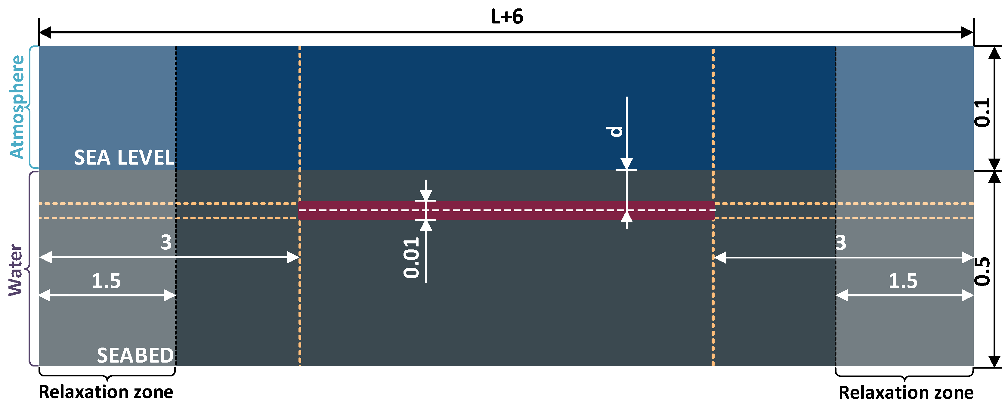
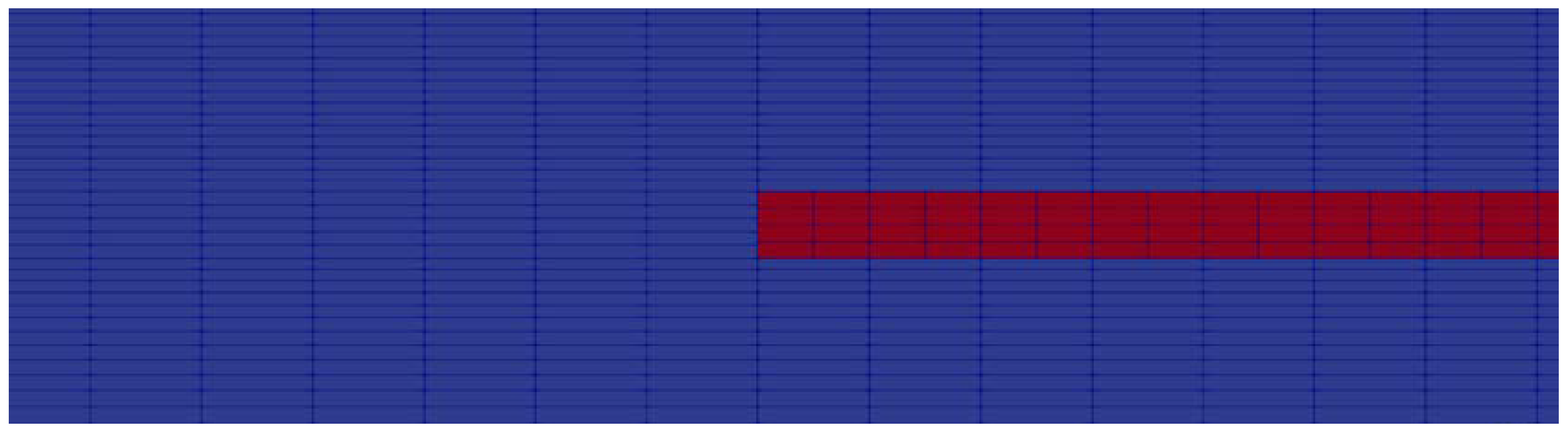
2.1.1. Computational Domain and Boundary Conditions

In an NWT, the boundary conditions include the inlet, outlet, wall, open boundary, etc. In the fluid subdomain, the top boundary applies the static pressure boundary to represent the atmospheric conditions, and the bottom is determined as the no-slip boundary to simulate the seabed. The left and right boundary are the inlet and outlet, respectively. The x-axis is parallel to the seabed and points from the inlet to outlet. The y-axis is positive upwards.

In the solid subdomain, except for the fixed boundary on the left, the rest of the boundary can move freely under external loads. The information exchange between the fluid subdomain and the solid subdomain also takes place within these boundaries.

The relaxation zone method is the main approach to generating and absorbing waves. Relaxation zones are provided on both the left and right sides of the NWT. This method introduces the spatial weighting factor χ and the equation is as follows:

$$\varphi =\chi {\varphi }_{\mathrm{computed}}+\left(1-\chi \right){\varphi }_{\mathrm{target}}$$

(1)

$\varphi$ can represent either the fluid velocity u or γ. γ represents the change in spatial variation of any fluid property, such as dynamic molecular viscosity, density and so on.

In the wave generation zone, χ gradually changes from 0 to 1 along the x-axis, and in the wave absorption zone, it gradually changes from 1 to 0. The above-mentioned wave generation and absorption are achieved by the open-source wave toolbox, waves2foam [30].

2.1.2. Computational Method

The finite volume method is a method used to discretise the computation domain into small cells in order to calculate and obtain the final numerical solution in the space domain. The finite volume method is widely used for solving fluids. Cardiff et al. developed a solver named solids4foam to solve the solid subdomain problem through FVM [29], which means that the calculation of FSI can be realised only by using FVM. Following the completion of the solution process, time and space will be discretised. In space, the computing domain is discretised into hexahedral elements in the form of mesh. In Openfoam, the front and back patches of a 2D model do not impose any boundary conditions, so they can be considered as “empty”. Therefore, hexahedral elements actually solve problems in 2D. In time, continuous time will be divided by a certain time step. The time step depends on the Courant number (Co) and it can be obtained using the following equation:

$$Co=\frac{u\Delta t}{\Delta x}<1$$

(2)

where Δt is the step size, u is the normal velocity, and Δx is the distance between the centres of two adjacent cells. Δt is set to 0.001 s in this NWT, and the Co will be significantly less than 1.

2.1.3. Fluid Solution

The Navier–Stokes (N-S) equations, based on conservation of mass and momentum, is the most commonly used governing equation in CFD. Because of different assumptions about fluids, the N-S equations are expressed differently depending on the situation.

$$\nabla \cdot \mathit{v}=0$$

(3)

$$\frac{\delta \left(\rho \mathit{v}\right)}{\delta t}+\nabla \cdot \left(\rho \mathit{vv}\right)=-\nabla P+\nabla \cdot \tau +\rho g$$

(4)

Incompressible, isothermal, Newtonian flow can be described by Equation (3) and Equation (4), where $\nabla$ is the Hamiltonian, v is the velocity vector, P is pressure, ρ is the density, and τ is the viscous stress in which μ is the dynamic viscosity, and g is the gravitational acceleration. τ can be described by the following equation:

$$\mathit{\tau }=\mu \left(\nabla \mathit{v}+\nabla {\mathit{v}}^T\right)$$

(5)

The interface between water and air is the free surface, and it can be captured by the VOF method. A passive scalar field α is introduced to determine whether a cell should be water or air by describing the volume fraction of air and water in the cell. When α = 1 for this cell, the fluid inside is water, and vice versa, it is air. When α is between 0 and 1, it means that the cell contains a mixture of water and air. The nature of the VOF method could cause the free surface to blur, which requires the mesh refinement near the free surface area; this could also be addressed by using isoAdvector or the ghost fluid method [33].

2.1.4. Structural Solution

The St. Venant–Kirchhoff constitutive material model is widely used in engineering, which can be combined with the law of momentum conservation to simulate the solid subdomain. The following description of the governing equations was originally developed by Tuković et al. [34].

Assuming that the solid is elastic and compressible, the law of conservation of momentum can be used to obtain the following equation:

$${\displaystyle \underset{V_0}{\int }{\rho }_{solid}\frac{\partial }{\partial t}}\left(\frac{\partial u}{\partial t}\right)dV={\displaystyle \underset{S_0}{\int }\mathit{n}\cdot \left(\sum \cdot {\mathit{F}}^T\right)}dS+{\displaystyle \underset{V_0}{\int }{\rho }_{solid}gdV}$$

(6)

ρ_solid is the density of solid material, u is the displacement vector, F = I + (∇u)T is the deformation gradient tensor, I is the second-order identity tensor, and Σ is the second Piola–Kirchhoff stress tensor, which is related to the Cauchy stress tensor σ by the following expression:

$$\sigma =\frac{1}{\det \mathit{F}}\mathit{F}\cdot \sum \cdot {\mathit{F}}^T$$

(7)

The stress/strain relationship is dictated as follows:

$$\sum =2GS+\Lambda \mathrm{tr}\left(S\right)I$$

(8)

where the Green–Lagrange strain tensor is as follows:

$$\mathit{S}=\frac{1}{2}\left[\nabla \mathit{u}+{\left(\nabla \mathit{u}\right)}^T+\nabla \mathit{u}\cdot {\left(\nabla \mathit{u}\right)}^T\right]$$

(9)

G and Λ are Lamé’s coefficients and they are related to Young’s modulus E and Poisson’s ratio v.

$$G=\frac{E}{2\left(1+v\right)}$$

(10)

$$\Lambda =\frac{vE}{\left(1+v\right)\left(1-2v\right)}$$

(11)

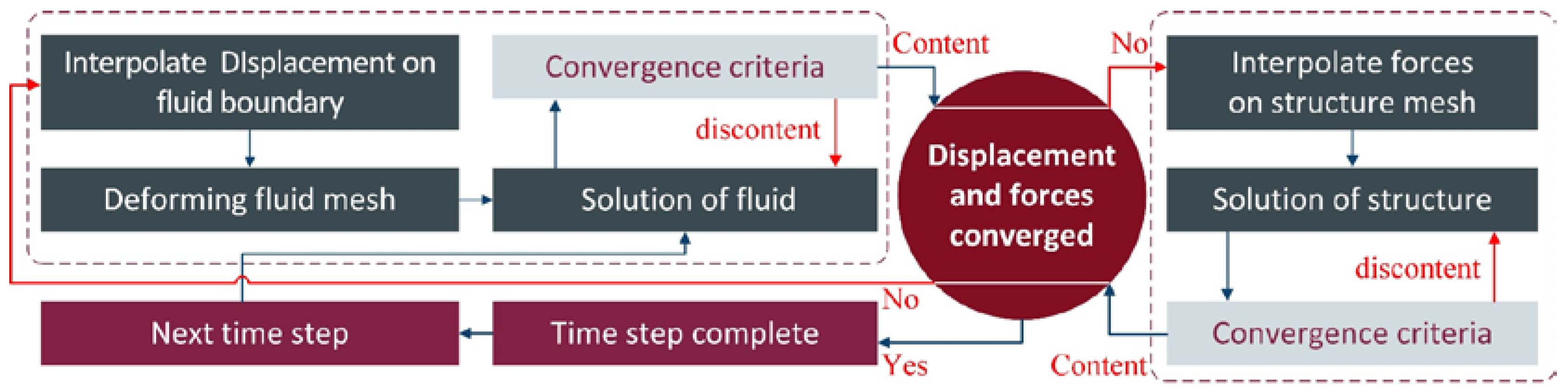
2.1.5. Fluid-Structure Interaction

Tuković et al. [34] proposed a partitioned FSI solver to couple the fluid and solid subdomains, which has been implemented in the OpenFOAM framework. Information about the fluid subdomains and solid subdomains can be extracted for the fluid-solid interfaces. First, the velocity and pressure of the fluid in the fluid subdomain are obtained, and the load is applied to the fluid-solid interface. Then, the displacement in the solid domain is solved, and the moving speed of the fluid-solid interface is obtained. When this process meets the convergence condition, it enters the next time step, and if not, the iteration continues. The whole calculation process is shown in Figure 3.

The matching of kinematic and dynamic conditions achieved in fluid-solid interfaces follows the following equations:

$$\left\{\begin{array}{l}{\mathit{v}}_{fluid}={\mathit{v}}_{solid}\hfill \\ {\mathit{u}}_{fluid}={\mathit{u}}_{solid}\hfill \\ n\cdot {\sigma }_{fluid}=n\cdot {\sigma }_{solid}\hfill \end{array}\right.$$

(12)

where v is the velocity vector, u is the displacement vector, n is the normal vector at the interface, and σ is the stress tensor.

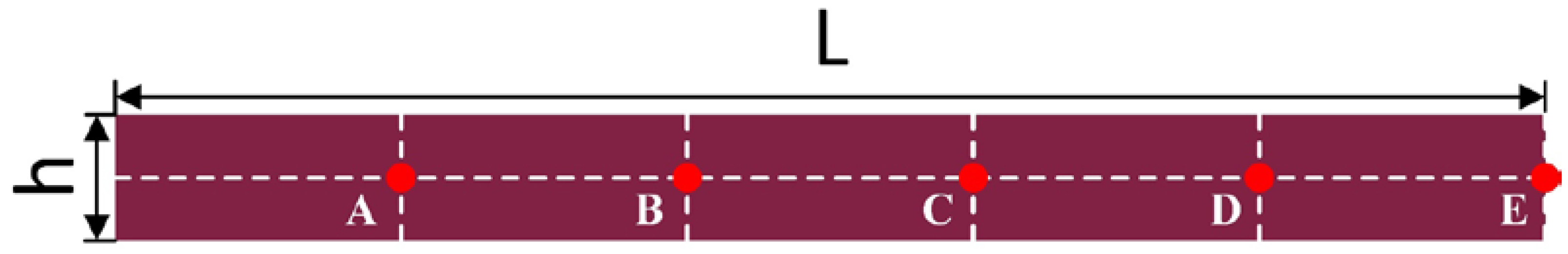
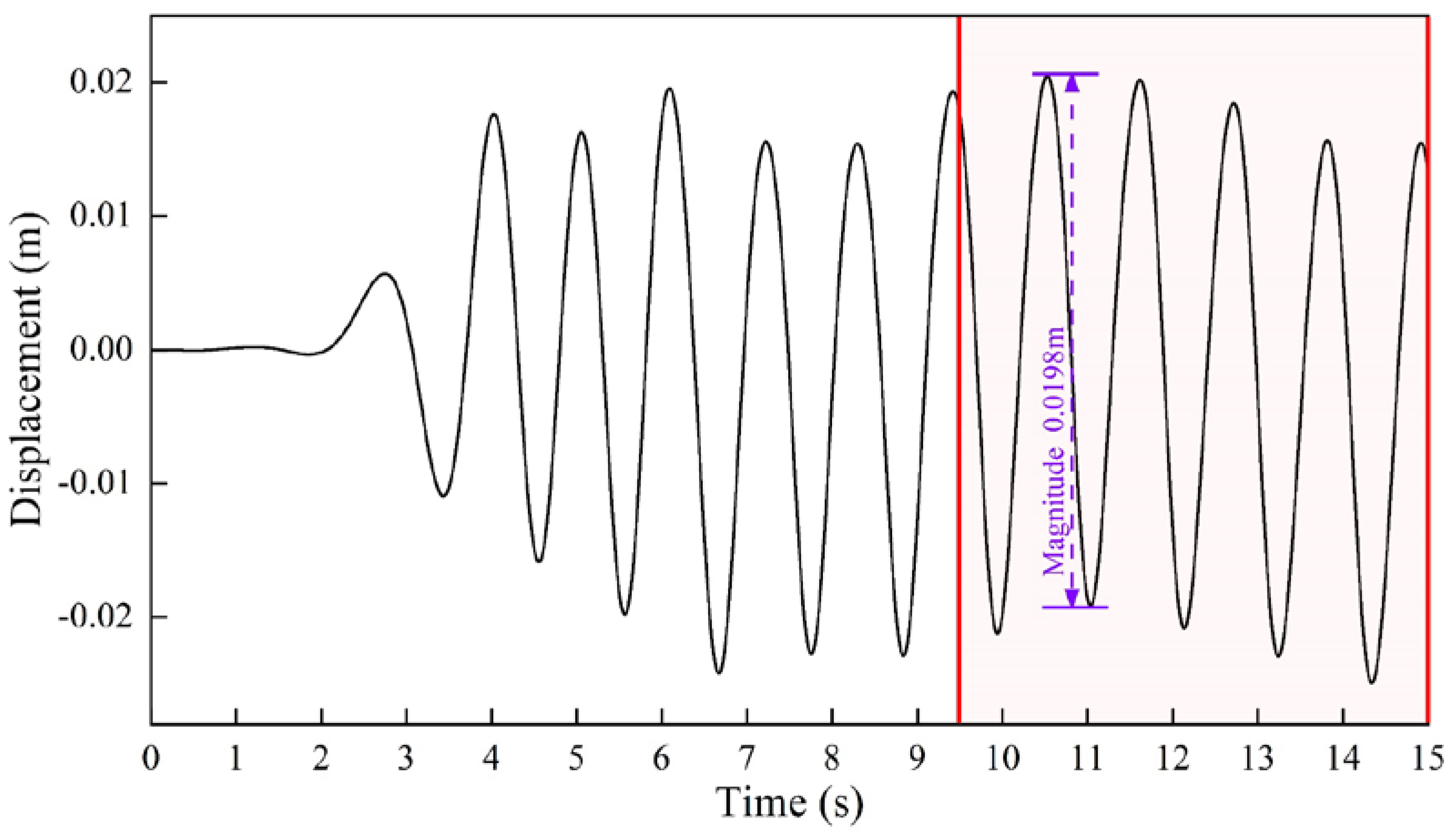
2.1.6. Data Acquisition and Processing

The displacement data were used to analyse the efficiency of the energy conversion, and the vertical displacement data of the flexible structure could be obtained with a probe in OpenFOAM. The probes are arranged at a distance of 0.2*L, 0.4*L, 0.6*L, 0.8*L and 1*L from the left edge of the flexible structure in the horizontal direction, and were deployed at the middle position of the flexible structure in the vertical direction. In Figure 4, the positions of the probes are marked with a red dot, where L and h represent the length and thickness of the flexible structure respectively.

In this research, the motion pattern of flexible structures in most cases are not sinusoidal. Therefore, it is necessary to obtain its amplitude in the frequency domain first by using the Fast Fourier Transform (FFT).

Figure 5 shows the displacement data obtained by the above probe located at point E (sea state: wave period 1.1 s, wave height 0.04 m, wave depth 1.5 m; deployment conditions of the flexible structure: L = 1.5112, d = 0.18) and the time required from wave action on the flexible structure to the full development of vibration is about 7 s. Therefore, it would be perfectly feasible to take the data after 9.5 s when analysing the amplitude.

In order to obtain the vibration amplitude of flexible structures more quickly and accurately, the Fast Fourier Transform (FFT) is applied to data processing. After FFT processing, the amplitude-frequency graph as shown in Figure 6 below can be obtained. Its X-coordinate has been normalised to the ratio of the wave frequency. From this figure, four peaks can be clearly discovered, which are roughly distributed in the position of f/f₀ of 0.33, 1 and 2. When f/f₀ is 1, the amplitude obtained by FFT is 0.0196 m, which is very close to the value of subtracting two peaks in the time domain, which also shows the reliability of this method.

The deformable WECs apply Dielectric Elastomer Generators (DEGs) to form a power take-off (PTO) system that generates electricity from structural deformations. In this work, the energy harnessed was calculated as the deformation energy per unit width of the device. The energy efficiency of the WEC was calculated by per unit width of harnessed energy divided by per unit width of wave energy, using the following equation:

$${\phi }_{FFT}=\frac{{\rho }_{WEC}{\displaystyle \sum _{i=1}^n{D_i}^2}}{{\rho }_{water}{a}^2}$$

(13)

The energy conversion efficiency of the device is obtained by averaging the φ_FFT obtained at each probe point. In addition, f/f₀ of 0.33 should not be involved in the calculation. This is an unstable vibration. When the calculation time is extended, the vibration at this frequency will disappear.

2.2. Verifications

In this section, the rationality and accuracy of the above model are verified following four steps: (a) determine the key parameters of the model; (b) certify fluid solution model simplification to laminar flow is reasonable; (c) determine if the mesh setup can ensure the accuracy of the wave generator and solid sub-domain displacement.

2.2.1. Fluid and Structural Parameters

Table 1. Basic parameters of wave.

Wave Type	Wave Period [s]	Height [m]	Wave Depth [m]	Wave Length [m]
Stokes Second	1.1	0.03 [m]	1.5	1.889

,

Table 2. Basic parameters of fluid.

Transport Model	Simulation Type	Density [kg/m3]	Kinematic Viscosity [m2/s]
Newtonian	Laminar	1000	1 × 10−6

and

Table 3. Basic parameters of solid.

Flexible Material Type	Density [kg/m3]	Young’s Modulus [Pa]	Poisson’s Ratio [-]
St. Venant–Kirchhoff Elastic	1000	5 × 107	0.3

show the parameters required for the calculation. The conditions of wave height and wavelength meet the requirements of Stokes second-order wave theory, and the values of H/gT² and d/gT² are 1.69 × 10⁻³ and 4.25 × 10⁻², respectively. The parameters of solids are similar to those of rubber because most of the current WECs based on flexible structures are made of rubber. The model-scale wave condition was chosen based on previous validation against experiments, including (a) wave transmission and reflection; (b) structural deformations in waves, which was reported in detail in [26]. However, the results will also be applicable on a larger scale following Froude scaling. Although the scaling will involve a mismatch in Reynolds numbers, the influence is expected to be minimal as inertial force is much more significant than viscous force in this application.

2.2.2. Laminar Flow

Compared with laminar flow, the turbulence model is suitable for cases where inertia is dominant in fluid flow. Due to the relatively complex computational mechanism of turbulence, many scholars have proposed a lot of different computational models. Therefore, for one new case, whether to adopt a turbulence model and what kind of turbulence model to adopt should be considered before running the simulation program.

The identification of which model should be used depends on a dimensionless quantity called the Reynolds number. The flexible structure is arranged in the ocean in a way similar to a swept plate. Generally, for the “swept plate” problem, when the Reynolds number is less than 5 × 10⁵, it is considered that there is no turbulent component in the fluid. In other words, the laminar flow model can be used in this model to reduce the computational cost. It has become common sense that the critical Reynolds number for laminar flow to become turbulent is between 3.2 × 10⁵ and 3 × 10⁶. The equation to calculate Reynolds number is as follows:

$$\mathrm{Re}=\frac{\rho vd}{\mu }$$

(14)

Re is the Reynolds number, ρ is the fluid density, v is the characteristic velocity, d is the characteristic length, and μ is the dynamic viscosity. In the case of the flexible structure, the characteristic length can be thought of as the length of the plate. Near the plate, the velocity of the fluid will not exceed 0.18 m/s, so the characteristic velocity can be thought of as 0.2 m/s. Even with relatively loose calculation parameters (Re = 2.7 × 10⁵), it is also difficult to reach the Reynolds number of 3.2 × 10⁵. Therefore, it can be considered that the laminar flow model is consistent with the actual situation. In addition, the Keulegan–Carpenter number is around 0.2, which is smaller than 1, indicating that the flow does not separate from the plate [36]; thus, no turbulence effect is expected in the present study. However, we note that this is an ideal case and turbulence can be ubiquitous in real oceans.

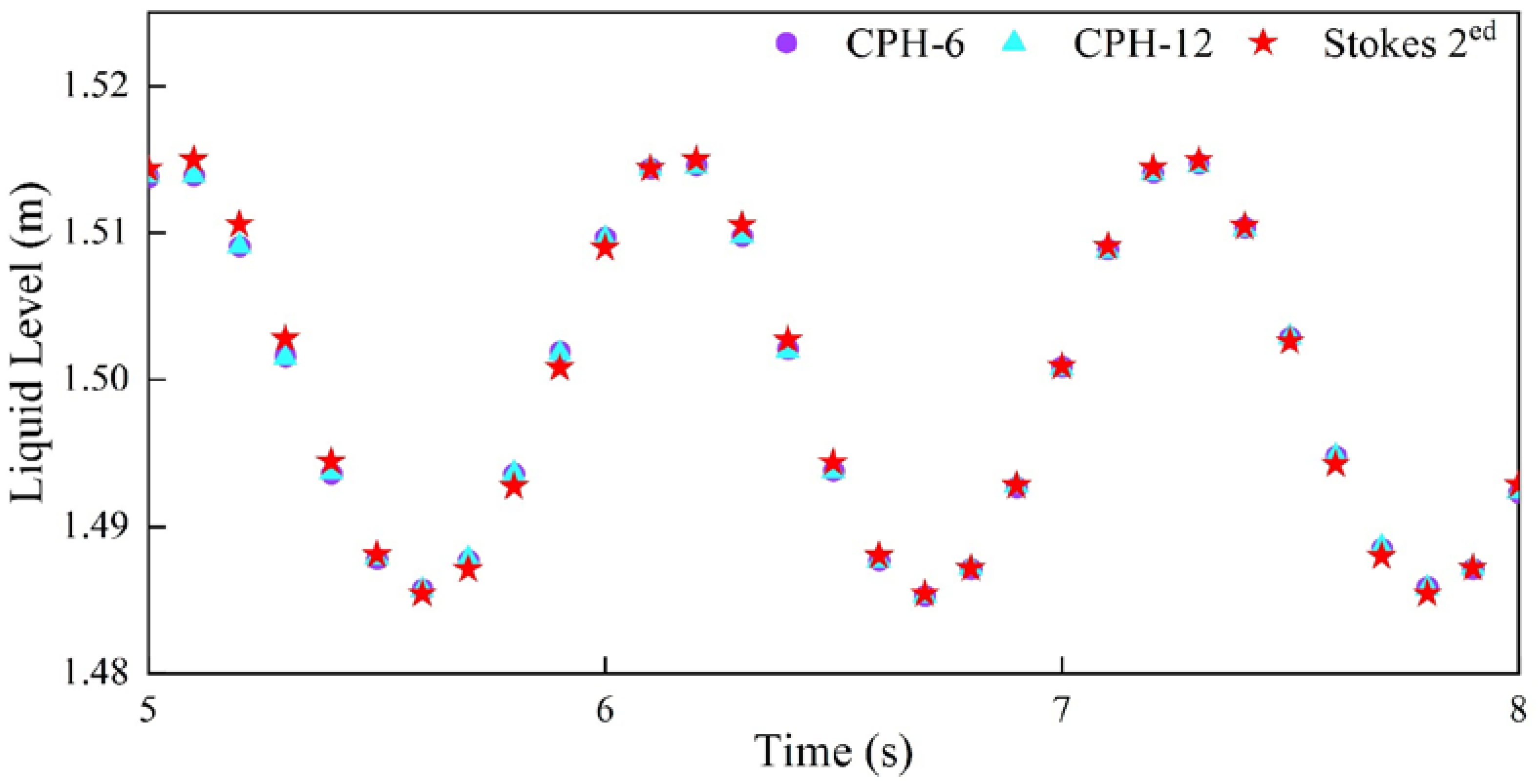
2.2.3. Mesh Convergence Study for Wave Modelling

The accuracy of wave modelling is closely related to the number of cells, and it is common practice to obtain the optimal number of cells by grid sensitivity analysis. Ref. [37] quantified the relationship between waves and cells using cells per wavelength (CPW) and cells per wave height (CPH). The discretisation error can be minimised when CPW and CPH reach 50 and 20, respectively.

In this study, CPW was set at 75, which was in line with the value recommended by the above literature. In order to explore the influence of different CPH on the calculation accuracy of liquid level height, the liquid level height located downstream was collected. The Root-Mean Squared Error (RMSE) calculated according to Equation (2) is shown in

Table 4. RMSE of different CPHs.

CPH	3	6	9	12
RMSE	7.12 × 10−7	7.26 × 10−7	6.97 × 10−7	7.14 × 10−7

. Increasing CPH from 3 to 12 had no significant impact on the calculation results. The results shown in Figure 7 coincide with the theoretical data when CPH is set to 6 and 12.

$$RMSE=\sqrt{\frac{{\displaystyle {\sum }_{i=1}^N{\left(x{\left(i\right)}_{predicted}-x{\left(i\right)}_{actual}\right)}^2}}{N}}$$

(15)

2.2.4. Mesh Convergence Study for Structural Modelling

The solid subdomains were spatially dispersed according to the four partition specifications of 38 × 3, 38 × 5, 76 × 5 and 76 × 8, respectively, in order to find the appropriate mesh parameters to avoid their great influence on the calculation results. In these four different specifications, the number of cells is 114,190,380 and 608. As shown in

Table 5. The energy conversion efficiency with different numbers of cells.

Number of Cells	114	190	380	608
Energy conversion efficiency	137.93%	138.49%	137.77%	138.52%

, there is little difference in the energy conversion efficiency obtained by different discrete settings, and the difference between the maximum and minimum values is only 0.75%.

Since the flow of liquid from the surface to the seabed tends to decrease gradually, the vertical mesh density can reduce the computational burden by decreasing gradually. The details of cells are shown in Figure 8.

3. Results and Discussion

Existing studies have shown that the efficiency of energy conversion is mainly related to the depth and length of the flexible structure [38]. In order to facilitate the development of the research, these two studied parameters were normalised. The length of the flexible structure and its depth in water are divided by the wavelength and height of the wave, respectively. The specific parameters are shown in

Table 6. Input conditions of simulation cases.

	L/λ = 0.2	L/λ = 0.25	L/λ = 0.3	L/λ = 0.4	L/λ = 0.5	L/λ = 0.6	L/λ = 0.65	L/λ = 0.7	L/λ = 0.75	L/λ = 0.8
d/H = 01	C020	C020.5	C021	C022	C023	C024	C024.5	C025	C025.5	C026
	L = 0.3778 d = 0.03	L = 0.4723 d = 0.03	L = 0.5667 d = 0.03	L = 0.7556 d = 0.03	L = 0.9445 d = 0.03	L = 1.1334 d = 0.03	L = 1.228 d = 0.03	L = 1.3223 d = 0.03	L = 1.4168 d = 0.03	L = 1.5112 d = 0.03
d/H = 02	C030	C030.5	C031	C032	C033	C034	C034.5	C035	C035.5	C036
	L = 0.3778 d = 0.06	L = 0.4723 d = 0.06	L = 0.5667 d = 0.06	L = 0.7556 d = 0.06	L = 0.9445 d = 0.06	L = 1.1334 d = 0.06	L = 1.228 d = 0.03	L = 1.3223 d = 0.06	L = 1.4168 d = 0.06	L = 1.5112 d = 0.06
d/H = 03	C040	C040.5	C041	C042	C043	C044	C044.5	C045	C045.5	C046
	L = 0.3778 d = 0.09	L = 0.4723 d = 0.09	L = 0.5667 d = 0.09	L = 0.7556 d = 0.09	L = 0.9445 d = 0.09	L = 1.1334 d = 0.09	L = 1.228 d = 0.03	L = 1.3223 d = 0.09	L = 1.4168 d = 0.09	L = 1.5112 d = 0.09
d/H = 04	C050	C050.5	C051	C052	C053	C054	C054.5	C055	C055.5	C056
	L = 0.3778 d = 0.12	L = 0.4723 d = 0.12	L = 0.5667 d = 0.12	L = 0.7556 d = 0.12	L = 0.9445 d = 0.12	L = 1.1334 d = 0.12	L = 1.228 d = 0.03	L = 1.3223 d = 0.12	L = 1.4168 d = 0.12	L = 1.5112 d = 0.12
d/H = 05	C060	C060.5	C061	C062	C063	C064	C064.5	C065	C065.5	C066
	L = 0.3778 d = 0.15	L = 0.4723 d = 0.15	L = 0.5667 d = 0.15	L = 0.7556 d = 0.15	L = 0.9445 d = 0.15	L = 1.1334 d = 0.15	L = 1.228 d = 0.03	L = 1.3223 d = 0.15	L = 1.4168 d = 0.15	L = 1.5112 d = 0.15
d/H = 06	C070	C070.5	C071	C072	C073	C074	C074.5	C075	C075.5	C076
	L = 0.3778 d = 0.18	L = 0.4723 d = 0.18	L = 0.5667 d = 0.18	L = 0.7556 d = 0.18	L = 0.9445 d = 0.18	L = 1.1334 d = 0.18	L = 1.228 d = 0.03	L = 1.3223 d = 0.18	L = 1.4168 d = 0.18	L = 1.5112 d = 0.18
d/H = 07	C080	C080.5	C081	C082	C083	C084	C084.5	C085	C085.5	C086
	L = 0.3778 d = 0.21	L = 0.4723 d = 0.21	L = 0.5667 d = 0.21	L = 0.7556 d = 0.21	L = 0.9445 d = 0.21	L = 1.1334 d = 0.21	L = 1.228 d = 0.03	L = 1.3223 d = 0.21	L = 1.4168 d = 0.21	L = 1.5112 d = 0.21
d/H = 08	C090	C090.5	C091	C092	C093	C094	C094.5	C095	C095.5	C096
	L = 0.3778 d = 0.24	L = 0.4723 d = 0.24	L = 0.5667 d = 0.24	L = 0.7556 d = 0.24	L = 0.9445 d = 0.24	L = 1.1334 d = 0.24	L = 1.228 d = 0.03	L = 1.3223 d = 0.24	L = 1.4168 d = 0.24	L = 1.5112 d = 0.24
d/H = 09	C100	C100.5	C101	C102	C103	C104	C104.5	C105	C105.5	C106
	L = 0.3778 d = 0.27	L = 0.4723 d = 0.27	L = 0.5667 d = 0.27	L = 0.7556 d = 0.27	L = 0.9445 d = 0.27	L = 1.1334 d = 0.27	L = 1.228 d = 0.03	L = 1.3223 d = 0.27	L = 1.4168 d = 0.27	L = 1.5112 d = 0.27
d/H = 10	C110	C110.5	C111	C112	C113	C114	C114.5	C115	C115.5	C116
	L = 0.3778 d = 0.30	L = 0.4723 d = 0.30	L = 0.5667 d = 0.30	L = 0.7556 d = 0.30	L = 0.9445 d = 0.30	L = 1.1334 d = 0.30	L = 1.228 d = 0.03	L = 1.3223 d = 0.30	L = 1.4168 d = 0.30	L = 1.5112 d = 0.30
d/H = 11	C120	C120.5	C121	C122	C123	C124	C124.5	C125	C125.5	C126
	L = 0.3778 d = 0.33	L = 0.4723 d = 0.33	L = 0.5667 d = 0.33	L = 0.7556 d = 0.33	L = 0.9445 d = 0.33	L = 1.1334 d = 0.33	L = 1.228 d = 0.03	L = 1.3223 d = 0.33	L = 1.4168 d = 0.33	L = 1.5112 d = 0.33
d/H = 12	C130	C130.5	C131	C132	C133	C134	C134.5	C135	C135.5	C136
	L = 0.3778 d = 0.36	L = 0.4723 d = 0.36	L = 0.5667 d = 0.36	L = 0.7556 d = 0.36	L = 0.9445 d = 0.36	L = 1.1334 d = 0.36	L = 1.228 d = 0.03	L = 1.3223 d = 0.36	L = 1.4168 d = 0.36	L = 1.5112 d = 0.36
d/H = 13	C140	C140.5	C141	C142	C143	C144	C144.5	C145	C145.5	C146
	L = 0.3778 d = 0.39	L = 0.4723 d = 0.39	L = 0.5667 d = 0.39	L = 0.7556 d = 0.39	L = 0.9445 d = 0.39	L = 1.1334 d = 0.39	L = 1.228 d = 0.09	L = 1.3223 d = 0.39	L = 1.4168 d = 0.39	L = 1.5112 d = 0.39

.

In addition to the above two factors, the Aspect Ratio (AR) may also have an impact on the energy conversion efficiency. AR refers to the ratio of L to h of the flexible structure. Since the length of the flexible structure is related to the wavelength, the optimal AR will be obtained by changing the thickness of the flexible structure. For ease of calculation, the flexible structure will be set to 1m in length and the d/H is set to 5.

Figure 9 provides an example of the WEC deformation for one wave period. It can be seen that the CFD and CSM solutions evolve together in the time domain, which demonstrates the fully coupled capability of the present model. It shows that the WEC deforms following the dominating wave shape and the end of the plate swings with the movement of the water. At the same time, because of the presence of WEC, the outgoing wave changes significantly compared with the incident wave.

It takes about 10 h to compute this example (13 wave cycles), using four performance cores of I7-12700K with a memory frequency of 5200 MHz. In particular, it should be pointed out that the model has very low memory requirements, and we only needed 4G RAM to meet the computing requirements.

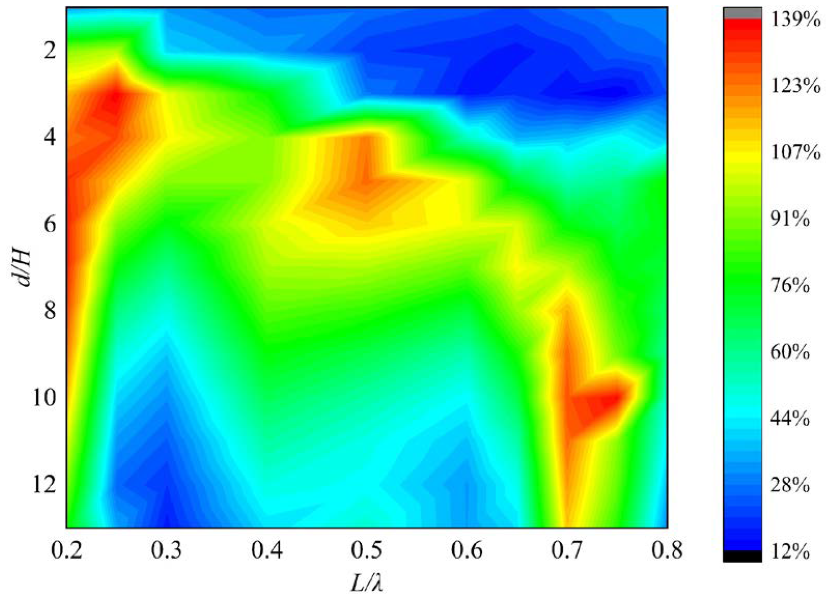
3.1. Effect of Deployment Depth and Length of Flexible Structure on Energy Conversion Efficiency

Figure 10 shows the energy conversion efficiency of flexible structures at different deployment depths and different lengths. It can be seen in the figure that when L/λ = 0.25 and d/H = 3, the energy conversion efficiency of the flexible structure reaches the highest value of 138.45%. Therefore, it can be considered that the best energy conversion efficiency can be obtained when the total length of the flexible structure is one-quarter of the wavelength and the deployment depth is three times the wave amplitude. When the relationship between the total length of the flexible structure and the wavelength is L/λ = 0.50 and L/λ = 0.75, the energy conversion efficiency of the device can also achieve a good effect (at d/H = 5 and d/A = 10, the energy conversion efficiency reaches 124.66% and 135.83%, respectively).

In terms of deployment depth, it seems that a larger L/λ requires a greater deployment depth. Moreover, in the case of insufficient deployment depth, the energy conversion efficiency will decline rapidly and significantly. This phenomenon is like a “wall”, and when the deployment depth passes this “wall”, the energy conversion efficiency will be significantly improved.

The interesting thing is, that when the value of L/λ is near 0.25, 0.5 and 0.75, the influence of the deployment depth of the flexible structure on the energy conversion efficiency will be weakened, which is very conducive to the deployment and application of this device, and it is a very challenging work to accurately control the deployment depth of the flexible structure.

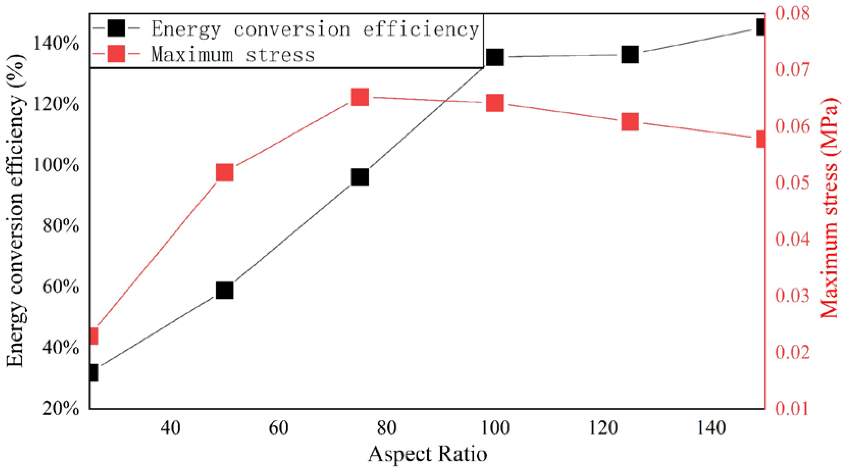
3.2. Relationship between AR and Energy Conversion Efficiency of Flexible Structure

Figure 11 shows the relationship between the AR and energy conversion efficiency under the sea state when the wave height, wave depth and period is 0.02 m, 1.5 m and 1.1 s. The flexible structure was deployed at a depth of 0.14 m below the water level, with a total length of 1m. The result shows that if the AR is too small, it will make the deformation of the flexible structure very difficult, and its motion pattern will be like that of a rigid body. As the AR decreases, the efficiency of energy conversion increases significantly. At the same time, with the increase in AR, the maximum stress of flexible structures increases first and then decreases slowly. The influence of the AR value on motion amplitude is also reflected in Figure 12, which is consistent with the conclusion of Figure 11. When the AR is 100 and 150, the limit range of motion is significantly greater than when the AR is 50. The motion amplitude of AR100 and AR150 also does not seem to differ much, which is in line with the content of the energy conversion efficiency in Figure 11.

The appearance of the maximum stress is related to the bending degree of the flexible structure, and the greater the bending degree, the greater the stress on the upper and lower planes. Figure 13 shows the stress distribution of a flexible structure under a wave load, when the flexible structure is subjected to its maximum stress at work.

These findings support the design and operation of deformable WECs by enabling the prediction of cyclic loading for fatigue life as well as extreme loading for ultimate strength; this can further inform the inspection schedule and maintenance strategies [39,40,41]. Thus, the present work may potentially improve the affordability and safety of the systems. When considering the energy efficiency and survivability of the device in relation to varying parameters such as device length and deployment depth, it should also be noted that costs are always an important trade-off. Therefore, the design should fully consider the deployment location’s wave conditions and choose the most cost-effective approach.

4. Conclusions

In this paper, a fully coupled CFD+CSM method was used to simulate the interaction between a deformable structure with nonlinear waves. On this basis, the energy conversion efficiency of a submerged deformable wave energy converter was studied with varying parameters of total length, deployment depth and AR. It was found that the total length of the flexible structure plays a crucial role in the energy conversion efficiency and when the total length of the flexible structure is 0.25, 0.5 and 0.75 times the wavelength, optimal energy conversion efficiency can be obtained. At the same time, the optimal deployment depth corresponding to these three lengths also increases with the structural length.

When AR increases, the plate structure is more prone to deformation, so the energy conversion efficiency shows a gradually increasing trend, and this trend is no longer obvious after reaching a certain limit. However, the improvement of energy conversion efficiency does not lead to a continuous increase in the load burden of flexible structures. Its maximum stress will reach a maximum value and then slowly decrease. The present work demonstrates a hydroelastic design methodology for a deformable wave energy converter, with a range of empirical rules that are useful for the industry.

Since the current CFD+CSM method has the computational power of two-way full coupling, the deformation of the structure and the change in the flow field can be clearly displayed, which can be used to assist the design work that is needed for marine structures with large deformations. Thus, this work tackles the technical challenge of modelling fully coupled fluid-structure interactions, which are essential for deformable WECs. Also, it facilitates the modelling of other offshore and coastal industries.

However, this model still has its limitations. The current simulation is performed in 2D, which excludes wave scattering near the geometry and potentially influences the energy efficiency in 3D. Advanced incorporation of DEGs as the PTO system should be developed in future work, e.g., mechanical damping; the present study also only simulated a single device and did not model the cases of array configurations, which are of interest [42,43,44]. Although regular wave conditions were used to establish relationships between energy efficiency and incident wave conditions, it is noted that realistic sea waves will be irregular and optimal performance might be achieved through a real-time PTO controlling strategy [45]. Based on the CFD+CSM approach, it is suggested in future work to explore the option of containing multiple materials in the CSM part [29]; the device geometry could be more complex and optimised in 3D [46], and mooring analysis could be added to enhance the practicalities [47].

References

1. Reguero, B.G.; Losada, I.J.; Méndez, F.J. A Global Wave Power Resource and Its Seasonal, Interannual and Long-Term Variability. Appl. Energy 2015, 148, 366–380. [Google Scholar] [CrossRef]
2. Mwasilu, F.; Jung, J. Potential for Power Generation from Ocean Wave Renewable Energy Source: A Comprehensive Review on State-of-the-art Technology and Future Prospects. IET Renew. Power Gener. 2019, 13, 363–375. [Google Scholar] [CrossRef]
3. Windt, C.; Davidson, J.; Ringwood, J.V. Numerical Analysis of the Hydrodynamic Scaling Effects for the Wavestar Wave Energy Converter. J. Fluids Struct. 2021, 105, 103328. [Google Scholar] [CrossRef]
4. Renzi, E.; Michele, S.; Zheng, S.; Jin, S.; Greaves, D. Niche Applications and Flexible Devices for Wave Energy Conversion: A Review. Energies 2021, 14, 6537. [Google Scholar] [CrossRef]
5. Collins, I.; Hossain, M.; Dettmer, W.; Masters, I. Flexible Membrane Structures for Wave Energy Harvesting: A Review of the Developments, Materials and Computational Modelling Approaches. Renew. Sustain. Energy Rev. 2021, 151, 111478. [Google Scholar] [CrossRef]
6. Farley, F.J.M.; Rainey, R.C.T.; Chaplin, J.R. Rubber Tubes in the Sea. Phil. Trans. R. Soc. A 2012, 370, 381–402. [Google Scholar] [CrossRef] [PubMed]
7. Alam, M.-R. A Flexible Seafloor Carpet for High-Performance Wave Energy Extraction. In Proceedings of the ASME 2012 31st International Conference on Ocean, Offshore and Arctic Engineering, Rio de Janeiro, Brazil, 1–6 July 2012; Volume 4: Offshore Geotechnics; Ronald W. Yeung Honoring Symposium on Offshore and Ship Hydrodynamics. American Society of Mechanical Engineers: New York, NY, USA; pp. 839–846. [Google Scholar]
8. Lehmann, M.; Elandt, R.; Pham, H.; Ghorbani, R.; Shakeri, M.; Alam, M.-R. An Artificial Seabed Carpet for Multidirectional and Broadband Wave Energy Extraction: Theory and Experiment. In Proceedings of the 10th European Wave and Tidal Energy Conference, Aalborg, Denmark, 2–5 September 2013. [Google Scholar]
9. Rosati Papini, G.P.; Moretti, G.; Vertechy, R.; Fontana, M. Control of an Oscillating Water Column Wave Energy Converter Based on Dielectric Elastomer Generator. Nonlinear. Dyn. 2018, 92, 181–202. [Google Scholar] [CrossRef]
10. Moretti, G.; Rosati Papini, G.P.; Daniele, L.; Forehand, D.; Ingram, D.; Vertechy, R.; Fontana, M. Modelling and Testing of a Wave Energy Converter Based on Dielectric Elastomer Generators. Proc. R. Soc. A 2019, 475, 20180566. [Google Scholar] [CrossRef] [PubMed]
11. Tarrant, K.; Meskell, C. Investigation on Parametrically Excited Motions of Point Absorbers in Regular Waves. Ocean Eng. 2016, 111, 67–81. [Google Scholar] [CrossRef]
12. Kornbluh, R.D.; Pelrine, R.; Prahlad, H.; Wong-Foy, A.; McCoy, B.; Kim, S.; Eckerle, J.; Low, T. From Boots to Buoys: Promises and Challenges of Dielectric Elastomer Energy Harvesting; Bar-Cohen, Y., Carpi, F., Eds.; Springer: San Diego, CA, USA, 2011; p. 797605. [Google Scholar]
13. Zheng, S.; Michele, S.; Liang, H.; Meylan, M.H.; Greaves, D. Wave Power Extraction from a Floating Elastic Disk-Shaped Wave Energy Converter. J. Fluid Mech. 2022, 948, A38. [Google Scholar] [CrossRef]
14. Michele, S.; Zheng, S.; Buriani, F.; Borthwick, A.G.L.; Greaves, D.M. Floating Hydroelastic Circular Plate in Regular and Irregular Waves. Eur. J. Mech. B/Fluids 2023, 99, 148–162. [Google Scholar] [CrossRef]
15. Zheng, S.; Phillips, J.W.; Hann, M.; Greaves, D. Mathematical Modelling of a Floating Clam-Type Wave Energy Converter. Renew. Energy 2023, 210, 280–294. [Google Scholar] [CrossRef]
16. Benites-Munoz, D.; Huang, L.; Anderlini, E.; Marín-Lopez, J.R.; Thomas, G. Hydrodynamic Modelling of An Oscillating Wave Surge Converter Including Power Take-Off. JMSE 2020, 8, 771. [Google Scholar] [CrossRef]
17. Cheng, Y.; Ji, C.; Zhai, G. Fully Nonlinear Analysis Incorporating Viscous Effects for Hydrodynamics of an Oscillating Wave Surge Converter with Nonlinear Power Take-off System. Energy 2019, 179, 1067–1081. [Google Scholar] [CrossRef]
18. López, M.; Taveira-Pinto, F.; Rosa-Santos, P. Numerical Modelling of the CECO Wave Energy Converter. Renew. Energy 2017, 113, 202–210. [Google Scholar] [CrossRef]
19. Penalba, M.; Kelly, T.; Ringwood, J.V. Using NEMOH for Modelling Wave Energy Converters: A Comparative Study with WAMIT. In Proceedings of the 12th European Wave and Tidal Energy Conference (EWTEC), Cork, Ireland, 27 August–1 September 2017. [Google Scholar]
20. Tan, M.; Cen, Y.; Yang, Y.; Liu, X.; Si, Y.; Qian, P.; Zhang, D. Power Absorption Modelling and Analysis of a Multi-axis Wave Energy Converter. IET Renew. Power Gen 2021, 15, 3368–3384. [Google Scholar] [CrossRef]
21. Penalba, M.; Giorgi, G.; Ringwood, J.V. Mathematical Modelling of Wave Energy Converters: A Review of Nonlinear Approaches. Renew. Sustain. Energy Rev. 2017, 78, 1188–1207. [Google Scholar] [CrossRef]
22. Finnegan, W.; Rosa-Santos, P.; Taveira-Pinto, F.; Goggins, J. Development of a Numerical Model of the CECO Wave Energy Converter Using Computational Fluid Dynamics. Ocean. Eng. 2021, 219, 108416. [Google Scholar] [CrossRef]
23. Chen, W.; Dolguntseva, I.; Savin, A.; Zhang, Y.; Li, W.; Svensson, O.; Leijon, M. Numerical Modelling of a Point-Absorbing Wave Energy Converter in Irregular and Extreme Waves. Appl. Ocean. Res. 2017, 63, 90–105. [Google Scholar] [CrossRef]
24. Yeylaghi, S.; Moa, B.; Oshkai, P.; Buckham, B.; Crawford, C. ISPH Modelling of an Oscillating Wave Surge Converter Using an OpenMP-Based Parallel Approach. J. Ocean Eng. Mar. Energy 2016, 2, 301–312. [Google Scholar] [CrossRef]
25. Huang, L.; Ren, K.; Li, M.; Tuković, Ž.; Cardiff, P.; Thomas, G. Fluid-Structure Interaction of a Large Ice Sheet in Waves. Ocean Eng. 2019, 182, 102–111. [Google Scholar] [CrossRef]
26. Huang, L.; Li, Y. Design of the Submerged Horizontal Plate Breakwater Using a Fully Coupled Hydroelastic Approach. Comput. Aided Civ. Eng. 2022, 37, 915–932. [Google Scholar] [CrossRef]
27. Hu, Z.; Huang, L.; Li, Y. Fully-Coupled Hydroelastic Modeling of a Deformable Wall in Waves. Coast. Eng. 2023, 179, 104245. [Google Scholar] [CrossRef]
28. Jasak, H.; Jemcov, A.; Tukovic, Z. OpenFOAM: A C++ Library for Complex Physics Simulations. In Proceedings of the International Workshop on Coupled Methods in Numerical Dynamics IUC, Dubrovnik, Croatia, 19–21 September 2007. [Google Scholar]
29. Cardiff, P.; Karač, A.; De Jaeger, P.; Jasak, H.; Nagy, J.; Ivanković, A.; Tuković, Ž. An Open-Source Finite Volume Toolbox for Solid Mechanics and Fluid-Solid Interaction Simulations. arXiv 2018, arXiv:1808.10736. [Google Scholar]
30. Jacobsen, N.G.; Fuhrman, D.R.; Fredsøe, J. A Wave Generation Toolbox for the Open-Source CFD Library: OpenFoam®: WAVE GENERATION TOOLBOX. Int. J. Numer. Meth. Fluids 2012, 70, 1073–1088. [Google Scholar] [CrossRef]
31. Hirt, C.W.; Nichols, B.D. Volume of Fluid (VOF) Method for the Dynamics of Free Boundaries. J. Comput. Phys. 1981, 39, 201–225. [Google Scholar] [CrossRef]
32. Windt, C. High-Fidelity Numerical Modelling of Ocean Wave Energy Systems_ A Review of Computational Fluid Dynamics-Based Numerical Wave Tanks. Renew. Sustain. Energy Rev. 2018, 93, 610–630. [Google Scholar] [CrossRef]
33. Huang, L.; Li, Y.; Benites, D.; Windt, C.; Feichtner, A.; Tavakoli, S.; Davidson, J.; Paredes, R.; Quintuna, T.; Ransley, E.; et al. A review on the modelling of wave-structure interactions based on OpenFOAM. OpenFOAM J. 2022, 2, 116–142. [Google Scholar]
34. Tuković, Ž.; Karač, A.; Cardiff, P.; Jasak, H.; Ivanković, A. OpenFOAM Finite Volume Solver for Fluid-Solid Interaction. Trans. FAMENA 2018, 42, 1–31. [Google Scholar] [CrossRef]
35. Benra, F.-K.; Dohmen, H.J.; Pei, J.; Schuster, S.; Wan, B. A Comparison of One-Way and Two-Way Coupling Methods for Numerical Analysis of Fluid-Structure Interactions. J. Appl. Math. 2011, 2011, 1–16. [Google Scholar] [CrossRef]
36. Sumer, B.M.; Fredsøe, J. Hydrodynamics around Cylindrical Strucures; World Scientific: Singapore, 2006; Volume 26. [Google Scholar]
37. Connell, K.O.; Cashman, A. Development of a Numerical Wave Tank with Reduced Discretization Error. In Proceedings of the 2016 International Conference on Electrical, Electronics, and Optimization Techniques (ICEEOT), Chennai, India, 3–5 March 2016; IEEE: Chennai, India, 2016; pp. 3008–3012. [Google Scholar]
38. Huang, L.; Hu, Z.; Li, Y.; Thomas, G. Fully-Coupled CFD+CSM Analysis on an Elastic Floating/Submerged Plate for Wave Energy Harvest. In Proceedings of the 9th International Conference on Hydroelasticity in Marine Technology, Rome, Italy, 10–13 July 2022. [Google Scholar]
39. Cerik, B.C.; Choung, J. Fracture Prediction of Steel-Plated Structures under Low-Velocity Impact. JMSE 2023, 11, 699. [Google Scholar] [CrossRef]
40. Ringsberg, J. Life Prediction of Rolling Contact Fatigue Crack Initiation. Int. J. Fatigue 2001, 23, 575–586. [Google Scholar] [CrossRef]
41. Ringsberg, J. Prediction of Fatigue Crack Initiation for Rolling Contact Fatigue. Int. J. Fatigue 2000, 22, 205–215. [Google Scholar] [CrossRef]
42. Benites-Munoz, D.; Huang, L.; Thomas, G. Optimal Array Arrangement of Oscillating Wave Surge Converters: An Analysis Based on Three Devices. Renew. Energy 2024, 222, 119825. [Google Scholar] [CrossRef]
43. Zheng, S.; Michele, S.; Liang, H.; Iglesias, G.; Greaves, D. Wave Power Extraction from a Wave Farm of Tubular Structure Integrated Oscillating Water Columns. Renew. Energy 2024, 225, 120263. [Google Scholar] [CrossRef]
44. Wei, Y.; Wang, C.; Chen, W.; Huang, L. Array analysis on a seawall-type of deformable wave energy converters. Renew. Energy 2024, 225, 120344. [Google Scholar] [CrossRef]
45. Anderlini, E. Control of wave energy converters using machine learning strategies. PhD Thesis, University of Edinburgh, Edinburgh, UK, 2017. [Google Scholar]
46. Edwards, E.C.; Yue, D.K.P. Optimisation of the geometry of axisymmetric point-absorber wave energy converters. J. Fluid Mech. 2022, 933, A1. [Google Scholar] [CrossRef]
47. Wei, Y.; Yu, S.; Jin, P.; Huang, L.; Elsherbiny, K.; Tezdogan, T. Coupled analysis between catenary mooring and VLFS with structural hydroelasticity in waves. Mar. Struct. 2024, 93, 103516. [Google Scholar] [CrossRef]
Figure 1. Examples of flexible WECs. (a), reprinted from [4]. (bd), reprinted from [5].
Oceans 05 00014 g001
Figure 2. Schematic of the case: a flat flexible structure arranged under water is subjected to an incident wave and produces elastic deformation. L and d are the total length and deployment depth of the device (All units of length are meters).
Oceans 05 00014 g002
Figure 3. Solution algorithm for strong two-way coupling (reset the figure in [35]).
Oceans 05 00014 g003
Figure 4. The location of displacement probes (A, B, C, D, E).
Oceans 05 00014 g004
Figure 5. Example of vertical vibration displacement at a point of the flexible structure (The data in the red box is used for analysis).
Oceans 05 00014 g005
Figure 6. An example of FFT processing to show the displacement amplitude at different f/f0.
Oceans 05 00014 g006
Figure 7. Liquid level data at CPH 6 and 12 (compared with data obtained through Stokes second-order wave theory).
Oceans 05 00014 g007
Figure 8. Combined fluid and solid mesh (red part for solid subdomain and blue part for fluid subdomain).
Oceans 05 00014 g008
Figure 9. Periodic interaction between the flexible WEC and incoming waves (C063). The applied wave condition in this figure is T = 1.1 s and H = 0.03 m. In the subfigures, the water phase is beneath the free surface in red, while the air phase is above the free surface in blue.
Oceans 05 00014 g009aOceans 05 00014 g009b
Figure 10. Heat map of energy conversion efficiency.
Oceans 05 00014 g010
Figure 11. The relationship between conversion efficiency, maximum stress and AR.
Oceans 05 00014 g011
Figure 12. Upward limit (solid line) and downward limit (dash line) of the flexible structure’s deformations with different ARs.
Oceans 05 00014 g012
Figure 13. Stress distribution of flexible structures under wave load (t = nT + 7/10T).
Oceans 05 00014 g013