Abstract
Design of new materials is quite a difficult task owing to various time and length scales and affiliated uncertainties. The major challenge is to include all these in a conventional model. Hyperparameter models in machine learning can be used to overcome these issues. In this paper, an artificial neural network (ANN) model is developed to estimate the effective elastic parameters of unidirectional fiber reinforced composites using representative volume elements (RVE) considering uncertainty in the fiber diameter. The diameter probability distribution is constructed from the acquired gray images by employing image processing operations. The generalized Polynomial Chaos (gPC) expansion is then used to represent the distribution as a random input parameter for finite element analysis, from where the effective parameters are realized. Similarly, the outputs of the FE model, i.e., elastic parameters, are approximated by gPC expansions having unknown deterministic coefficients and random orthogonal Hermite polynomials. A set of collocation points are generated from roots of the random polynomials; from there, the unknown coefficients are estimated. The realization samples are utilized to train an ANN algorithm based on supervised deep learning. The developed ANN model is later tested and validated for a new sample set of data. It is shown that the ANN model with few hidden layers and neurons has a high accuracy for estimation of the elastic parameters directly from the information on the distribution of fiber diameters.
1. Introduction
Under many situations, the conventional modeling and simulations for calculation of state parameters break down due to material being nonlinear, multiscale, unknown, and high dimensional, as well as uncertainty, etc. The estimation of such parameters for the heterogeneous materials based on multiscale micromechanics models have been widely explored in past decades [1], analytically and numerically [2,3,4,5]. The experimental determination of such parameters is, however, a very expensive process. Furthermore, deterministic analysis leads to nominal design due to the inherent randomness in constitutive components. Uncertainty in material and geometrical parameters can be captured very well [6] in Monte Carlo based finite element (FE) analysis but applicability in the design phase is limited by the computational time. The major challenge is to include all these in conventional models. On the other hand, the availability of large data on such material motivates to develop databased numerical models from which the parameters can be estimated.
Designing of new materials to achieve tunable properties is an important task in engineering. The process is, however, quite difficult, and the modeling process faces an inverse problem. In contrast to the forward modeling problem, here, the structure of material and combination ratios are unknown. In many cases, any explicit knowledge about the physical behavior of such parameters is unavailable or limited. Consequently, various models at different length and time scales have to be investigated to achieve the desired properties. Furthermore, it is mandatory to include the details of each scale, including uncertainties between scales. Involving all these in a physics-based conventional modeling tool such as the FE method is not possible, or at least very difficult for implementation. Machine learning (ML) based algorithms provide such facilities where the available data or information on the material is fed to a hyperparameter computer algorithm to detect the governing rules or relationships between the data. The rules are later used for constructing a prediction model. Such nonconventional modeling has a great benefit when one deals with uncertainty in the state variables. The application of ML, particularly Artificial Neural Networks (ANN), in composite materials has been reported in the past few years [7,8,9,10,11]. In most of these studies, the impact of uncertainties in the microstructure and material properties have been ignored.
In this paper a supervised Deep Learning (DL) model is developed to predict the elastic parameters of unidirectional (UD) fiber composites considering uncertainty in the fiber geometrical parameters. Image processing techniques [12] are used to realize the probability distribution of the fiber diameter. The distribution is then approximated by the generalized Polynomial Chaos (gPC) expansion to be used as input for FE simulation. The FE analysis is carried out using RVE to realize the elastic parameters employing micromechanical models. The realizations are utilized to construct an ANN predictive model having a predefined architecture. The ANN model is trained on a random set of the available data based on the supervised machine learning algorithms. The prediction model is then validated on a set of new data generated from FE simulations for new a probability distribution of fiber diameter.
This paper is organized as follows: in the next section, we present the basic theory of micromechanics for parameter estimation. The theory of machine learning for micromechanics under uncertainty is presented in Section 3. Numerical results are given in Section 4 and Section 5 discusses the conclusions.
2. Micromechanics Based Estimation of Elastic Parameters
In this section, the classical computational micromechanics is employed for estimation of elastic parameters of UD fiber composites. The procedure deals with strictly methods, i.e., empirical adjusting factors are not required [13]. It is assumed that materials have isotropic cylindrical infinite fibers embedded in an elastic matrix, see Figure 1a. Furthermore, the Ruess model (constant strain), cf. Figure 1b, is used to estimated the modulus , , the shear modulus and Poisson’s ratio .
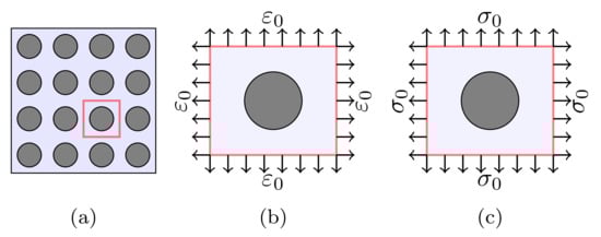
Figure 1.
(a) Cross section of composite material. Representing the RVE based on (b) Vogit and (c) Reuss models.
Assuming the orthotropic material properties at the mesoscale (lamina), the random stiffness tensor is estimated as
in which and are row and column vectors, respectively, and denotes vector of n random dimensions of the random space representing material and geometry uncertainties. To evaluate the elastic tensor, the RVE is subjected to a constant strain at all its boundary conditions, i.e.,
where and are the values of at and , respectively. This yields in the state of uncertain strain at each point inside the RVE having volume V, represented as
This results in state of stress in the RVE. By setting a unit value for , one can calculate the components of the elastic tensor as
In terms of FE calculations, the uncertain components of are estimated by averaging the element stress field in Equation (4) over the element volume given by
where denotes the average stress, is the element volume and represents the average elemental stress. Once the components of tensor are estimated, the uncertain elastic parameters are calculated, e.g., for
The random vector , in this paper, is limited only to geometric uncertainty in the diameters of fibers. In FE simulations, it is represented as an input random variable and approximated by the generalized Polynomial Chaos (gPC) expansion [14]. In analogy to this, the uncertain elastic parameters are represented as gPC expansions having unknown coefficients and a random orthogonal basis. Here, in this paper, orthogonal Hermite polynomials are used as the expansion basis. The unknown coefficients are then calculated on a set of elastic parameters generated on sample collocation points, cf. [6].
3. Deep Learning for Micromechanics under Uncertainty
In this section, the supervised DL method is adopted for estimation of uncertain elastic parameters of lamina considering randomness in fiber diameters. It was assumed that the UD composite material has cylindrical fibers with random diameters and infinite lengths embedded in an elastic matrix. Samples of RVE cells [15] were considered with the fiber diameter as the random variable. The finite element model of each RVE was then developed to estimate the vector of macro-scale elastic parameters represented as . The DL process begins with a set of input data collection on the assigned target output, , approximated by a functional , in the form of
The row vector denotes unknown adaptive parameters associated with each hidden layer in the artificial neural network (ANN), cf. Figure 2.
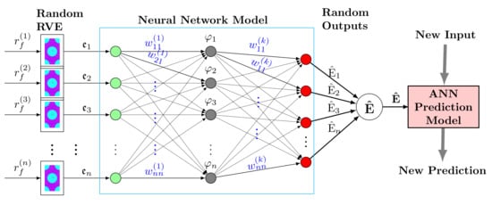
Figure 2.
Feedforward ANN for predicting of elastic parameters from microcells with uncertain fiber diameters, .
Generally, the basis is a set of nonlinear orthogonal functions. The activation function f is considered as the identity in the case of parameter estimation. The goal of this is to develop a model by adjusting the basis functions depending on the set of initial parameters which have to be updated during training. The process requiring the most effort in the DL process during this step is the estimation of the parameters. Furthermore, the input data have to be preprocessed, including data labeling [16] and dimension reduction methods such as Singular Value Decomposition (SVD) [17] and Dynamic Mode Decomposition (DMD) [18]. The refined data are then used for the featurization step where the most informative and nonredundant features of the data, e.g., statistical moments, are extracted. This facilitates the subsequent learning step in which the data are initially split into training and testing sets. The training data set is employed to train the algorithm via a supervised learning method to estimate the unknown parameters using an optimization method such as gradient descent or stochastic gradient descent [19]. A cost function is usually defined based on the least squares to estimate the parameters, i.e.,
with as the regularization factor. The second term, known as the penalty term, is often used to control the over-fitting phenomenon in order to discourage the coefficients from reaching large values, cf. [20]. The training step comprises estimation of the parameter set via an optimization process by minimizing the cost function. The data samples, here a set of elastic parameters, are then split into two sets: training and testing sets. As a rule of thumb, this can be and for training and testing sets, respectively. The training set was used to estimate the unknown parameter set . A common approach is to employ the gradient descent to update the parameters at each step k in the negative direction of gradient, that is
The parameter represents a positive step size, known as the learning rate. Both training rate and the descent direction are determined at each step, so that the sequence converges to the local or global minimum of the cost function. The step size was decreased after each successful step and increased only when a tentative step would increase the cost function. In this way, one can make sure that the cost function is always reduced at each iteration of the algorithm. The estimated error was then propagated to the ANN back to update the parameters. As the cost function has the form of a sum of squares, the gradient can be computed as
in which is the Jacobian matrix that contains first derivatives of the network errors with respect to the weights, and is the vector of network errors. The Jacobian matrix is computed through a standard backpropagation technique [21]. This has a major advantage over computing the Hessian matrix owing the fact that information on the second derivatives is not required.
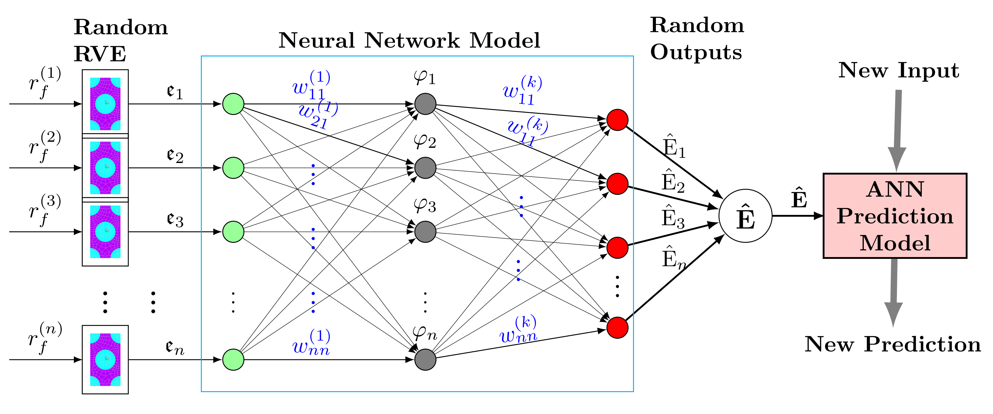
The major goal of using the above DL model is to achieve generalization by developing an accurate prediction model for new data. Once the parameter set is estimated, the developed model in Equation (7) can be used to predict the elastic parameters of lamina by introducing the fiber diameter as new input data. This has been demonstrated in Figure 3.
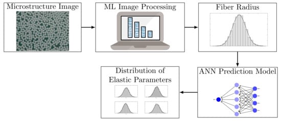
Figure 3.
DL based prediction model for estimating the elastic parameters of the composite.
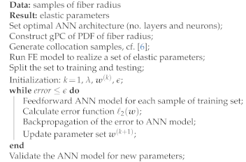
As shown, high-resolution digitally acquired micrographs of microstructure images can be used to extract the probability distribution of fibers [22,23]. One can obtain the elastic parameters by considering a separate data test comprising a set of fiber diameters using image processing [24]. As the predictive model estimates samples of elastic parameters, the statistical properties of the estimated parameters, e.g., probability density function (PDF), can then be evaluated using any post-processing analysis. Here, in this paper, the statistical moments of the estimated data are used to construct the gPC, from which the PDF of parameters are evaluated [25]. A summary of the numerical procedure is given in Algorithm 1.
| Algorithm 1:Supervised ANN algorithm for estimation of elastic parameters. |
 |
4. Case Study
In this section, the above procedure is applied to estimate the elastic parameters of lamina under uncertainty in the fiber diameter. The material properties of the considered unidirectional composite with isotropic fibers and matrix are given in Table 1.

Table 1.
Elastic properties of matrix and transverse isotropic fiber for the training phase of the developed ANN.
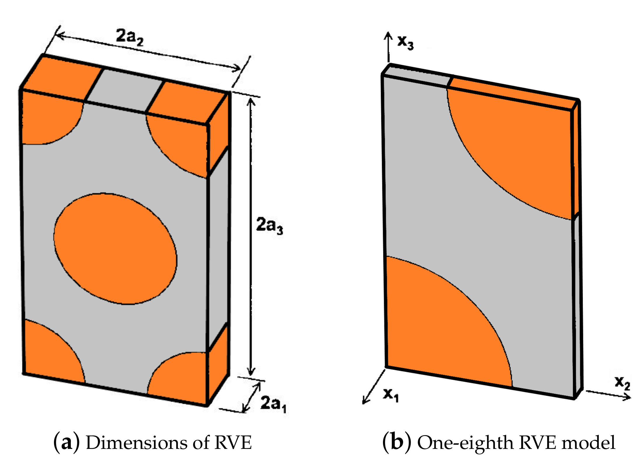
Note that in terms of engineering constants for the 3D orthotropic RVE and taking into account that the directions and are indistinguishable, the transversely isotropic material is assumed, i.e., , , and . The full size RVE used for FE simulations exhibiting nominal dimensions of is shown in Figure 4a, whereas an one-eighth 3D model of the RVE is employed in the numerical simulation due to the symmetry, cd. (Figure 4b).

Figure 4.
The implemented RVE with dimensions in the FE simulation.
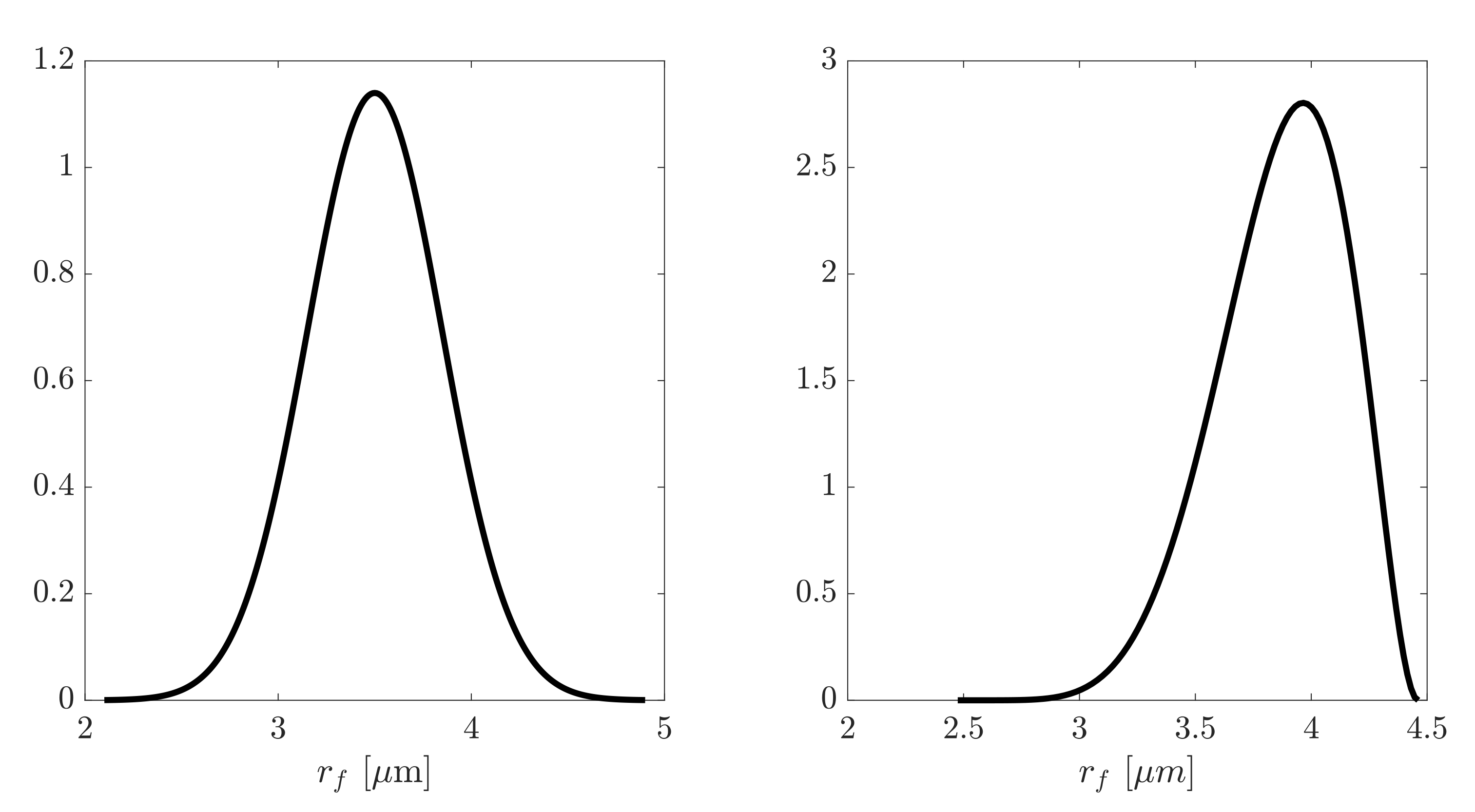
The total volume of the RVE was fixed as the fiber radius varied. The model was set up with the fiber along the axis and symmetry boundary conditions were applied on the planes , and , while a uniform displacement was applied on the plane . It was assumed that the fiber radius can be represented by the normal distribution, i.e., . The radius of fiber used for the ANN training was considered as a random variable having the mean value of m with the standard deviation of m. The predicted ANN model was then validated by using new data generated for the PDF shown on the right side of Figure 5.
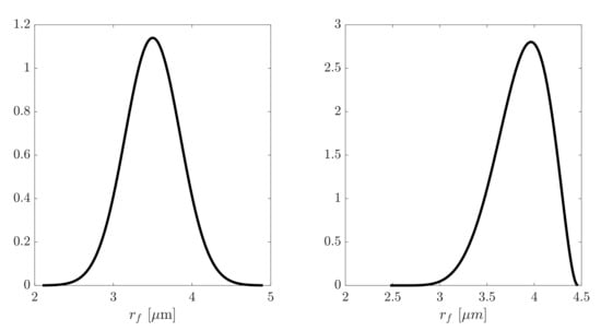
Figure 5.
PDF of the random fiber radius for training (left) and validation (right) of the ANN.
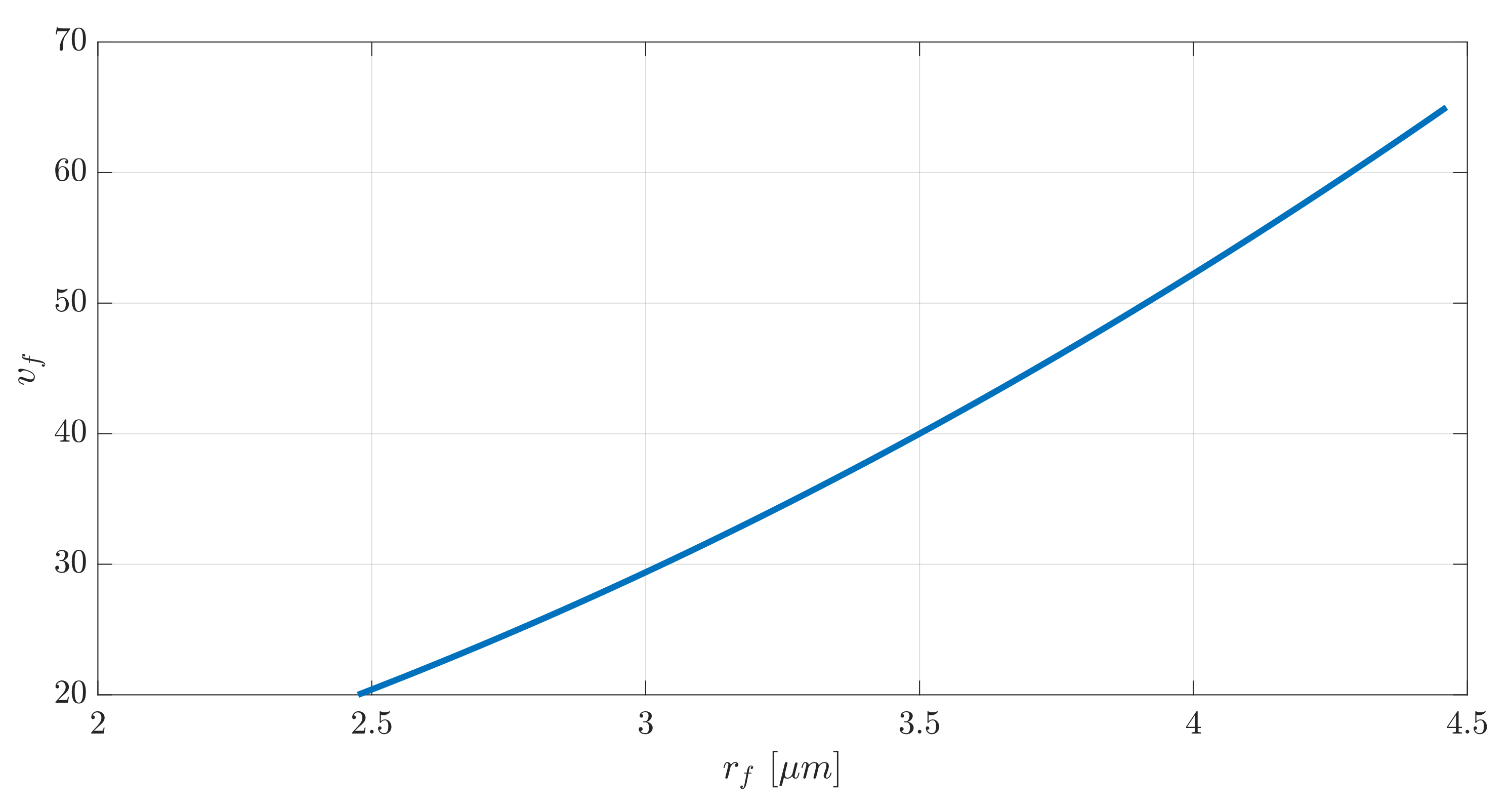
Due to the randomness in the fiber diameters, the volume fraction is no longer a constant value. Assuming that each fiber has a circular cross-sectional with the same diameter, this is shown in Figure 6.

Figure 6.
Relation between the volume fraction, , and the fiber radius, .
As demonstrated, this relationship is not linear.
In order to determine the components of the elastic matrix and, accordingly, the elastic parameters of lamina, a unit strain was applied to the unit cell in all directions in sequence while other components of strains were set to zero. This produces a uniform deformation corresponding to each boundary condition. A classical FE simulation using solid element was employed to estimate the elastic parameters of the lamina, i.e., and Poisson’s ratio . Two elements per thickness of the RVE was set and the static analysis was performed. A set of 500 samples for each parameter were collected using the constructed gPC expansions. The data were then preprocessed to detect any outlier due to truncated numerical error. This is due to the fact that any outlier may affect the optimization process, particularly when one uses the gradient descent method.
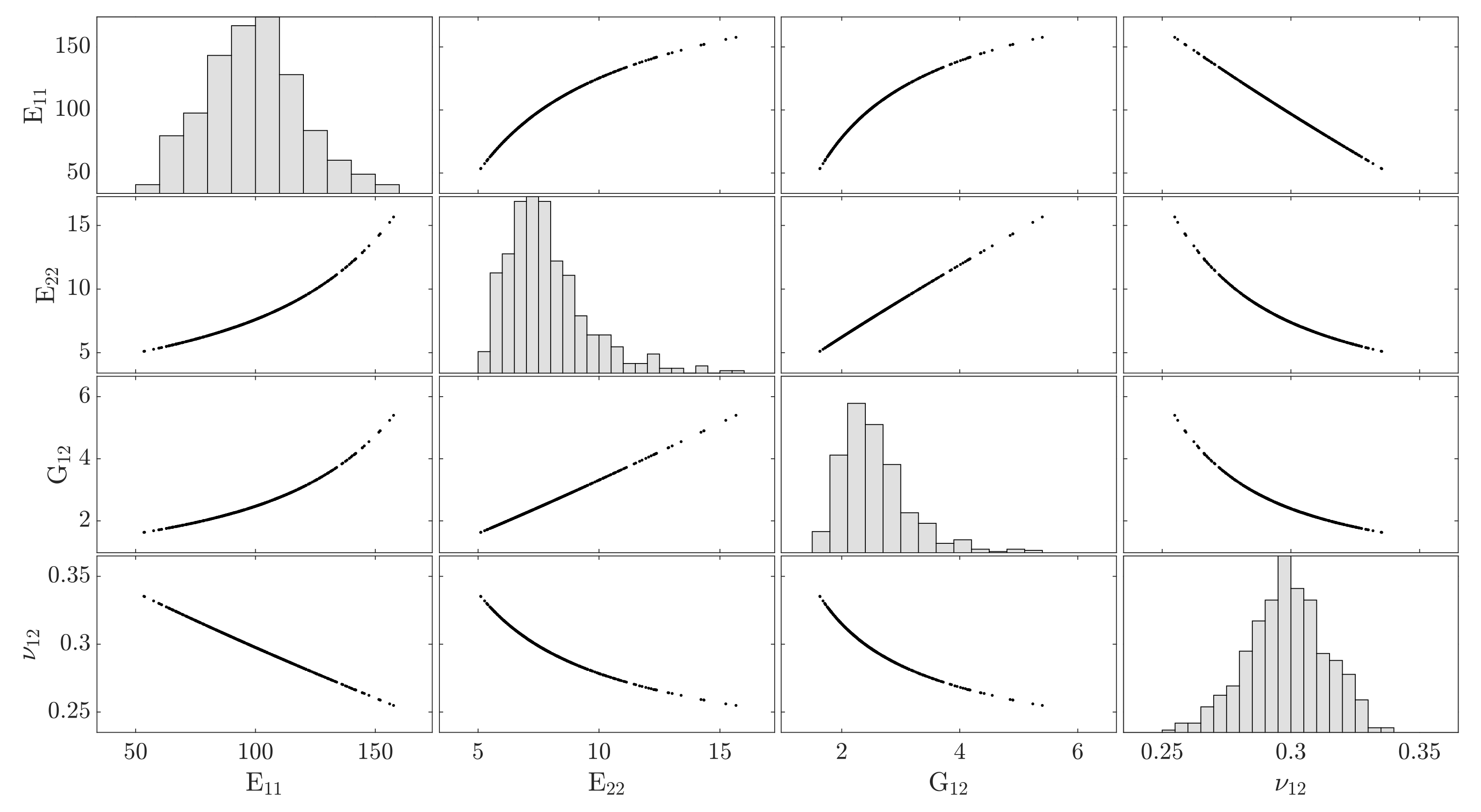
In the first step, a deep learning ANN was employed to construct a predictive model having a data set on the fiber diameter. The set was then split into training and testing sets based on the rule. The major challenge for setting the ANN architecture is the optimal number of hidden layers and neurons to prevent any under- or overestimating. There is no standard and accepted procedure for designing the ANN architecture, i.e., the number and type of neuronal layers and the number of neurons comprising each layer. The initial ANN architecture has to be optimized for eliminating redundant layers and neurons. The number of neurons in the input layer is equal to the number of features of the data, here a column 500 neurons. The output layer has four neurons corresponding to the number of parameters, i.e., and . The number of hidden layers is the most difficult task. The optimal size of the hidden layer is usually set by considering the linear dependency and the size of the input and the output layers. Generally, the number of hidden layers decreases, as the data are linearly separable. Particularly, one needs any hidden layers if data are linear independent. To this end, one may consider the linear dependency of the data by detecting the data correlation, cf. Figure 7.
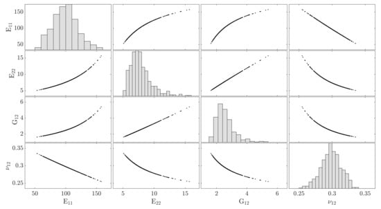
Figure 7.
The qualitative relationships between pairs of parameters. The diagonal plots represent the distribution of parameters. The off-diagonal plots show the linear and nonlinear relationships of the elastic parameters.
The plots show the model relationships between pairs of parameters. This relationship is not linear for all pairs, e.g., and . For that reason, while an ANN model without hidden layers can be used for predication of from randomness in the fiber radius, such a model results in huge error for prediction of other parameters.
One issue is, however, the achieved performance difference from adding additional hidden layers. This has been demonstrated in Figure 8 where the mean-squared error is shown vs. the number of neurons, , for various number of hidden layers, .
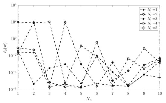
Figure 8.
The performance of ANN vs. number of neurons, , for various number of hidden layers, .
The results show that has minimum error for a single hidden layer with 5 neurons. This setup is used for further results in this paper.
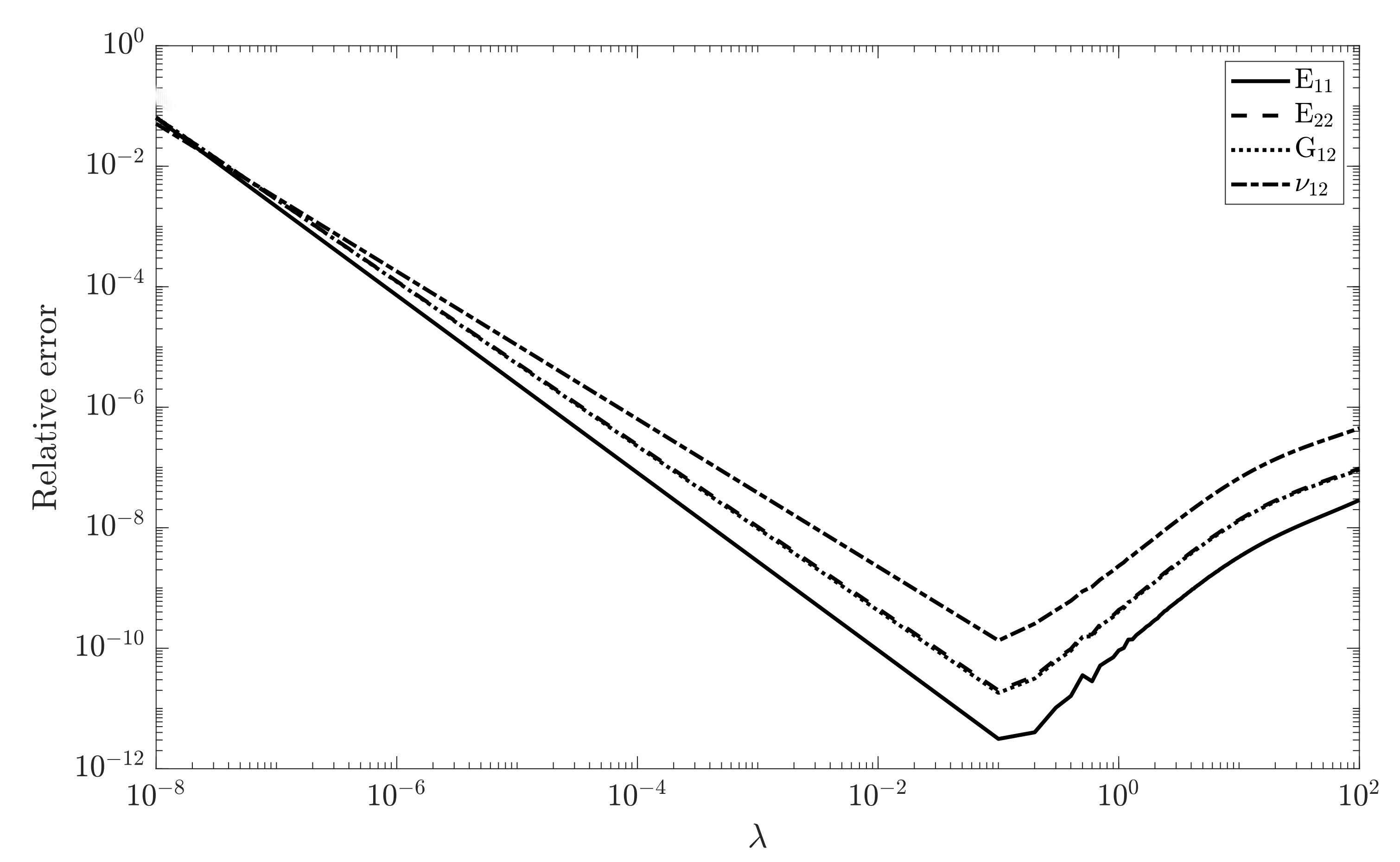
The designed ANN was then used to reconstruct the data from the FE simulations. A set of 500 samples from training distribution , cf. Figure 5, was generated. The training includes of the sample set where are used in testing phase of the model. The training set was chosen randomly. The optimization algorithm requires setting the optimal value for the regulation factor to avoid overestimation of the parameters. This is shown in Figure 9, in which the relative error has been plotted for the training set of all parameters.

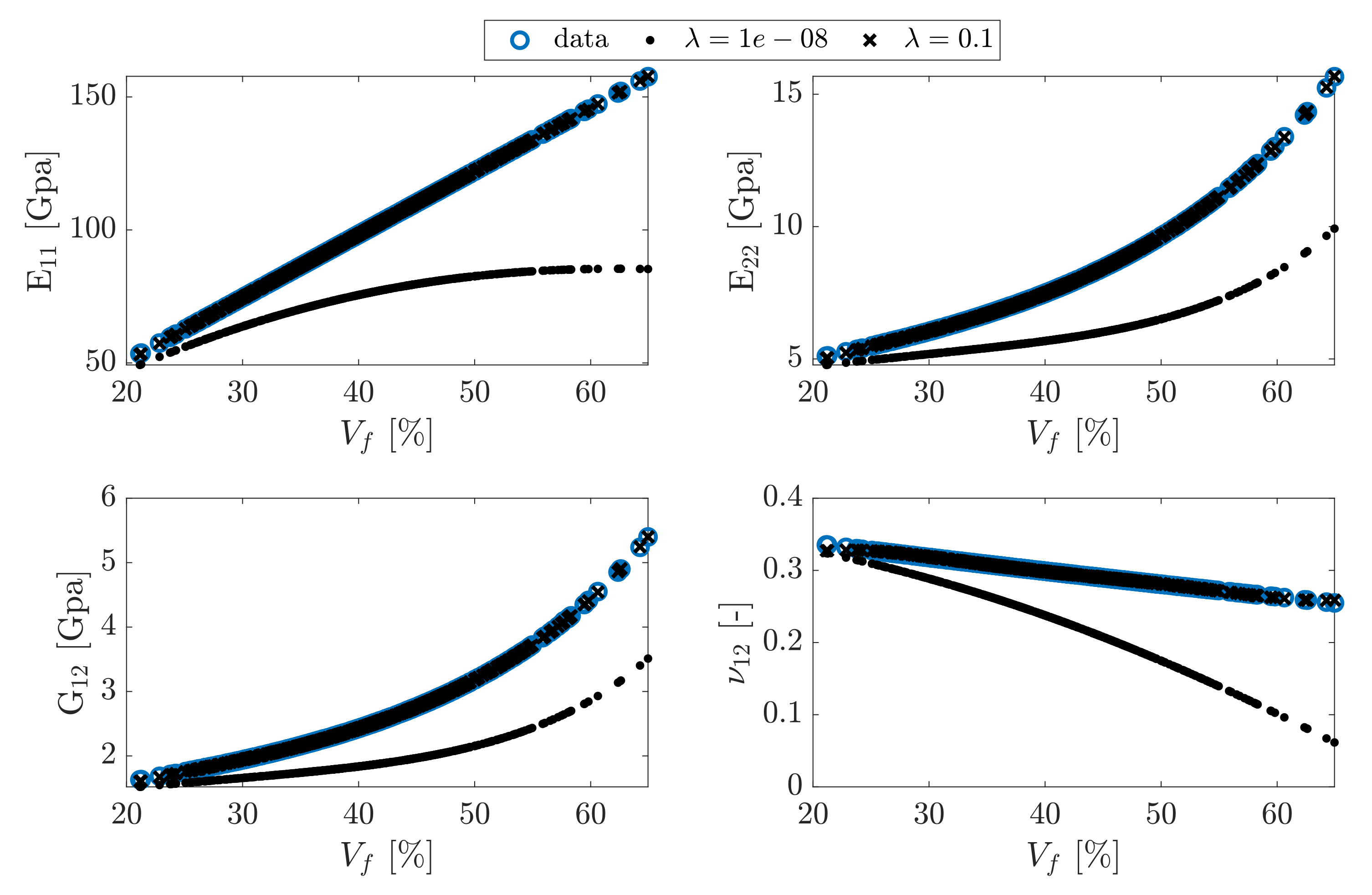
It can be seen that for , the error corresponding to each parameter estimation is minimum. This results in the best fit for all parameters, as shown in Figure 10.

Figure 10.
Data fitting models for and the nonzero value of . The zero value gives obviously huge error in parameter estimation.
The results show a obvious difference between and the nonzero value of , i.e., 0.1.
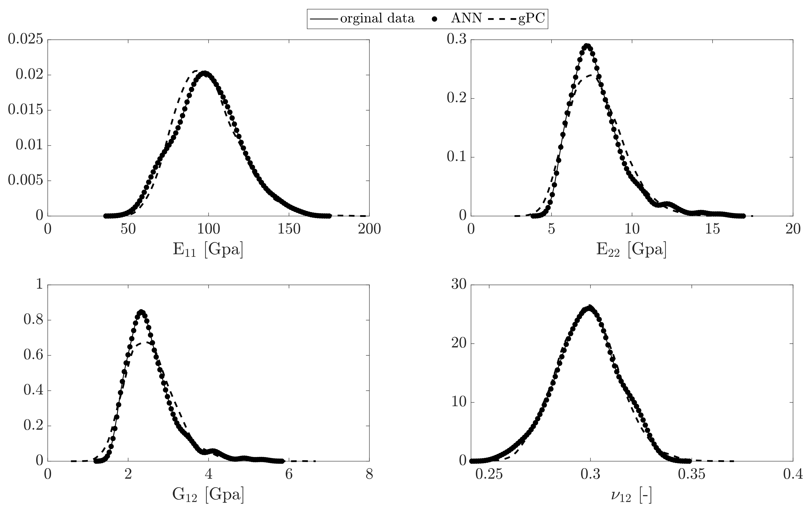
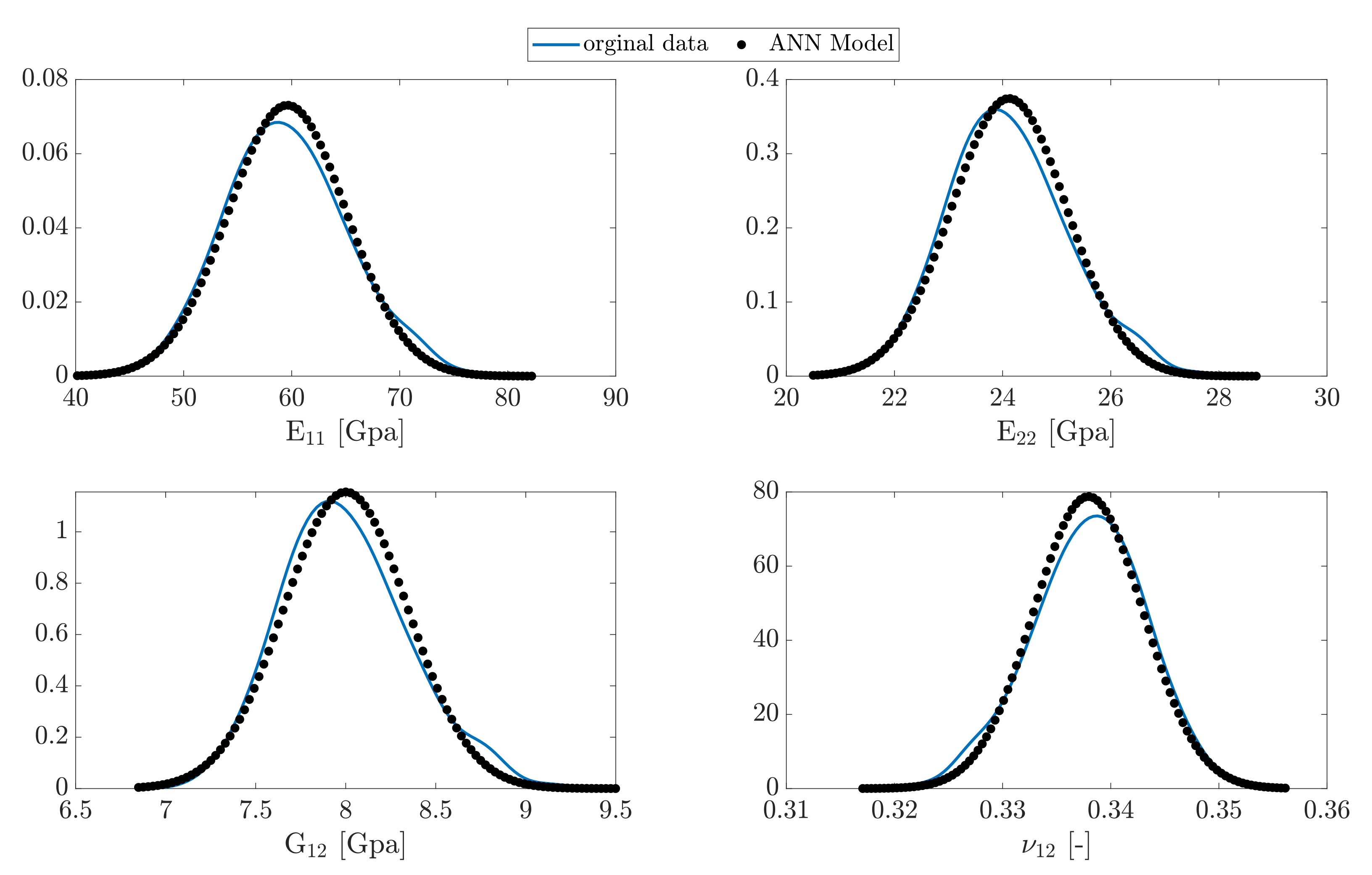
The gradient descent method is used for finding the optimal error function defined as given in Equation (8) employing a maximum of 1000 epochs in each training step. The ANN algorithm is examined for the testing set. The reconstructed PDF of data from the predictive ANN model compared to the original data and the third order Hermite gPC expansions are shown in Figure 11.

Figure 11.
The PDF of the elastic parameters estimated from the ANN model and gPC expansions.
The kernel density method [26] has been used to construct the PDF of the generated data from the ANN model. As shown, the ANN model for each parameter has high accuracy for reconstruction the elastic parameters considering uncertainty in the fiber radius. The variation in the macro-scale material parameters is considerable due to uncertainty in the fiber size (and accordingly the matrix size). Particularly, the wide range of is due to randomness in the diameters of fibers and also randomness in the elasticity in the fiber direction.
To validate the accuracy of the model, a new set of fiber radii are generated from the second PDF, see Figure 5. The non-Gaussian distribution has been reported in [27] for a sample of continuously reinforced polymer (CFRP). The FE code was run for estimation of the elastic parameters. The trained ANN model for the first case was then used to predict the data set for each parameter. The results for the PDFs are demonstrated in Figure 12.
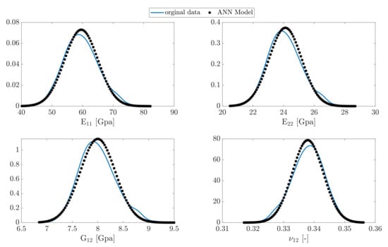
Figure 12.
The predicted PDF of the new data set from the model compared to original data.
As expected, the model has approximately the same accuracy for forecasting the parameters. This is particularly very accurate for estimation of for the new data set owing the fact that the physical relationship between this parameter and the fiber radius is linear.
5. Conclusions
A deep learning ANN model has been developed for prediction of the elastic parameters of the UD fiber lamina using RVE cells from the given probability distribution of the random fiber diameter. Samples of RVE are virtually generated; from there, the probability distribution of the fibers are constructed employing the image processing. Random realizations of the fiber diameter are fed to FE model of the RVE to estimate elastic parameters. The parameters are then utilized to train an ANN having an optimal number of hidden layers and neurons. The predictive model is validated by a set of data from the new distribution of the fiber diameters. The results show that the model has high accuracy for forecasting the elastic parameters.
In contrast to the conventional physical based models, supervised ML models have the ability to be used for future development in material science and engineering. The major challenge is, however, the setting of the optimal architecture of the deep learning ANN, i.e., the number of hidden layers and the affiliated number of neurons. The investigation of relationships between the data can help in this regard. Generally, the number of hidden layers decreases, as the data are linearly separable. For linear independent data, one needs any hidden layer. Once the number of hidden layers has been determined, the number of neurons at each layer is the minimum number corresponding to the optimal layers. This avoids any under- or overestimation of the parameters.
Funding
This research received no external funding.
Institutional Review Board Statement
Not applicable.
Informed Consent Statement
Not applicable.
Conflicts of Interest
The author declares no conflict of interest.
References
- Raju, B.; Hiremath, S.R.; Mahapatra, D.R. A review of micromechanics based models for effective elastic properties of reinforced polymer matrix composites. Compos. Struct. 2018, 204, 607–619. [Google Scholar] [CrossRef]
- Eshelby, J.D.; Peierls, R.E. The determination of the elastic field of an ellipsoidal inclusion, and related problems. Proc. R. Soc. London. Ser. A Math. Phys. Sci. 1957, 241, 376–396. [Google Scholar]
- Hashin, Z. Analysis of Properties of Fiber Composites With Anisotropic Constituents. J. Appl. Mech. 1979, 46, 543–550. [Google Scholar] [CrossRef]
- Peng, X.; Hu, N.; Zheng, H.; Fukunaga, H. Evaluation of mechanical properties of particulate composites with a combined self-consistent and Mori-Tanaka approach. Mech. Mater. 2009, 41, 1288–1297. [Google Scholar] [CrossRef]
- Pathan, M.; Tagarielli, V.; Patsias, S. Numerical predictions of the anisotropic viscoelastic response of unidirectional fiber composites. Compos. Part A Appl. Sci. Manuf. 2017, 93, 18–32. [Google Scholar] [CrossRef]
- Sepahvand, K. Spectral stochastic finite element vibration analysis of fiber-reinforced composites with random fiber orientation. Compos. Struct. 2016, 145, 119–128. [Google Scholar] [CrossRef]
- Karnik, S.; Gaitonde, V.; Rubio, J.C.; Correia, A.E.; Abrão, A.; Davim, J.P. Delamination analysis in high speed drilling of carbon fiber reinforced plastics (CFRP) using artificial neural network model. Mater. Des. 2008, 29, 1768–1776. [Google Scholar] [CrossRef]
- Vakili, M.; Karami, M.; Delfani, S.; Khosrojerdi, S. Experimental investigation and modeling of thermal radiative properties of f-CNTs nanofluid by artificial neural network with Levenberg-Marquardt algorithm. Int. Commun. Heat Mass Transf. 2016, 78, 224–230. [Google Scholar] [CrossRef]
- Stamopoulos, A.; Tserpes, K.; Dentsoras, A. Quality assessment of porous CFRP specimens using X-ray Computed Tomography data and Artificial Neural Networks. Compos. Struct. 2018, 192, 327–335. [Google Scholar] [CrossRef]
- Chen, C.T.; Gu, G. Machine learning for composite materials. MRS Commun. 2019, 9, 556–566. [Google Scholar] [CrossRef] [Green Version]
- Sacco, C.; Baz Radwan, A.; Anderson, A.; Harik, R.; Gregory, E. Machine learning in composites manufacturing: A case study of Automated Fiber Placement inspection. Compos. Struct. 2020, 250, 112514. [Google Scholar] [CrossRef]
- Terada, K.; Miura, T.; Kikuchi, N. Digital image-based modeling applied to the homogenization analysis of composite materials. Comput. Mech. 1997, 20, 331–346. [Google Scholar] [CrossRef]
- Barbero, E.J. Introduction to Composite Materials Design; Tayleor & Francis: Philadelphia, PA, USA, 1998. [Google Scholar]
- Sepahvand, K.; Marburg, S.; Hardtke, H.J. Uncertainty quantification in stochastic systems using polynomial chaos expansion. Int. J. Appl. Mech. 2010, 2, 305–353. [Google Scholar] [CrossRef]
- Yin, X.; Chen, W.; To, A.; McVeigh, C.; Liu, W.K. Statistical volume element method for predicting microstructure-constitutive property relations. Comput. Methods Appl. Mech. Eng. 2008, 197, 3516–3529. [Google Scholar] [CrossRef]
- Roh, Y.; Heo, G.; Whang, S. A Survey on Data Collection for Machine Learning: A Big Data—AI Integration Perspective. IEEE Trans. Knowl. Data Eng. 2019, 1, 1–20. [Google Scholar] [CrossRef] [Green Version]
- Meijaard, J. Applications of the singular value decomposition in dynamics. Comput. Methods Appl. Mech. Eng. 1993, 103, 161–173. [Google Scholar] [CrossRef]
- Tu, J.; Rowley, C.; Luchtenburg, D.; Brunton, S.; Kutz, J. On Dynamic Mode Decomposition: Theory and Applications. J. Comput. Dyn. 2014, 1, 391–421. [Google Scholar] [CrossRef] [Green Version]
- Yuan, Y. Step-sizes for the gradient method. Stud. Adv. Math. 1999, 42, 785–798. [Google Scholar]
- Bishop, C.M. Pattern Recognition and Machine Learning; Springer: Berlin/Heidelberg, Germany, 2006. [Google Scholar]
- Hagan, M.T.; Menhaj, M.B. Training feedforward networks with the Marquardt algorithm. IEEE Trans. Neural Netw. 1994, 5, 989–993. [Google Scholar] [CrossRef]
- Li, M.; Ghosh, S.; Richmond, O.; Weiland, H.; Rouns, T. Three dimensional characterization and modeling of particle reinforced metal matrix composites: Part I: Quantitative description of microstructural morphology. Mater. Sci. Eng. A 1999, 265, 153–173. [Google Scholar] [CrossRef]
- Torquato, S. Statistical Description of Microstructures. Annu. Rev. Mater. Res. 2002, 32, 77–111. [Google Scholar] [CrossRef]
- Baheti, S.; Tunak, M. Characterization of fiber diameter using image analysis. IOP Conf. Ser. Mater. Sci. Eng. 2017, 254, 142002. [Google Scholar] [CrossRef]
- Sepahvand, K.; Marburg, S. On Construction of Uncertain Material Parameter using Generalized Polynomial Chaos Expansion from Experimental Data. Procedia IUTAM 2013, 6, 4–17. [Google Scholar] [CrossRef] [Green Version]
- Silverman, B.W. Density Estimation for Statistics and Data Analysis; Chapman & Hall/CRC: Boca Raton, FL, USA, 1998. [Google Scholar]
- Requena, G.; Fiedler, G.; Seiser, B.; Degischer, P.; Di Michiel, M.; Buslaps, T. 3D-Quantification of the distribution of continuous fibres in unidirectionally reinforced composites. Compos. Part A Appl. Sci. Manuf. 2009, 40, 152–163. [Google Scholar] [CrossRef]


Publisher’s Note: MDPI stays neutral with regard to jurisdictional claims in published maps and institutional affiliations. |
© 2021 by the author. Licensee MDPI, Basel, Switzerland. This article is an open access article distributed under the terms and conditions of the Creative Commons Attribution (CC BY) license (https://creativecommons.org/licenses/by/4.0/).