A Surrogate Model of Heat Transfer Mechanism in a Domestic Gas Oven: A Numerical Simulation Approach for Premixed Flames

Abstract

This paper introduces an innovative analytical model to compute flame velocities and temperatures within a premix burner in a domestic gas oven. This model significantly streamlines the heat transfer simulation process by simplifying the modeling of the thermo-chemical energy release during combustion, effectively reducing complexity and computation time. Accelerated solutions are essential at the initial design stages when comparing the effect of the oven parameter variation on the overall performance. The validation of the proposed analytical model involved experimental assessments of the temperature of the false bottom plate in a natural gas oven. The resulting data were then compared against CFD simulations performed utilizing the proposed model. The results revealed a marginal discrepancy of 4% between the experimental measurements and the outcomes generated by the model. Simulations were executed under differing conditions, encompassing scenarios with and without radiation effects. This exploration identified natural convection as the predominant heat transfer mechanism, with heat radiation contributing only modestly to the heating of the false bottom plate. Among its advantages, the proposed model offers a notable reduction in the numerical complexity of the modeling of the combustion process. Furthermore, its straightforward integration into numerical simulations involving premixed flames underscores its practical utility and versatility in evaluating design performance at the early stages of the design. Highly accurate models can be left for the final oven configuration validation.

1. Introduction

Gas-fueled ovens are extensively used in household food preparation. Within the burner zone, gaseous fuels undergo combustion, supplying thermal energy to the oven system. These ovens incorporate a domestic premix burner, facilitating the chemical oxidation reaction between the fuel and atmospheric air. This reaction results in the liberation of thermal energy within the domestic premix burner structure. Gas ovens exhibit notable advantages compared to their electric counterparts, including quicker heating times and reduced energy expenditure [1]. During the combustion process involving fuel and air, distinct conical flames with a blue tint manifest at the burner ports. The flame configuration corresponds to the Bunsen-type flame [2], which effectively heats the upper surface region known as the false bottom plate (FBP) within the burner zone. The temperature gradient across the FBP is pivotal in furnishing thermal energy to the oven cavity.

Designing ovens involves iteratively testing performance under different parameter settings. The performance is evaluated by running simulations or experiments at various parameter values. The quantification of heat transfer resulting from combustion phenomena can be achieved through experimental measurements or computational simulations. Experimental measurements require carefully placing temperature sensors in specific locations to avoid disrupting the flow dynamics that lead to inaccurate surface temperature predictions [3,4].

On the other hand, numerical simulation entails solving the Navier–Stokes equations for multiple reactive flows, incorporating intricate components such as chemical kinetic mechanisms, reaction rates, species production and destruction rates, and radiation and turbulence models. These simulations demand substantial computational resources and time [5,6]. Thanks to the accessibility provided by current computer power and parallel computing, this type of analysis is now within reach. However, simplified models, due to their advantages in computer time, are preferred for interactive design, optimization design, and control applications, often requiring multiple design performance evaluations. Examples of this include the development of a reduced-order model of an electric oven suitable for design control [7,8], and the use of a reduced-order model of an industrial oven to perform design optimization [9]. This work proposes using a surrogate model to account for the combustion heat transfer effect.

In recent studies, a hybrid approach that combines experimental measurements with numerical simulations is employed to anticipate temperature profiles, flow patterns, and heat transfer mechanisms within thermal devices. Experimental data acquired through measurements serve as input boundary conditions for the numerical simulations, though this amalgamation introduces potential inaccuracies in parameter configurations. Ahanj et al. [10] adopted experimental and numerical methods to study a radiant tube heater. By simulating the combustion process within the burner, they prognosticated the impact of various variables involved in the phenomenon and the resulting temperature distribution along the radiant tube. Similarly, Cadavid et al. [11] conducted combustion simulations to forecast heat transfer and fluid flow within an auto-regenerative crucible furnace. They harnessed two distinct combustion models: the PDF mixture fraction and Finite Rate/Eddy Dissipation models. Nevertheless, the computational simulation of combustion processes for heat transfer estimation introduces a notable escalation in computational time requirements for predicting furnace working temperatures.

To address this complexity, various alternative approaches have been suggested. Karzar Jeddi and colleagues [12] employed the finite element method to reproduce the heat convection from a gas stove burner hitting the bottom of a cooking pot. Similarly, Wong et al. [13] utilized computational tools to emulate the intricate interactions across all compartments within an oven specifically designed for baking dough and bread. Additionally, Mistry et al. [14] conducted a comprehensive three-dimensional numerical simulation of a domestic gas oven. Their approach focused solely on simulating the oven cavity, utilizing experimental measurements to spatially delineate the temperature distribution on the false bottom plate (FBP). Notably, the simulation of temperatures and fluid velocities arising from the combustion process was circumvented, instead drawing from prior experimental data and incorporating these values as boundary conditions within the model. However, this reliance on experimental data constitutes a noteworthy drawback of the derived numerical results, given the challenges in acquiring precise experimental measurements and the potential for introducing errors.

A primary constraint of this methodology arises when alterations occur in the operational parameters of the heat source, necessitating fresh rounds of experimental measurements to establish a revised set of boundary conditions. This study introduces an analytical framework grounded in Bunsen-type flame theory and impinging-flame jet principles to address this limitation. This framework aims to compute the velocities and temperatures associated with the heat source within the burner zone of a residential gas oven. The analytical model proposed in this work is benchmarked against the empirical investigation conducted by Hou and Ko [15], as well as the numerical combustion simulations by Agrawal et al. [16]. Furthermore, experimental temperature measurements performed on a natural gas oven’s false bottom plate (FBP) are juxtaposed with the outcomes derived from the analytical model. A notable attribute of the proposed analytical model is its capability to surmount the aforementioned limitations. When the operational condition changes, this model recalibrates the boundary conditions analytically, circumventing the need for additional experimental measurements.

2. Materials and Methods

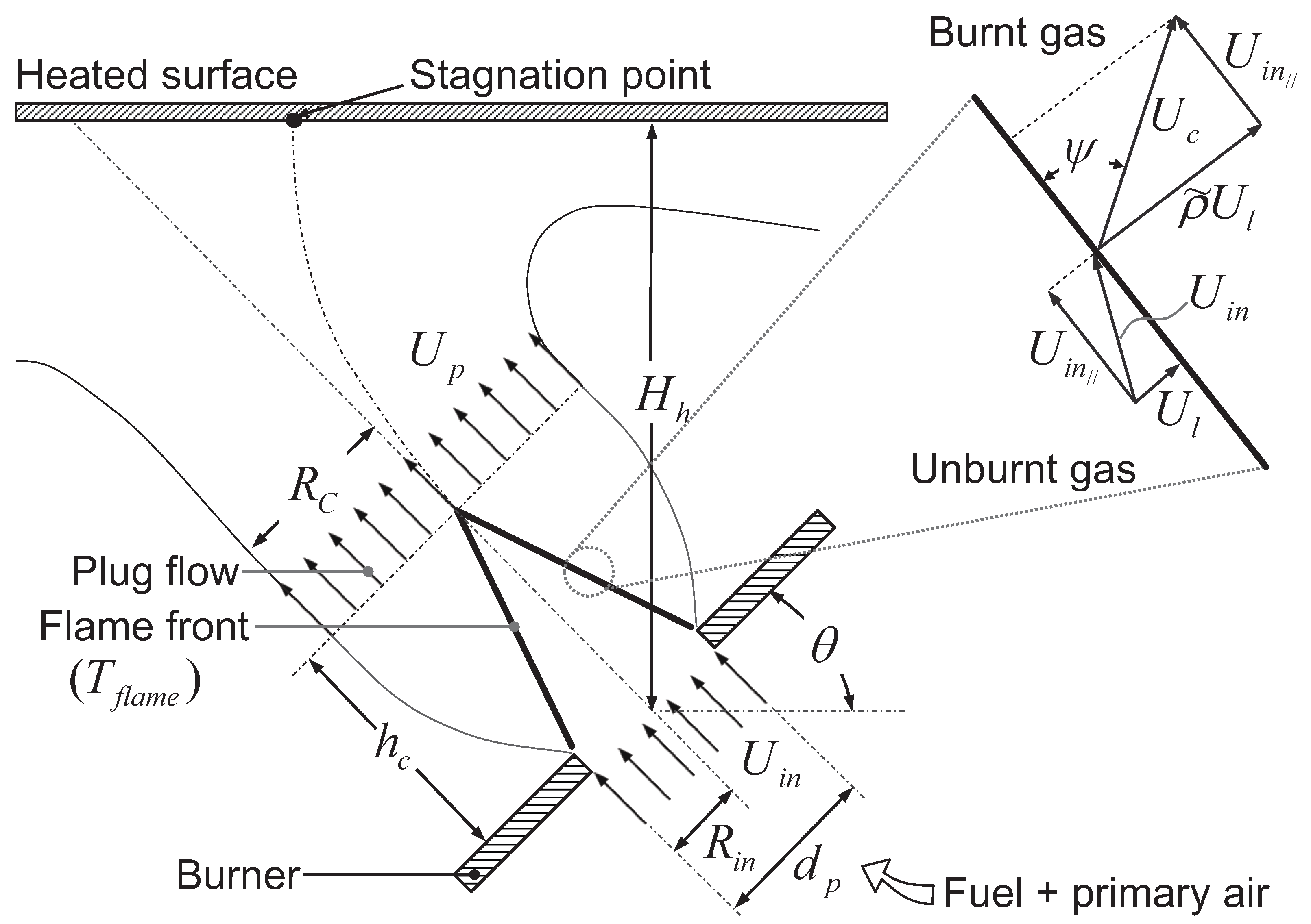
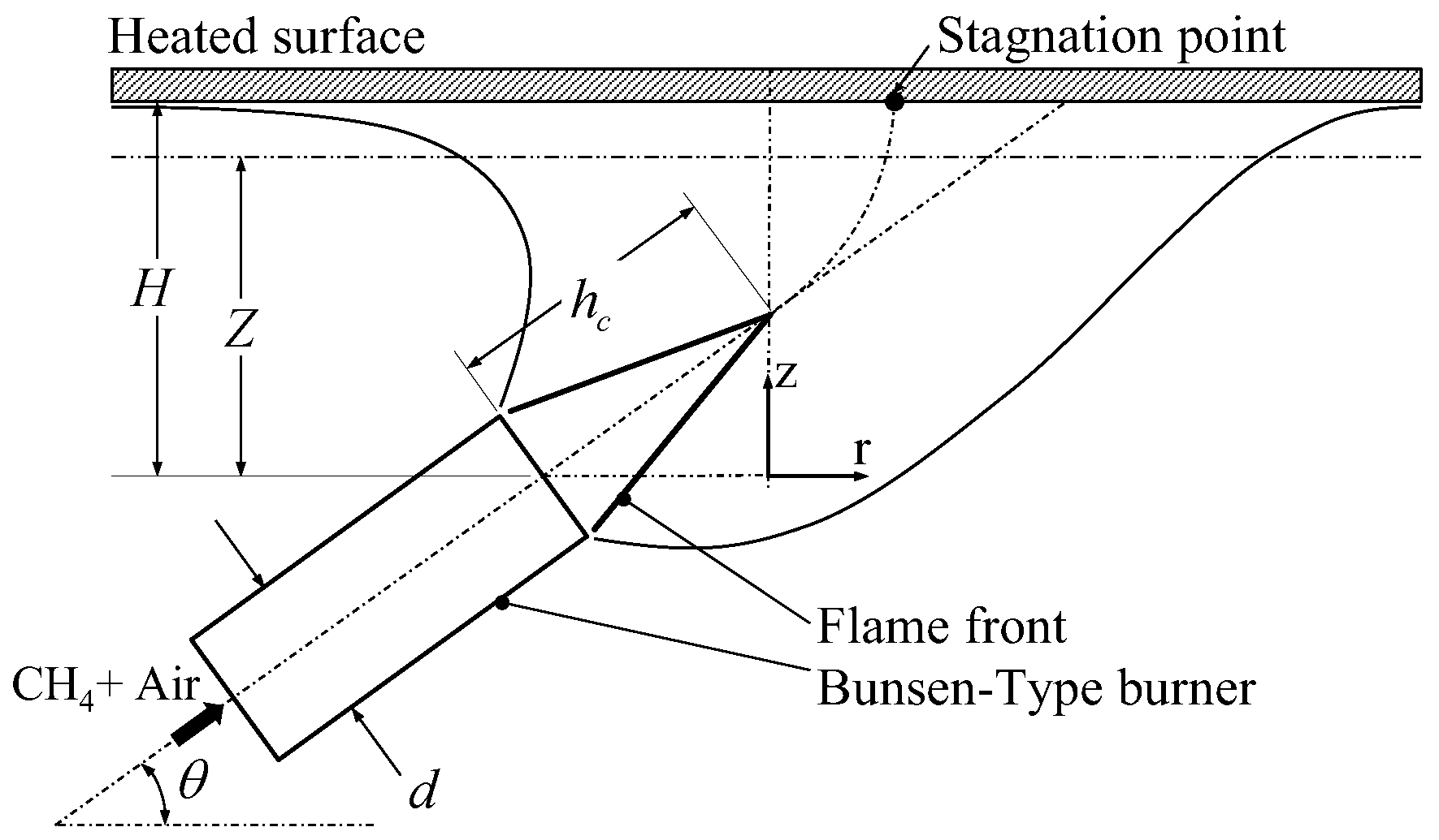
2.1. Analytical Modeling of Heat Transfer Mechanisms in Premix Gas Oven Burners

The combustion of the fuel and air mixture initiates an exothermic chemical reaction along the flame front. Simulating this process is computationally demanding. The heat transfer from impinging premixed flame jets to a surface is multifaceted, encompassing diverse heat transfer mechanisms like conduction, convection, radiation, and thermochemical heat release [17,18]. To streamline the numerical simulation of thermal energy transfer from a premixed burner in a gas oven, an analytical model is proposed, integrating the subsequent components: (i) A Bunsen-type flame model to ascertain the resultant velocity vector arising from the combustion products at the flame forefront, denoted as $U_C$. (ii) The impinging premixed flame jets theory to calculate the various mechanisms governing heat transfer from the flame to the heated surface. (iii) Chemical equilibrium principles to compute the heat generated during the chemical reaction between methane and air. The outcomes of this model, encompassing temperature and velocities, serve as foundational boundary conditions on a cone-shaped surface replicating the flame forefront within the computational domain. A schematic representation of this particular flame configuration is depicted in Figure 1.

The adiabatic flame temperature, denoted as $T_{\mathrm{flame}}$, and the volume of combustion products were computed based on the equivalence ratio using the GasEq software, Ver.0.79, by Chris Morley [19]. These combustion products were streamlined to eleven species: CO₂, CO, H₂, H, H₂O, OH, O₂, O, NO, N₂, and N. The adiabatic flame temperature ($T_{\mathrm{flame}}$) indicates the heat generated within the burner zone by the flame. The inflow velocity at the main burner ports, represented as $U_{in}$, was derived from the combined rates of the fuel ejecting from the injector and the primary air being drawn into the burner. The methane burning velocity ($U_{lo}$) was calculated utilizing the equivalence ratio ($\varphi$) and the correlation established by El-Sherif [20]:

$$U_{lo}=0.37{\varphi }^{-0.35}exp\left[-5{\left(\varphi -1.1\right)}^2\right],$$

(1)

the burning velocity $U_{lo}$ has to be corrected for pressures lower than atmospheric pressure and at a temperature of 300 K,

$$U_l=U_{lo}{\left(\frac{P_u}{P_0}\right)}^{-0.14}.$$

(2)

The term $U_l$ denotes the corrected burned velocity, as illustrated in Figure 1. As combustion products traverse the flame front, they undergo a distinct acceleration due to the density disparity between the unburned and burned gases. This variation in density propels an uptick in the gas velocity. Let us represent the density ratio of the unburned gases to the burned gases as $\tilde{\rho }$ [21]. For a Bunsen-type flame in 2D, the velocity of the burnt gases at the flame front, labeled as $U_c$, was established by Remie et al. [22] as follows:

$$U_c^2=U_{in}^2+U_l^2\left({\tilde{\rho }}^2-1\right),$$

(3)

and, considered uniform over the whole surface of the flame front, leaving at angle $\psi$,

$$cos\psi =\frac{U_{{in}_{//}}}{U_c},\mathrm{with}{U}_{{in}_{//}}^2={U_l}^2+{U_{in}}^2,$$

(4)

where the subscript $U_{i{n}_{//}}$ stands for the component parallel to the flame direction (see Figure 1). The flame shape can be described by its main geometric parameters, which are the diameter of the burner output main port, $d_p$; the heating height, $H_h$; the flame angle, $\theta$; and the cone height, $h_c$. These parameters can be calculated using the equation given by Kleijn [23],

$$\frac{h_c}{d_p}=\frac{U_{in}}{2U_l}.$$

(5)

Other heat transfer mechanisms in premixed flames of a gas oven are thermo-chemical heat release and the heat transfer of luminous and non-luminous radiation. The influence of thermo-chemical heat release is minimal for methane/air mixtures because N₂ functions as a heat sink [24]. For gaseous fuels like methane, the impact of luminous radiation is diminished due to the absence of soot particles in the combustion products. Additionally, non-luminous radiation is negligible in the presence of methane/air because combustion products like CO₂ and H₂O exhibit low emissivity [25]. Furthermore, the flame front’s shape undergoes alterations due to buoyancy effects, which can be quantified using the Froude number [26].

To focus on the dominant mechanism, this study solely considers convective heat transfer. Other heat transfer contributions from methane/air combustion products are neglected, as explained previously. Additionally, no buoyancy effects from the burnt gases on the flame front were considered. In summary, in this analytical framework, the heat released in the chemical reaction was depicted by the temperature of the adiabatic flame, which was determined through chemical equilibrium. Equations (3) and (4) are employed to deduce the velocity of the burnt gases and their respective angles. Subsequently, the CFD simulation receives fluid velocity and temperature across the conical surface as boundary conditions. The CFD domain captures the conical geometry of the flame front, characterized by the primary burner output’s diameter and the cone’s height as denoted by Equation (5). Notably, secondary air, essential for the completion of combustion, is not accounted for in this model.

2.2. Numerical Model (CFD)

The air inside the oven was modeled as turbulent and non-reactive fluid. The equations for conservation of mass, momentum, and energy are given by:

$$\begin{array}{cc}\hfill \frac{\partial \rho U_j}{\partial x_j}=& 0,\hfill \\ \hfill \frac{\partial \rho U_j{U}_i}{\partial x_j}=& -\frac{\partial P}{\partial x_i}+\frac{\partial }{\partial x_j}\left[\mu \left(\frac{\partial U_i}{\partial x_j}+\frac{\partial U_j}{\partial x_i}\right)\right.\hfill \end{array}$$

(6)

$$\begin{array}{cc}\hfill & \left.-\frac{2}{3}\mu {\delta }_{ij}\frac{\partial U_k}{\partial x_k}-\rho \overline{u_i^{\prime }{u}_j^{\prime }}\right]+\left(\rho -{\rho }_{ref}\right)g_i,\hfill \end{array}$$

(7)

$$\begin{array}{cc}\hfill C_p\frac{\partial U_{j}T}{\partial x_j}=& \frac{\partial }{\partial x_j}\left(\frac{\mu C_p}{Pr}\frac{\partial T}{\partial x_j}\right)+\frac{\partial }{\partial x_j}\left(-\rho C_p\overline{u_j^{{ }^{\prime }}{T}^{\prime }}\right).\hfill \end{array}$$

(8)

Due to the large temperature differences present in the problem, the buoyancy term $(\rho -{\rho }_{ref})g_i$ in (7) was solved with the non-Boussinesq approach [27]. The reference density used was ${\rho }_{ref}$= $1.184$ Kg/$m^2$, which corresponded to $298.5$ K. The turbulent heat flux vector, $-\rho C_p\overline{u_j^{\prime }{T}^{\prime }}$, in the energy equation is given by:

$$\begin{array}{c}\hfill -\rho C_p\overline{u_j^{\prime }{T}^{\prime }}={\lambda }_t\frac{\partial T}{\partial Z},{\lambda }_t=\frac{{\mu }_t{C}_p}{P{r}_t}\mathrm{with}P{r}_t=0.9.\end{array}$$

(9)

The Rayleigh number $Ra=g\beta (T_{wall}-T_{\infty })L^3/\nu \alpha$ at the cavity was $1.649\times {10}^6$, indicating turbulent flow within the oven cavity [28]. To address this turbulence and improve the accuracy of heat transfer predictions near the walls, the Shear Stress Transport (SST) two-equation turbulence model was employed [29]. This choice yielded results better aligned with experimental data than other turbulence models [30,31].

The dynamic viscosity $\mu \left(T\right)$ and the thermal conductivity $\lambda \left(T\right)$ of air, modeled as an ideal gas, were computed from the Sutherland equations [32]. The specific heat capacity $C_p\left(T\right)$ was obtained using the tabulated experimental data from [33]. A fourth-order polynomial regression was used to fit the data. The resulting equation, with an R-squared of $0.9986$, is:

$$\begin{array}{c}\hfill C_p\left(T\right)=968.94+5.88\times {10}^{-2}T+2.4851\times {10}^{-4}{T}^2\\ \hfill -1.601\times {10}^{-7}{T}^3+2.872\times {10}^{-11}{T}^4.\end{array}$$

(10)

The core equations governing mass conservation, momentum, energy, and turbulence were numerically addressed utilizing the finite volume method in ANSYS CFX. An upwind scheme was adopted for the convective components of the momentum and energy equations. The SIMPLE algorithm facilitated the coupling of pressure and velocity. A $y^{+}\approx 1$ value was consistently upheld on the wall to ensure precision within the SST model. Thermal radiation emanating from the burner zone’s surfaces was ascertained via the Monte Carlo method, incorporating the surface-to-surface (S2S) model. Convergence for the simulation was determined based on both the maximum and average temperatures within the FBP. To ensure a converged and accurate solution, the residuals for continuity, momentum, and energy equations were set to a strict convergence criterion of ${10}^{-5}$. Additionally, a double-precision solver was utilized to minimize errors introduced by rounding during calculations.

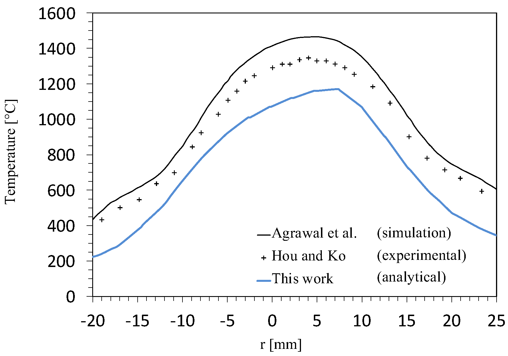
3. Validation of the Analytical Model

The model described in Section 2.1, which estimates the heat transfer rate during the combustion process within the gas oven, underwent validation through two distinct means: First, it was benchmarked against the experimental findings of impinging premixed flame jets by Hou and Ko [15]. Secondly, it was juxtaposed with a numerical simulation centered on the combustion dynamics for a similar flame, as studied by Agrawal et al. [16]. Notably, all these studies operated under identical burner assembly conditions. A schematic representation of the Bunsen-type burner, utilized to validate the analytical model, can be viewed in Figure 2.

The air temperature distribution along the middle plane on the stagnation point (Z-r plane) is shown in Figure 3. A comparison reveals a relative discrepancy of $17.4\%$ between the experimental findings of Hou and Ko [15] and the proposed analytical model. In contrast, there is a $9.9\%$ difference between the results of Hou and Ko [15] and those of Agrawal et al. [16]. Notably, while the analytical model appears to underestimate the temperature, the CFD simulation skews towards an overestimation.

4. Numerical Setup

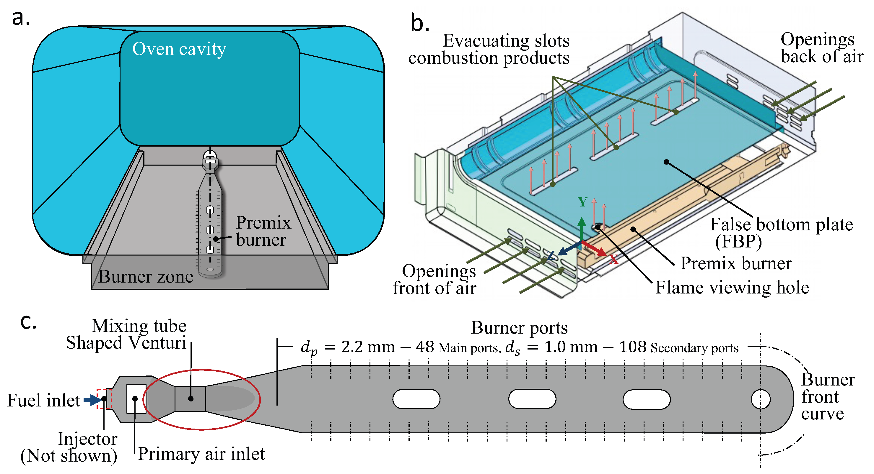
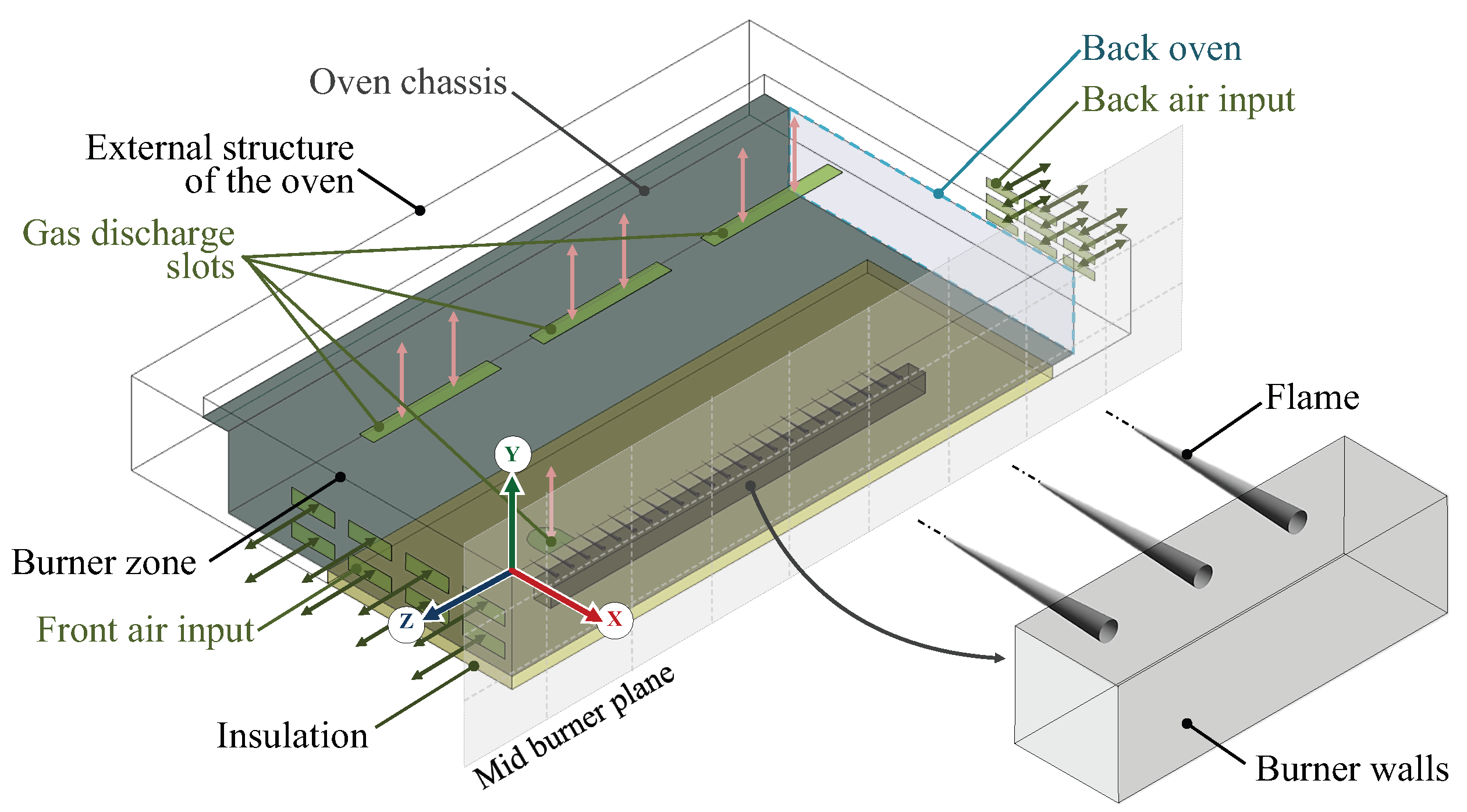
4.1. Burner Zone Description

In Figure 4a, a schematic depiction of the burner zone within the domestic gas oven utilized in this study is presented. Situated at the bottom of the oven cavity, the burner zone features a centrally positioned premix burner along the x-axis, positioned below the FBP at a distance of $H_h=36$ mm along the y-axis. The premix burner is responsible for heating the oven. As illustrated in Figure 4b, the combustion products generated by the burner heat the surface of the FBP. Additionally, six gas evacuation slots on the FBP (three on each side) facilitate the passage of combustion products from the burner zone into the oven cavity.

The burner zone incorporates openings on both the front and rear sides of the oven chassis, facilitating the entry of air required for the combustion process, as depicted in Figure 4c. Natural gas is introduced into the premix burner via an injector that draws in primary air from the surrounding environment. Within a venturi-shaped tube, the fuel and air blend to achieve homogeneity. Upon exiting the burner ports, the mixture combines with secondary air to finalize the combustion process. Electronic ignition is employed for combustion initiation. In this analysis, the focus is placed solely on the primary ports for determining speed and temperature within the burner. In contrast, the secondary ports, primarily utilized for flame stabilization, are excluded from the analysis.

The injector released a natural gas flow of 5 L/min, under a supply pressure of 20 mbar and at a temperature of $298.5$ K, conforming to typical domestic usage conditions. Since methane is the main component of natural gas, pure methane properties were considered to compute the power output of $1982$ kW based on methane’s lower heating value (LHV). For oxidation, atmospheric air comprising $21\%$ O₂ and $79\%$ N₂ was employed. The flow emerging from the premix burner ports was computed using an equivalence ratio of $\varphi =1.663$, under an atmospheric pressure of $0.85$ atm and a temperature of $298.5$ K. The equivalence ratio was determined experimentally based on the methane fraction within the pre-mixture [34].

4.2. Boundary Conditions

Figure 5 illustrates the boundary conditions employed in the simulation, which include:

• Front air input, back input, and gas discharge slots: These are treated as opening boundaries with a relative pressure of 0 Pa and a temperature of 300 K.
• Flame: Modeled as a cone with the adiabatic flame temperature, $T_{flame}$, and the combustion products velocity, $U_c$, in cylindrical coordinates relative to its axis of rotation. These values remain constant across the entire surface of the cone, as determined by the analytical model outlined in Section 2.
• Burner walls: Subjected to a non-slip condition on the burner surface and treated as adiabatic surfaces.
• Mid burner plane: This is a symmetry plane. Given the shape and location of the thermal energy source within the oven, only the left half of the domain was simulated.
• Oven chassis and back oven: Defined as fluid-solid and fluid-fluid interfaces, respectively. Non-slip conditions apply to the interface surfaces, with the conservation of heat flux ensured at these boundaries.

Surfaces and interfaces not explicitly addressed previously were assigned a turbulence intensity of 5%, along with non-slip and adiabatic conditions. Regarding heat radiation simulation, the local ambient temperature was applied to the inputs, outputs, and open boundaries. The emissivity value for the metallic oven surfaces was determined from surface finish tables and corresponded to 0.9 [35].

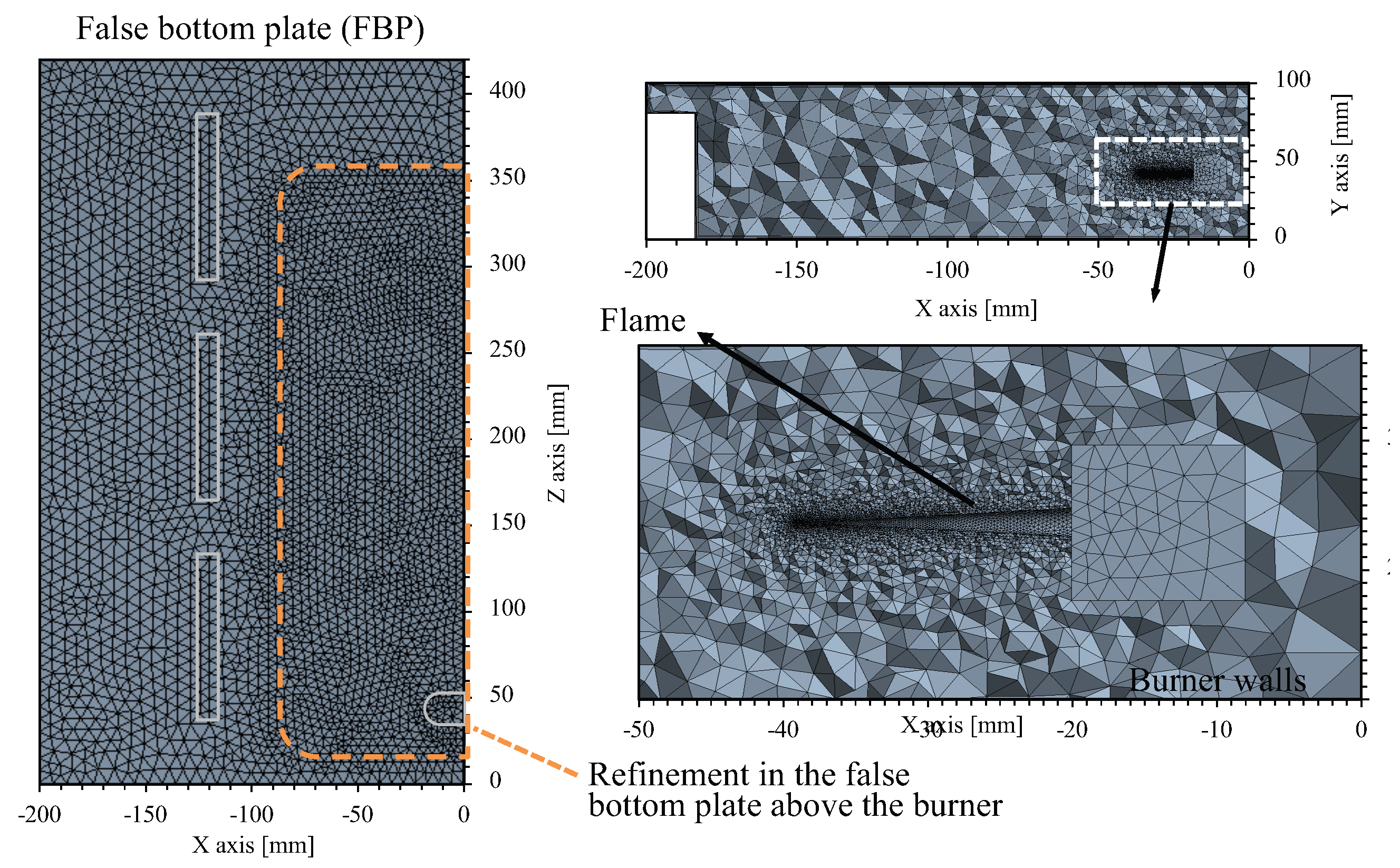
4.3. Mesh and Grid Independence Study

Mesh generation posed challenges due to significant variations in geometric features’ sizes. Unstructured meshes were generated for the computational domains of the burner zone. Specifically, refining the FBP surface above the burner was imperative to enhance numerical accuracy in temperature results obtained from the simulation. These mesh adjustments are illustrated in Figure 6.

A grid independence study was conducted to assess the accuracy of numerical simulation results, as presented in

Table 1. Mesh independence study. Comparing average and maximum temperatures on the false bottom plate using different mesh densities.

Mesh	Elements	Nodes Plate	${\mathit{y}}^{+}$	${\mathit{T}}_{\mathit{a}\mathit{v}\mathit{e}}$ (K)	${\mathit{T}}_{\mathit{m}\mathit{a}\mathit{x}}$ (K)	time (h:m:s)
1	3,598,576	757,098	0.492	589.063	677.349	07:10:36
2	4,111,743	763,278	1.09	595.62	695.89	12:20:11
3	5,437,027	1,066,570	0.494	598.305	697.5	18:51:20

. The analysis reveal marginal differences of $0.45\%$ for average temperature ($T_{ave}$) and $0.23\%$ for maximum temperature ($T_{max}$) between mesh 2 and mesh 3. Notably, mesh 2 demanded 6 h less computing time. Consequently, a mesh comprising 4,111,743 elements (Mesh 2) was deemed adequate for achieving a reliable solution with minimal computational expense.

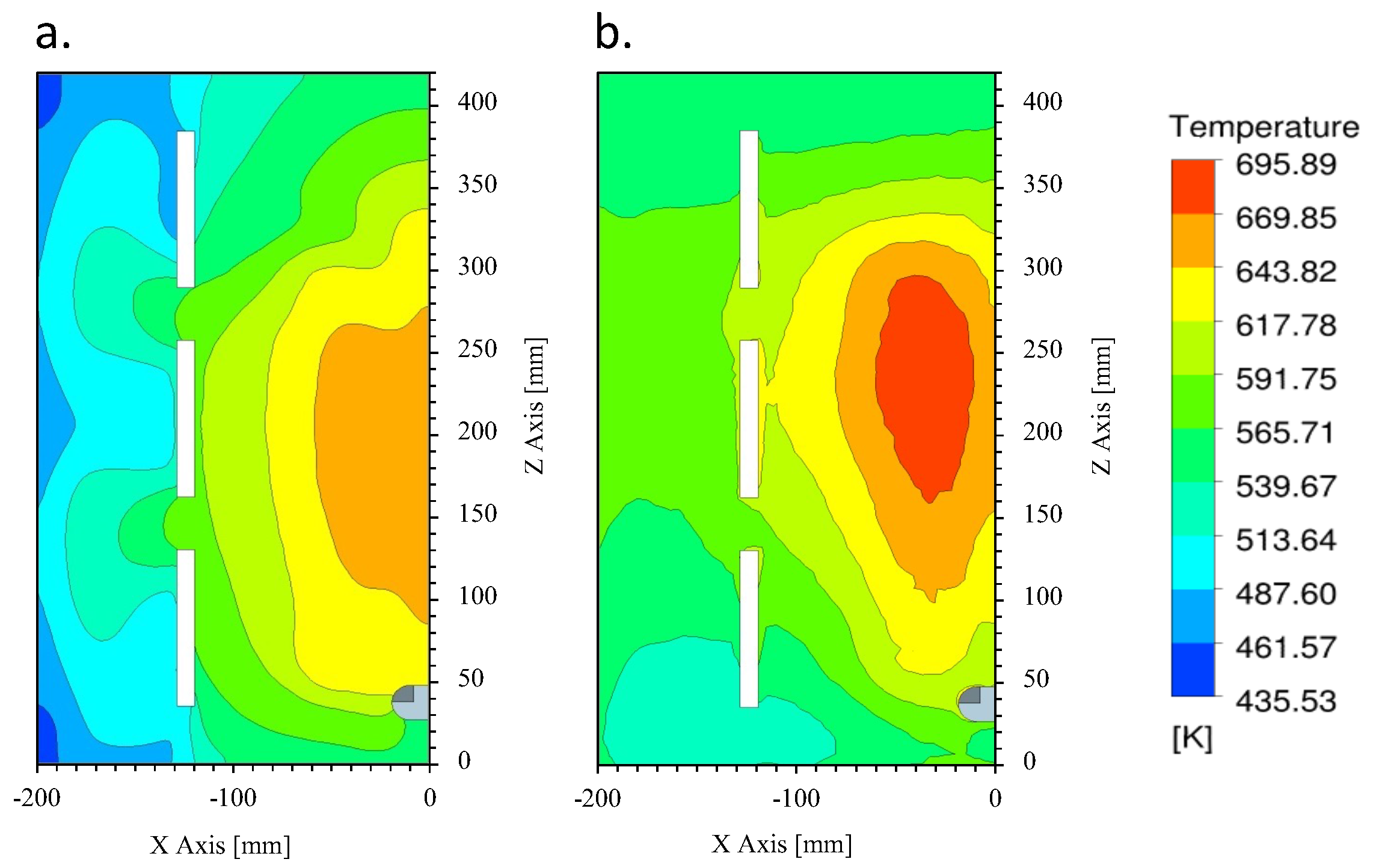
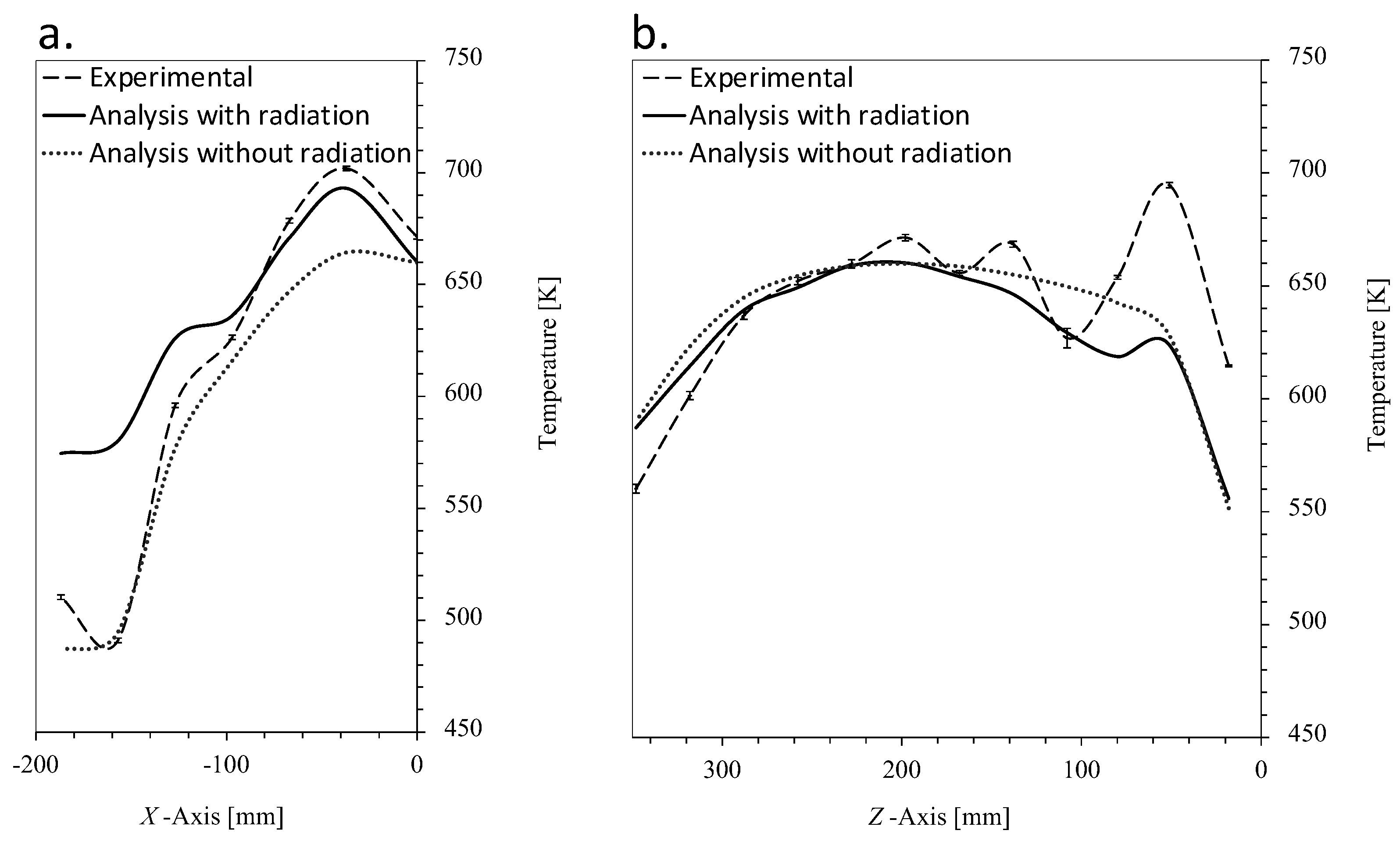
5. Results and Discussion

Given that heat transfer to the oven cavity occurs via the false bottom plate (FBP), the primary objective of the simulations was to compute the temperature distribution across the FBP. Two distinct simulations evaluated the heat transfer mechanisms from the premix burner to the oven cavity. The initial simulation solely accounted for natural convection while disregarding radiative heat transfer. In contrast, the second simulation incorporated natural convection and radiative heat transfer.

The burner zone has several circulating air inlets that interact with the hot air coming from the flame surface proposed by the present model, as shown in Figure 7.

Figure 8 illustrates the surface temperature contours of the FBP under two conditions: with and without radiation. The hot gases from the premix burner heat all surfaces within the burner zone. Notably, the maximum temperature on the FBP was located above the premix burner. With the inclusion of radiation, this region retained its status as the area with the highest temperature. Moreover, the temperatures across the entire FBP escalated due to radiant exchange among the hot surfaces within the burner zone.

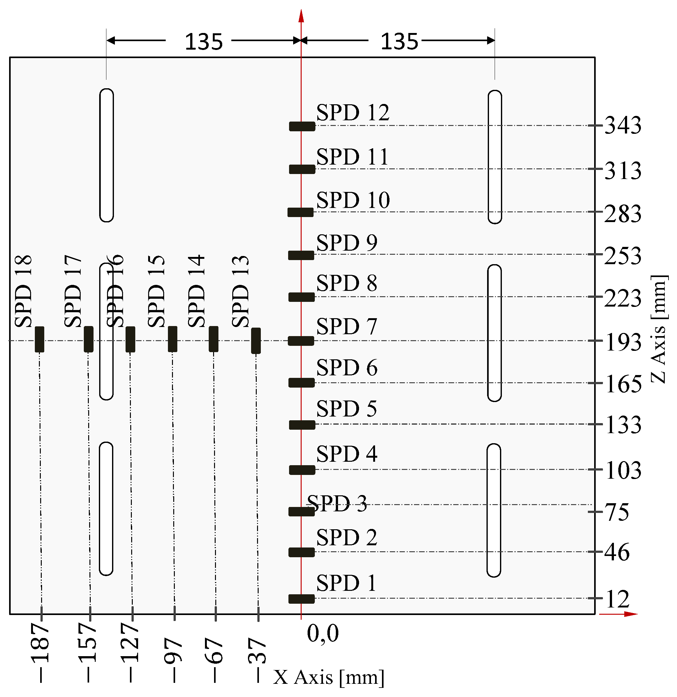
Experimental Validation

To validate this simulation, the temperature on the FBP was measured using 18 type-K thermocouples encased in stainless steel shells with a diameter of 6 mm. Twelve thermocouples were positioned along the centerline of the FBP (z-axis), while the remaining six were located on the left half of the FBP (x-axis). All thermocouples were securely attached to the FBP surface with a metallic structure, strategically placed on the cavity side to avoid interference with the flow of combustion products within the burner zone (refer to Figure 9). Data collection was facilitated by a multilogger thermometer gauge calibrated with an accuracy of $\pm 0.01$ °C, as per [36]. An environment-controlled system maintained a constant ambient temperature of $25$ °C.

The temperatures recorded on the FBP for each analysis are depicted in Figure 10. Error bars accompanying the experimental measurements were determined from three measurements conducted throughout the day (morning, afternoon, and night) during the gas oven’s operational cycle. These error bars were computed using $\sigma /\sqrt{n}$, where $\sigma$ represents the standard deviation of the sample and n indicates the number of experiment repetitions. The data were organized into vectors, and the relative error between experimental and simulated data was calculated as ${\Vert A-B\Vert }^2/{\Vert A\Vert }^2$, where A represents simulation data and B represents experimental data. The relative error between experimental data and the simulation without radiation amounted to $4.47\%$, while the relative error between experimental data and the simulation with radiation was $5.85\%$.

As depicted in Figure 10, the temperature profile obtained from the simulation incorporating radiation closely matches the experimental data within the x-axis range from $-100$ mm to 0 mm. This correspondence can be attributed to the burner and flame surfaces positioned at $X=-40$ mm below the FBP, effectively heating the FBP through radiation. Consequently, the emissivity of these surfaces significantly contributes to the elevated temperatures in this region as the combustion products play a negligible role in radiation-based heat exchange. Conversely, for values falling within the range of $-187$ mm to $-100$ mm, the temperatures calculated by the simulation without radiation exhibit a closer alignment with the experimental data. This discrepancy arises because the cone-shaped surface of our analytical model, representing the flame, does not partake in heat exchange within this region.

In terms of temperatures along the z-axis, simulations with and without radiation displayed a discrepancy of $1.62\%$. A noticeable pattern emerges in the temperature curve: an initial rise in temperature, followed by a period of temperature stabilization, and ultimately a decline in temperature as the distance along the z-axis increases. During the initial phase of sustainment (spanning Z values from $0.0$ mm to 230 mm), the experimental temperature curve exhibits oscillatory fluctuations. These fluctuations are attributed to a hole on the front side of the FBP, which exposes the flame. Some high-temperature combustion products exit the burner zone through this hole, contributing to the observed temperature oscillations. This behavior is less pronounced in the temperature curve without radiation, while the curve with radiation displays it to a lesser extent. The observed discrepancies could be attributed to simplifications in the burner geometry, such as the absence of curvature at the tip in the burner model and the lack of secondary ports.

6. Conclusions

An analytical model was developed to estimate the velocities and temperatures of a premix burner flame in a domestic gas oven, circumventing the need for computationally expensive simulations of the combustion process within the burner.

This model establishes boundary conditions over the ports of a premix burner without directly addressing thermochemical heat release. Through numerical validation against existing literature data, we found the analytical model to be accurate, with a maximum relative error of $17.4\%$. This demonstrates favorable agreement with the reported values.

Experimental temperature distribution measurements were conducted across the false bottom plate (FBP) within the domestic gas oven. The thermocouples were positioned on the side of the oven cavity to prevent interference with the flow of combustion products. A comparison of temperature distribution data, with and without accounting for heat radiation modeling, revealed a discrepancy of $4.5\%$. Based on this finding, we conclude that natural convection is the dominant heat transfer mechanism in the burner zone.

The proposed analytical model significantly reduces computational costs by minimizing the number of equations required to solve the combustion process. Moreover, this analytical model can be extended to various sophisticated devices, enabling the prediction of thermochemical heat transfer from a premix burner flame to a surface. This extension helps streamline the complexity of numerical simulations in diverse applications.

The proposed model stands out for its simplicity, significantly reducing the complexity of simulating the combustion process. This makes it ideal for early-stage design evaluations, allowing for quick performance assessments. More computationally expensive high-fidelity models can then be reserved for final oven validation.

References

1. Ryu, J.; Kwon, J.; Kim, R.; Kim, M.; Kim, Y.; Jeon, C.; Song, J. Surface ignition behaviors of methane–air mixture in a gas oven burner. Appl. Therm. Eng. 2014, 65, 262–272. [Google Scholar] [CrossRef]
2. Gotoda, H.; Maeda, K.; Ueda, T.; Cheng, R.K. Periodic motion of a Bunsen flame tip with burner rotation. Combust. Flame 2003, 134, 67–79. [Google Scholar] [CrossRef]
3. Makmool, U.; Jugjai, S.; Tia, S.; Vallikul, P.; Fungtammasan, B. Performance and analysis by particle image velocimetry (PIV) of cooker-top burners in Thailand. Energy 2007, 32, 1986–1995. [Google Scholar] [CrossRef]
4. Wu, C.Y.; Chen, K.H.; Yang, S.Y. Experimental study of porous metal burners for domestic stove applications. Energy Convers. Manag. 2014, 77, 380–388. [Google Scholar] [CrossRef]
5. Bidi, M.; Hosseini, R.; Nobari, M. Numerical analysis of methane–air combustion considering radiation effect. Energy Convers. Manag. 2008, 49, 3634–3647. [Google Scholar] [CrossRef]
6. Özdemir, İ.B. Simulation of turbulent combustion in a self-aerated domestic gas oven. Appl. Therm. Eng. 2017, 113, 160–169. [Google Scholar] [CrossRef]
7. Medapati, S.; Monde, A.D. Discretized low-order model of an electric oven: Transient thermal analysis of door sub-system. Int. Commun. Heat Mass Transf. 2023, 142, 106619. [Google Scholar] [CrossRef]
8. Monde, A.D.; Cannistraro, M. Design and control intended low-order model for transient investigation of an electric oven: Static mode. Int. J. Heat Mass Transf. 2024, 221, 125061. [Google Scholar] [CrossRef]
9. Mulemane, A.; Hurst, L.; Fraser, A.; Sinclair, J. A Reduced Order Model for Simulating Heat Transfer Processes in Automotive Paint Shop Ovens; Technical Report 2015-01-0030, SAE Technical Paper; SAE: Warrendale, PA, USA, 2015. [Google Scholar] [CrossRef]
10. Ahanj, M.D.; Rahimi, M.; Alsairafi, A.A. CFD modeling of a radiant tube heater. Int. Commun. Heat Mass Transf. 2012, 39, 432–438. [Google Scholar] [CrossRef]
11. Cadavid, F.; Herrera, B.; Amell, A. Numerical simulation of the flow streams behavior in a self-regenerative crucible furnace. Appl. Therm. Eng. 2010, 30, 826–832. [Google Scholar] [CrossRef]
12. Karzar Jeddi, M.; Kazemzadeh Hannani, S.; Farhanieh, B. Study of Mixed-Convection Heat Transfer from an Impinging Jet to a Solid Wall Using a Finite-Element Method—Application to Cooktop Modeling. Numer. Heat Transf. Part B Fundam. 2004, 46, 387–397. [Google Scholar] [CrossRef]
13. Wong, S.Y.; Zhou, W.; Hua, J. CFD modeling of an industrial continuous bread-baking process involving U-movement. J. Food Eng. 2007, 78, 888–896. [Google Scholar] [CrossRef]
14. Mistry, H.; Ganapathisubbu, S.; Dey, S.; Bishnoi, P.; Castillo, J.L. A methodology to model flow-thermals inside a domestic gas oven. Appl. Therm. Eng. 2011, 31, 103–111. [Google Scholar] [CrossRef]
15. Hou, S.S.; Ko, Y.C. Influence of oblique angle and heating height on flame structure, temperature field and efficiency of an impinging laminar jet flame. Energy Convers. Manag. 2005, 46, 941–958. [Google Scholar] [CrossRef]
16. Agrawal, G.; Chakraborty, S.; Som, S. Heat transfer characteristics of premixed flame impinging upwards to plane surfaces inclined with the flame jet axis. Int. J. Heat Mass Transf. 2010, 53, 1899–1907. [Google Scholar] [CrossRef]
17. Chander, S.; Ray, A. Flame impingement heat transfer: A review. Energy Convers. Manag. 2005, 46, 2803–2837. [Google Scholar] [CrossRef]
18. Zuckerman, N.; Lior, N. Jet impingement heat transfer: Physics, correlations, and numerical modeling. Adv. Heat Transf. 2006, 39, 565–631. [Google Scholar]
19. Morley, C. GASEQ A Chemical Equilibrium Program for Windows Ver. 0.79. 2005. Available online: http://www.gaseq.co.uk (accessed on 30 September 2014).
20. El-Sherif, A. Effects of natural gas composition on the nitrogen oxide, flame structure and burning velocity under laminar premixed flame conditions. Fuel 1998, 77, 1539–1547. [Google Scholar] [CrossRef]
21. Uberoi, M.; Kuethe, A.; Menkes, H. Flow field of a Bunsen flame. Phys. Fluids 1958, 1, 150–158. [Google Scholar] [CrossRef]
22. Remie, M.; Cremers, M.; Schreel, K.; De Goey, L. Flame jet properties of Bunsen-type flames. Combust. Flame 2006, 147, 163–170. [Google Scholar] [CrossRef]
23. Kleijn, C.R. Heat transfer from laminar impinging methane/air flames. Am. Soc. Mech. Eng. Press. Vessel. Pip. Div. Publ. ASME 2001, 424, 259–270. [Google Scholar]
24. Cremers, M.; Remie, M.; Schreel, K.; de Goey, L. Thermochemical heat release of laminar stagnation flames of fuel and oxygen. Int. J. Heat Mass Transf. 2010, 53, 952–961. [Google Scholar] [CrossRef]
25. Viskanta, R. Heat transfer to impinging isothermal gas and flame jets. Exp. Therm. Fluid Sci. 1993, 6, 111–134. [Google Scholar] [CrossRef]
26. Higuera, F. Aerodynamics of a slender axisymmetric Bunsen flame with large gas expansion. Combust. Flame 2009, 156, 1063–1067. [Google Scholar] [CrossRef]
27. Hung, K.S.; Cheng, C.H. Pressure effects on natural convection for non-Boussinesq fluid in a rectangular enclosure. Numer. Heat Transf. Part A Appl. 2002, 41, 515–528. [Google Scholar] [CrossRef]
28. Ting, D. Thermofluids: From Nature to Engineering; Academic Press: Cambridge, MA, USA, 2022. [Google Scholar]
29. Menter, F.R. Two-equation eddy-viscosity turbulence models for engineering applications. AIAA J. 1994, 32, 1598–1605. [Google Scholar] [CrossRef]
30. Ji, Y. CFD modelling of natural convection in air cavities. CFD Lett. 2014, 6, 15–31. [Google Scholar]
31. Aounallah, M.; Addad, Y.; Benhamadouche, S.; Imine, O.; Adjlout, L.; Laurence, D. Numerical investigation of turbulent natural convection in an inclined square cavity with a hot wavy wall. Int. J. Heat Mass Transf. 2007, 50, 1683–1693. [Google Scholar] [CrossRef]
32. Zhong, Z.; Yang, K.; Lloyd, J. Variable property effects in laminar natural convection in a square enclosure. J. Heat Transf. 1985, 107, 133–138. [Google Scholar] [CrossRef]
33. Incropera, F.P. Introduction to Heat Transfer; John Wiley & Sons: Hoboken, NJ, USA, 2011. [Google Scholar]
34. GASURE. Medición de la tasa de aireación primaria y distribución de la temperatura de llama de un quemador atmosférico de industrias HACEB. Technical Report. Universidad de Antioquia: Medellín, Colombia, 2014. [Google Scholar]
35. Abraham, J.P.; Sparrow, E.M. A simple model and validating experiments for predicting the heat transfer to a load situated in an electrically heated oven. J. Food Eng. 2004, 62, 409–415. [Google Scholar] [CrossRef]
36. CEM. Procedimiento TH-001 Para la Calibración de Termómetros Digitales, 1st ed.; Centro Español de Metrología, Ministerio de Industria, Turismo y Comercio: CEM, Madrid, Spain, 2003. [Google Scholar]
Figure 1. Schematic representation of the impinging burner flame jet on the surface and the gas velocities on the flame front.
Applmech 05 00023 g001
Figure 2. Schematic diagram of the experimental apparatus and 3D-CFD model used in the validation of the analytical model.
Applmech 05 00023 g002
Figure 3. Comparison of the air temperature distribution using the analytical model with the results obtained in the studies conducted by [15,16]. Z = 35 mm and H = 38 mm, as defined in Figure 2.
Applmech 05 00023 g003
Figure 4. Burner zone of a domestic gas oven. (a) Visualization and location of the burner zone in the oven. (b) Representation of the burner zone with the elements it is composed of. (c) Premix burner used as a thermal energy source in the gas oven.
Applmech 05 00023 g004
Figure 5. Location of the boundary conditions imposed on the surfaces of the burner zone.
Applmech 05 00023 g005
Figure 6. Mesh used in the burner zone. Surface refinement of the false bottom plate in the burner zone, as well as changes in growth rate on the cone that represents the burner flame.
Applmech 05 00023 g006
Figure 7. Temperature contours at different locations in the burner zone.
Applmech 05 00023 g007
Figure 8. Contours of surface temperature on the false bottom plate (a) without heat radiation and (b) with heat radiation.
Applmech 05 00023 g008
Figure 9. False bottom plate of the oven, with the location of the sensors that measure the temperature on its surface.
Applmech 05 00023 g009
Figure 10. The temperature distribution across the false bottom plate along both the x-axis and the z-axis is compared between experimental measurements and simulations, with and without heat radiation. The results are presented as follows: (a) temperature profile of the false bottom plate along the x-axis and (b) temperature profile of the false bottom plate along the z-axis.
Applmech 05 00023 g010