A Reduction-Based Approach to Improving the Estimation Consistency of Partial Path Contributions in Operational Transfer-Path Analysis

Abstract

Transfer-path analysis (TPA) is a reliable and effective diagnostic tool for determining the dominant vibration transfer paths from the actively vibrating components to the connected passive substructures in complex assemblies. Conventional and component-based TPA approaches achieve this by estimating a set of forces that replicate the operational responses on the passive side of the assembly, requiring separate measurements of the transfer-path admittance and the operational responses, followed by an indirect estimation of the interface forces. This demands significant measurement effort, especially when only the dominant transfer paths are desired. Operational transfer-path analysis (OTPA) overcomes this by identifying transfer-path contributions solely from operational response measurements. However, OTPA is susceptible to measurement errors as minor inaccuracies can result in discrepancies regarding transfer-path characterization. This is especially evident when poor placement of the sensors results in similar response measurements from multiple channels, introducing redundancy and amplifying measurement noise. This is typically resolved using regularization techniques (e.g., singular-value truncation and Tikhonov regularization) that promote vibration transfer related to dominant singular vectors. As an alternative, this paper explores the benefits of using established reduction-based approaches from dynamic substructuring within OTPA. Measured responses are projected onto different dynamic sub-spaces that include the dominant dynamic behavior of the interface between the active and passive sides (i.e., dominant interface modes). In this way, only the vibration transfer related to the interface modes included in the reduction step is evaluated, leaving stiff modes obscured by noise unobserved. This paper proposes using interface-deformation modes and physical modes, demonstrating their feasibility via various experimental setups and comparing them to standard OTPA.

1. Introduction

Transfer-path analysis (TPA) is a powerful engineering tool used to identify noise and vibration transfer paths traveling from the source side of an assembly to the connected passive substructures [1]. TPA has become increasingly popular in recent years as noise and vibration have become critical design criteria for many industries, including automotive [2,3,4], aerospace [5], and aviation [6,7]. The goal of TPA is to quantify the actively vibrating components where vibrating mechanisms are usually impossible to model or measure directly and the vibration transfers to connected passive substructures. By identifying the key contributors to noise and vibration, engineers can develop targeted solutions that can reduce these unwanted effects [8,9].

There are many families of TPA methods with variations in their implementation [10]. A distinction can be made between three families of TPA methods: classical TPA [1,10], component-based TPA [10,11,12,13], and transmissibility-based TPA [14,15,16]. In classical TPA, a set of interface forces between the passive and active sides are estimated, which is a characteristic of the assembly dynamics. Interface forces can be obtained using a direct or indirect approach. While the former offers an intuitive means of measuring the interface forces, it is usually difficult to perform in practice [17]. As such, indirect approaches were proposed. Based on two measurement steps, operational responses measured on the full assembly and the admittance of the interface of the passive substructure alone, interface forces are calculated so that they fully replicate the measured responses. Although suitable for estimating partial path contributions, any modification to the assembly renders the interface forces obsolete. As an alternative, component-based TPA methods were proposed. They characterize the source excitation with a set of equivalent forces, which are an inherent property of the active component [10]. Equivalent forces are thus transferable to assemblies with modified passive sides, enabling component optimization of the assembly. Directly measured equivalent forces, also known as blocked forces, assume an infinitely stiff ground to which the source is fixed through force transducers. The load, measured during the source’s operation, directly represents the blocked force set. A fixed interface assumption makes the blocked force very sensitive to boundary stiffness, which in practice is only satisfied at lower frequencies [17]. Alternatively, an indirect approach can be used where the equivalent forces are estimated from responses measured near/at the interface, along with a separate admittance measurement of the structure [10]. Special attention is paid to the in situ approach [13], even eliminating the need to unmount any part of the assembly to obtain the equivalent force set. Further research on multiple-input/multiple-output measuring techniques is crucial for several advanced TPA methods [10]. These techniques measure direct transfer functions, enabling the identification of connections between input and output signals. This enables the quantification of a passive system, providing insights into which components require modification to reduce vibration on the receiver’s side [18].

If the experimenter is primarily interested in obtaining the partial transfer-path contributions, the approaches described above present a major measurement effort. Operational transfer-path analysis (OTPA) [14,15], however, is a viable alternative. OTPA estimates the path contributions from the structure’s transmissibility matrix, therefore simplifying the measurement campaign compared to other indirect TPA methods that necessitate admittance measurements. Here, only the response measurement of the assembly during operation suffices for an estimation of the path contribution. However, OTPA faces challenges that need to be addressed to achieve reliable results. The main issues contributing to inconsistent path identification include cross-coupling among the transfer paths, making it difficult to distinguish the different transfer paths from the measured responses on the passive side [19]. To ensure sufficient observability of these transfer paths, an appropriate number of sensors that are carefully positioned in the vicinity of the interface are required [17]. Having sensors too close together might, on the other hand, lead to similar measured responses from two or more response channels. This complicates the estimation of the transmissibility matrix due to high condition numbers that are caused by redundant response measurements [15], often leading to amplified measurement noise.

To improve the OTPA robustness towards error amplification, de Klerk et al. [14] proposed to enhance the method with singular-value decomposition (SVD). Rejecting the smallest singular values effectively filters out the measurement noise, thereby improving the conditioning and making OTPA more robust and less prone to error propagation. Roozen et al. [20] presented a procedure that improves transmissibility-matrix estimation by performing an artificial excitation. Transmissibility is estimated by exciting structures with strokes of an uninstrumented hammer, which offers many more independent load cases, unlike the conventional approach of using a machine’s operational excitation alongside a relatively high signal-to-noise ratio. Additionally, a process to determine the number of important transmission paths based on the singular-value decomposition of the response matrix was proposed in [20]. Cheng et al. [21,22] proposed improvements on the topic of cross-talk cancellation. This was achieved by estimating the transmissibility matrix from signals that had their phase and amplitude corrected on the basis of reference measurements. The proposed approach was experimentally tested on a thin shell structure, yielding increased consistency in terms of transfer-path identification and contribution evaluation. Further research has shown that poor transmissibility-matrix estimation can be partly linked to the inverse problem, which was shown to be improved with Tikhonov regularization [23,24]. Choi et al. [25] demonstrated that Tikhonov regularization performs well in the presence of high noise levels but tends to over-regularize the solution when the noise is low.

This study aims to improve the transmissibility-matrix estimation for the purpose of OTPA by promoting only the main interface dynamics through a reduction-based approach, serving as a viable alternative to already established regularization techniques. The projection of the operational interface responses is performed on the representative dynamic sub-spaces that capture the dynamic behavior of the interface, i.e., the interface-deformation modes [26] or mode shapes evaluated at the sensor locations near the interface [27], both of which are investigated in this paper. In this way, only the vibration transfer related to the interface modes considered in the transformation is investigated, while the remaining nodes are neglected when evaluating the partial transfer-path contributions. The latter is deemed not to be significant for vibration transfer (e.g., relatively stiff or poorly controlled interface modes) and is dominated by measurement noise, which commonly amplifies and thus compromises partial path contributions, leading to the erroneous identification of dominant transfer paths. However, obtaining the necessary physical modes to implement the proposed method requires a representative numerical model, which can be quite labor-intensive to construct. Therefore, using interface-deformation modes is recommended, especially when dealing with complex assemblies that have multiple interfaces. Additionally, this approach addresses the possible redundancy issues caused by duplicated response measurements from poorly positioned sensors, which result in high condition numbers and inconsistent transmissibility estimation.

In Section 2, the theoretical concepts are introduced. Section 2.1 provides a brief overview of OTPA, while Section 2.2 discusses the concepts of reduction within OTPA, with two approaches detailed in Section 2.2.1 and Section 2.2.2. Furthermore, the proposed approaches are experimentally validated on three separate setups, as presented in Section 3. Firstly, validation is performed on two beam-like structures connected using bolted (Section 3.1) and rubber-mounted connections (Section 3.2). Further validation on a washing machine drum assembly is presented in Section 3.3. The conclusions are drawn in Section 4.

2. Materials and Methods

2.1. Operational Transfer-Path Analysis

Consider an assembly of substructures A and B coupled at the interface. Substructure A is the active component, subjected to an operational excitation ${\mathbf{f}}_1$ for its internal degrees of freedom (DoFs). Substructure B is the passive side of the assembly, experiencing no external excitation forces. Consequently, the responses in substructure B, observed both near the interface (${\mathbf{u}}_4$) and farther away (${\mathbf{u}}_3$), are due to ${\mathbf{f}}_1$.

OTPA estimates the transmissibility matrix ${\mathbf{T}}_{34}$ from the relations of the motion between the indicator DoFs ${\mathbf{u}}_4$ (viewed as “inputs” to the analysis as they directly observe the transfer paths through the interface) and target DoFs ${\mathbf{u}}_3$ for excitation forces ${\mathbf{f}}_1$. In the case of OTPA, all measurements are conducted exclusively on passive substructure B. Fundamentally, different excitation forces must provide l independent load cases, which are obtained by varying the operational conditions, such as rotation speeds, torque loads, etc. In this way, a set of linearly independent responses ${\mathbf{u}}_3$ and ${\mathbf{u}}_4$ are obtained, from which ${\mathbf{T}}_{34}$ can be estimated. Depending on the number of load cases, the ${\mathbf{T}}_{34}$ estimation represents either a determined or over-determined problem, where the latter is usually preferred so the least-square smoothing minimizes the random errors and outliers [17]. ${\mathbf{T}}_{34}$ is estimated as follows:

$$\underset{n\times m}{\underbrace{{\mathbf{T}}_{34}}}=\underset{n\times l}{\underbrace{[{\mathbf{u}}_3^{\left(1\right)},{\mathbf{u}}_3^{\left(2\right)},\dots ,{\mathbf{u}}_3^{\left(l\right)}]}}{\underset{m\times l}{\underbrace{\left(\right[{\mathbf{u}}_4^{\left(1\right)},{\mathbf{u}}_4^{\left(2\right)},\dots ,{\mathbf{u}}_4^{\left(l\right)}\left]\right)}}}^{+}={\mathbf{U}}_3{\left({\mathbf{U}}_4\right)}^{+},$$

(1)

where n represents the number of DoFs at the target location, m represents the number of DoFs at the indicator locations, which should exceed the number of interface DoFs, ensuring all the transfer paths are properly observed [17], and the superscript ${(\star )}^{+}$ denotes the Moore–Penrose pseudo-inverse.

The combined path contribution for all the indicator DoFs can be obtained by rearranging Equation (1) and considering a single load case s:

$$\stackrel{n\times 1}{\overbrace{{\mathbf{u}}_3^{\left(s\right)}}}=\underset{n\times m}{\underbrace{{\mathbf{T}}_{34}}}\stackrel{m\times 1}{\overbrace{{\mathbf{u}}_4^{\left(s\right)}}},s\in \{1,2,\dots ,l\}.$$

(2)

It should be noted that performing the method is dependent on the location and the number of sensors ${\mathbf{u}}_4$. This must be carefully chosen to fully observe all the transfer paths through the interface. Too few sensors or sensors placed far from the interface might neglect important transfer paths, leading to an inconsistent path identification. Wernsen et. al. in [28] refers to this as the “blurring” effect, where different interface inputs can be difficult to distinguish if the indicator DoFs are further away from the interface. Having sensors too close together or in excessive numbers can result in poor matrix conditioning as some of the response channels measure similar responses and are thus viewed as redundant. This then tends to amplify the measurement errors during the inversion for the sake of the transferability estimation (Equation (1)), thus hindering the partial path estimation in Equation (2). Positioning the target DoFs farther from the interface does not negatively affect the consistency of the path identification, provided the target DoFs are located in areas with high signal-to-noise ratios. However, if secondary vibration sources are present, the distance between the interface and the target DoFs could become problematic as they represent a greater factor of the signal with increased distance.

To determine the dominant transfer paths, we must perform a partial path contribution as follows:

$$\underset{{\mathbf{u}}_3^{\left(s\right)}}{\underbrace{\left[\begin{array}{c}{u}_{3,1}^{\left(s\right)}\\ u_{3,2}^{\left(s\right)}\\ ⋮\\ u_{3,n}^{\left(s\right)}\end{array}\right]}}=\underset{{\mathbf{T}}_{34}}{\underbrace{\left[\begin{array}{cccc}{T}_{(1,1)}& T_{(1,2)}& \cdots & T_{(1,m)}\\ T_{(2,1)}& T_{(2,2)}& \cdots & T_{(2,m)}\\ ⋮& ⋮& \ddots & ⋮\\ T_{(n,1)}& T_{(n,2)}& \cdots & T_{(n,m)}\end{array}\right]}}\underset{{\mathbf{u}}_4^{\left(s\right)}}{\underbrace{\left[\begin{array}{c}{u}_{4,1}^{\left(s\right)}\\ u_{4,2}^{\left(s\right)}\\ ⋮\\ u_{4,m}^{\left(s\right)}\end{array}\right]}},$$

(3)

where the partial path contributions represent each separate product of the matrix multiplication between a row of the transmissibility matrix ${\mathbf{T}}_{34}$ and a column of vector ${\mathbf{u}}_4$:

$$u_{3,1}^{\left(s\right)}=\underset{u_{\mathrm{par}}^{\left(1\right)}}{\underbrace{T_{(1,1)}{u}_{4,1}^{\left(s\right)}}}+\underset{u_{\mathrm{par}}^{\left(2\right)}}{\underbrace{T_{(1,2)}{u}_{4,2}^{\left(s\right)}}}+\cdots +\underset{u_{\mathrm{par}}^{\left(m\right)}}{\underbrace{T_{(1,m)}{u}_{4,m}^{\left(s\right)}}}.$$

(4)

2.2. Reduction-Based Approach Within OTPA

An estimation of the transmissibility between the target and the indicator DoFs can be carried out using a reduction-based approach that promotes the main interface dynamics in the measured operational responses. This section elaborates on how only the vibration transfer related to the interface modes included in the reduction step is evaluated, while the rest is left unobserved. This is achieved by projecting the measured operational responses into representative sub-spaces constructed from interface-deformation modes and physical modes.

Assume we have a representative sub-space, denoted as ${\mathbf{R}}_{\mathrm{int}}$ for the displacements, of the assembly’s interface. The matrix ${\mathbf{R}}_{\mathrm{int}}$ includes, in its columns, a set of representation vectors that effectively approximate the main interface dynamics. These vectors can be derived from a representative finite-element model of the interface region or through measurements taken at the interface. In the sub-space, the interface DoFs ${\mathbf{u}}_{\mathrm{int}}$ can be expressed as

$${\mathbf{u}}_{\mathrm{int}}={\mathbf{R}}_{\mathrm{int}}\mathbf{q}+\mu ,$$

(5)

where $\mathbf{q}$ represents the generalized displacements of the interface DoFs in the reduced sub-space and $\mu$ represents the remainder that will not be captured in the projection and that we can request to remain orthogonal to the interface representation sub-space:

$${\mathbf{R}}_{\mathrm{int}}^{\mathrm{T}}\mathbf{W}\mu =0,$$

(6)

where $\mathbf{W}$ is the positive definite matrix defining the norm of the projection. The essential point is that, by having $\mu$ encompass all the remaining dynamic behavior of the interface not captured by ${\mathbf{R}}_{\mathrm{int}}$, we ensure that only the relevant interface dynamics are considered in $\mathit{q}$, while the rest are effectively filtered out.

In Section 2.2.1, the formulation of the generalized displacements using the interface-deformation modes is proposed. This stems from the already established virtual point transformation [26]. Secondly, a formulation commonly used in dynamic substructuring applications [27,29,30] to express generalized displacements using physical modes of the interface is shown in Section 2.2.2. For the purpose of this paper, the physical modes will be obtained numerically, but the formulation also enables the use of experimentally determined physical modes. Both approaches are adopted for use in OTPA in order to evaluate only the vibration transfer related to the (dominant) interface modes used in the transformation, while the rest (commonly dominated by measurement errors) is left unobserved.

2.2.1. Interface-Deformation Modes

Given that the interface of interest behaves rather rigidly in the frequency range of interest, the modes that dominantly represent the interface are the translational motions in the x, y, and z axes, as well as rotations around their corresponding axis. These are commonly known as the interface-deformation modes (IDMs). The measured displacements for the i-th sensor can be expressed from unknown generalized/virtual point displacements where $\mathbf{q}$ represents the vector of generalized/virtual point displacements (3 translations and 3 rotations) and $\mathbf{r}$ represents a position vector between the virtual point and i-th sensor:

$$\left[\begin{array}{c}{u}_{\mathrm{x}}^i\\ u_{\mathrm{y}}^i\\ u_{\mathrm{z}}^i\end{array}\right]=\underset{\mathbf{E}}{\underbrace{\left[\begin{array}{ccc}{e}_{\mathrm{x},\mathrm{x}}& e_{\mathrm{x},\mathrm{y}}& e_{\mathrm{x},\mathrm{z}}\\ e_{\mathrm{y},\mathrm{x}}& e_{\mathrm{y},\mathrm{y}}& e_{\mathrm{y},\mathrm{z}}\\ e_{\mathrm{z},\mathrm{x}}& e_{\mathrm{z},\mathrm{y}}& e_{\mathrm{z},\mathrm{z}}\end{array}\right]}}\left[\begin{array}{cccccc}1& 0& 0& 0& r_{\mathrm{z}}& -r_{\mathrm{y}}\\ 0& 1& 0& -r_{\mathrm{z}}& 0& r_{\mathrm{x}}\\ 0& 0& 1& r_{\mathrm{y}}& -r_{\mathrm{x}}& 0\end{array}\right]\mathbf{q}\Rightarrow {\mathbf{u}}^i={\mathbf{R}}_i\mathbf{q},$$

(7)

where the matrix $\mathbf{E}$ is introduced to account for the directional misalignment between the sensor orientations and the virtual point orientations. The columns of matrix ${\mathbf{R}}_i$ are rigid IDMs assembled from the relative sensor position with regard to the virtual point. Equation (7) is further expanded to all the measured displacements:

$$\left[\begin{array}{c}{\mathbf{u}}^1\\ {\mathbf{u}}^2\\ {\mathbf{u}}^3\\ ⋮\end{array}\right]=\left[\begin{array}{c}{\mathbf{R}}_1\\ {\mathbf{R}}_2\\ {\mathbf{R}}_3\\ ⋮\end{array}\right]\mathbf{q}\Rightarrow \mathbf{u}=\mathbf{R}\mathbf{q}.$$

(8)

To reconstruct the displacements of the virtual point, a residual term $\mu$ is required. This term represents the flexible motion that is not comprised within the rigid IDMs:

$$\mathbf{u}=\mathbf{R}\mathbf{q}+\mu .$$

(9)

To find the optimal solution for $\mathbf{q}$, an optimization of the residual cost function ${\mathsf{\mu }}^{\mathrm{T}}\mathsf{\mu }$ is performed [31]. The least-square process yields the following:

$$\mathbf{q}={\left({\mathbf{R}}^{\mathrm{T}}\mathbf{R}\right)}^{-1}{\mathbf{R}}^{\mathrm{T}}\mathbf{u}={\mathbf{T}}_{\mathrm{u}}\mathbf{u}\Rightarrow {\mathbf{T}}_{\mathrm{u}}={\left({\mathbf{R}}^{\mathrm{T}}\mathbf{R}\right)}^{-1}{\mathbf{R}}^{\mathrm{T}},$$

(10)

where ${\mathbf{T}}_{\mathrm{u}}$ is a displacement-transformation matrix that projects measured translational displacements into a sub-space composed of six rigid IDMs. For cases that exhibit flexible behavior, additional columns can be added to the matrix $\mathbf{R}$ to include flexible IDMs [32,33]. Additional columns are added based on the flexible motion that is present at the interface (which can include extension, torsion, skewing, bending, etc.).

Path contributions from the main interface contributions only can be finally written as:

$${\mathbf{u}}_3^{\left(s\right)}={\mathbf{U}}_3{\left({\mathbf{T}}_{\mathrm{u}}{\mathbf{U}}_4\right)}^{+}{\mathbf{T}}_{\mathrm{u}}{\mathbf{u}}_4^{\left(s\right)},$$

(11)

where we can define a new transmission matrix ${\mathbf{T}}_{34,\mathrm{red}}$ as

$${\mathbf{T}}_{34,\mathrm{red}}={\mathbf{U}}_3{\left({\mathbf{T}}_{\mathrm{u}}{\mathbf{U}}_4\right)}^{+}{\mathbf{T}}_{\mathrm{u}}.$$

(12)

From Equation (12), it can be observed that the shapes of ${\mathbf{T}}_{34}$ and ${\mathbf{T}}_{34,\mathrm{red}}$ are both equal to $n\times m$. This means that Equations (2) and (11) both provide path contributions from the measured DoFs regardless of the number of IDMs used in the process of obtaining the transformation matrix ${\mathbf{T}}_{\mathrm{u}}$. The main purpose of ${\mathbf{T}}_{\mathrm{u}}$ is to remove the redundant interface dynamics from the measurements and thus improve the condition number of the inverse matrix present in an estimation of the transmissibility matrix, consequently minimizing the errors in the transfer-path prediction. Equation (2) still holds for determining the path contributions with the reduced transmissibility matrix:

$${\mathbf{u}}_3^{\left(s\right)}={\mathbf{T}}_{34,\mathrm{red}}{\mathbf{u}}_4^{\left(s\right)}.$$

(13)

2.2.2. Physical Modes

A suitable representation of the interface can also be obtained by defining the reduction bases using physical modes [27]. In this case, the transformation matrix is obtained from a truncated set of m physical mode shapes that are evaluated at the indicator DoFs. To obtain the necessary physical modes, a modal identification method must be performed. This can be achieved from both experimental data or an equivalent numerical model of the structure. For the purpose of this paper, the numerical approach was chosen. The main drawback of using experimentally measured data to obtain the physical modes is the fact that it requires admittance measurements of the structure and thus effectively loses the main benefit of OTPA methods. We define a mode-shape matrix ${\Phi }_{{\mathbf{u}}_4}$, which contains m stacked columns of previously identified mode shapes $\varphi$:

$${\Phi }_{{\mathbf{u}}_4}=[{\varphi }_1{\varphi }_2\cdots {\varphi }_m].$$

(14)

The transformation matrix ${\mathbf{T}}_{\mathrm{u}}$ is estimated as follows [30]:

$${\mathbf{T}}_{\mathrm{u}}={\left({\Phi }_{{\mathbf{u}}_4}\right)}^{+}.$$

(15)

The OTPA is performed identically to the IDM approach described in Section 2.2.1.

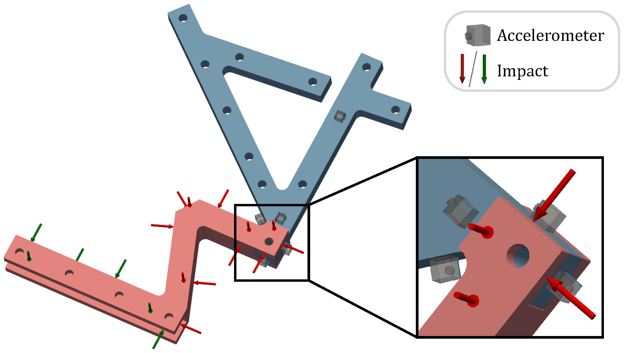
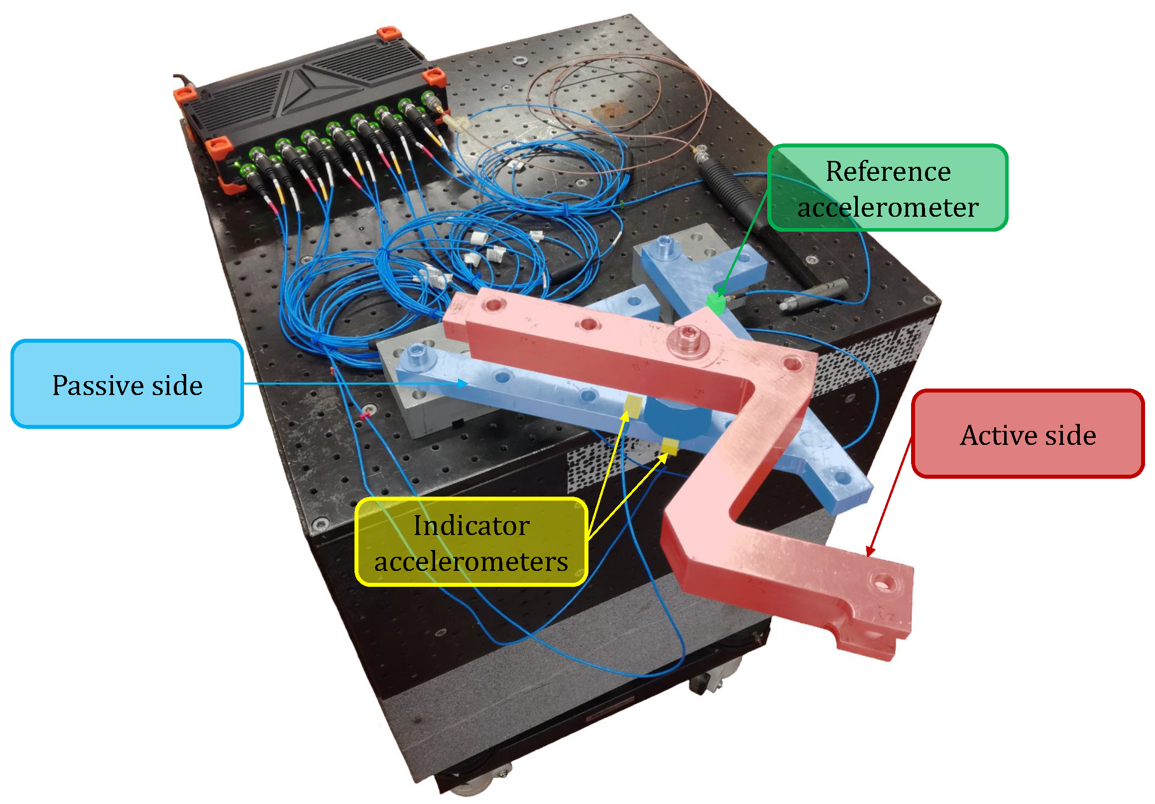
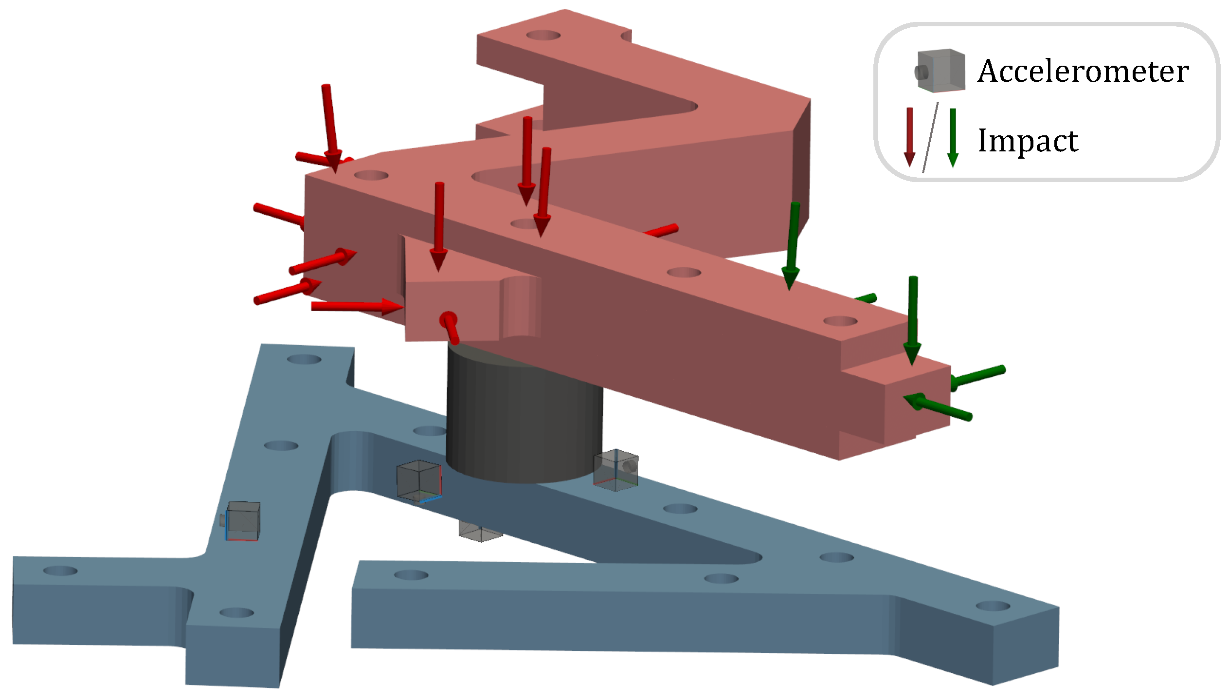
3. Experimental Case Studies

An experimental validation of the proposed method was conducted using two distinct experimental setups. The first setup involved two beam-like structures connected by two different types of connections. The first type was a bolted connection detailed in Section 3.1. The second type involved a rubber connection, where a rubber element was used to couple the two substructures, as described in Section 3.2. The third experimental validation featured an electric motor mounted to the drum of a washing machine, representing a more realistic case study. The associated experimental setup and results are presented in Section 3.3.

3.1. Bolted Connection

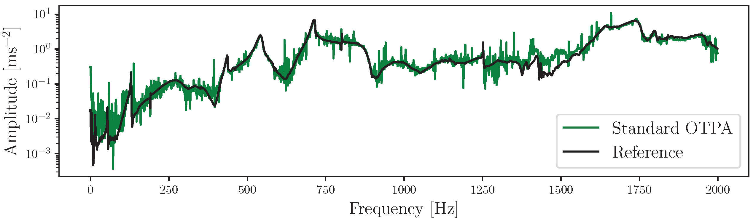
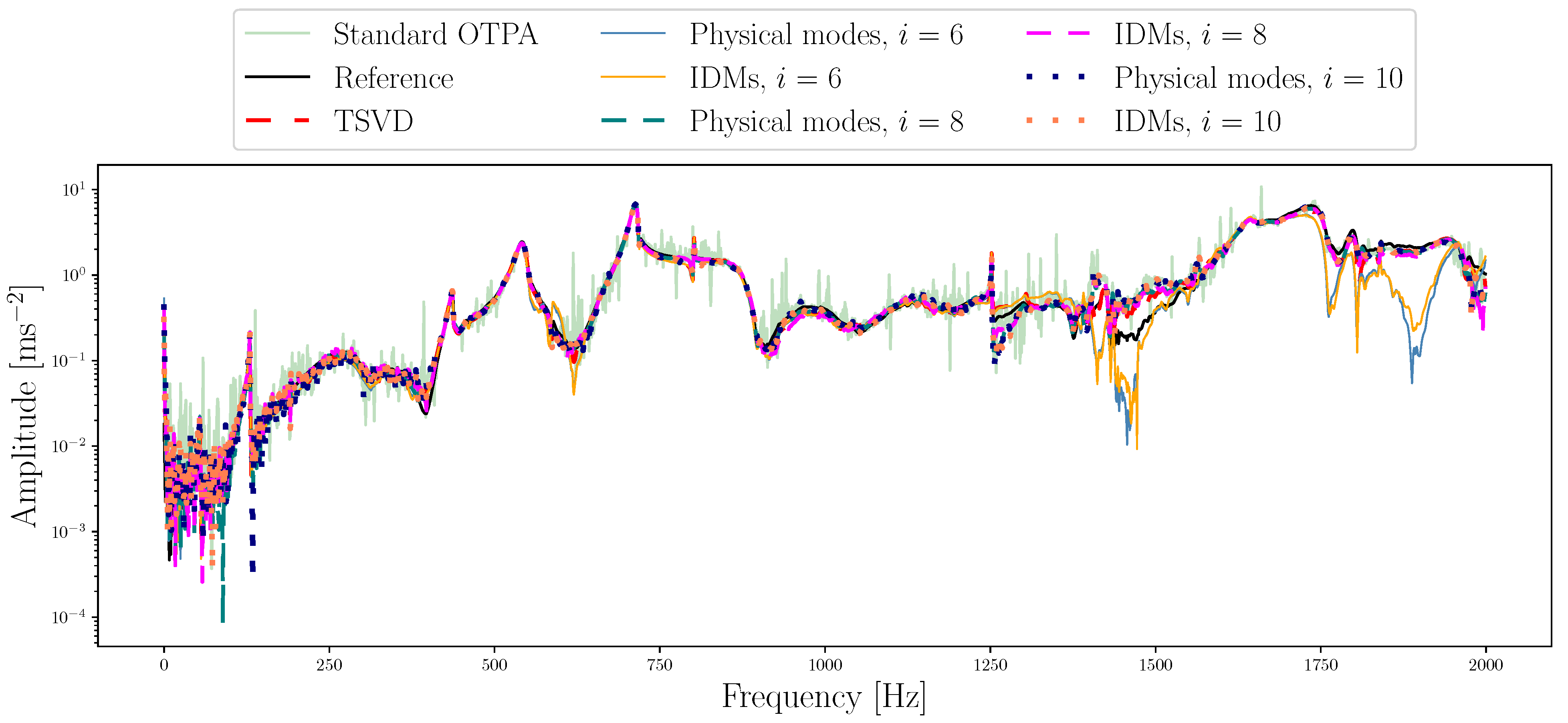
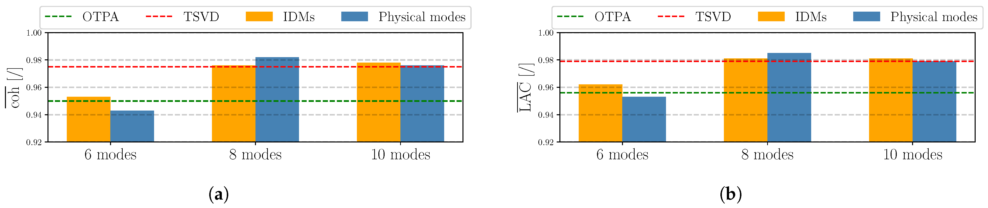
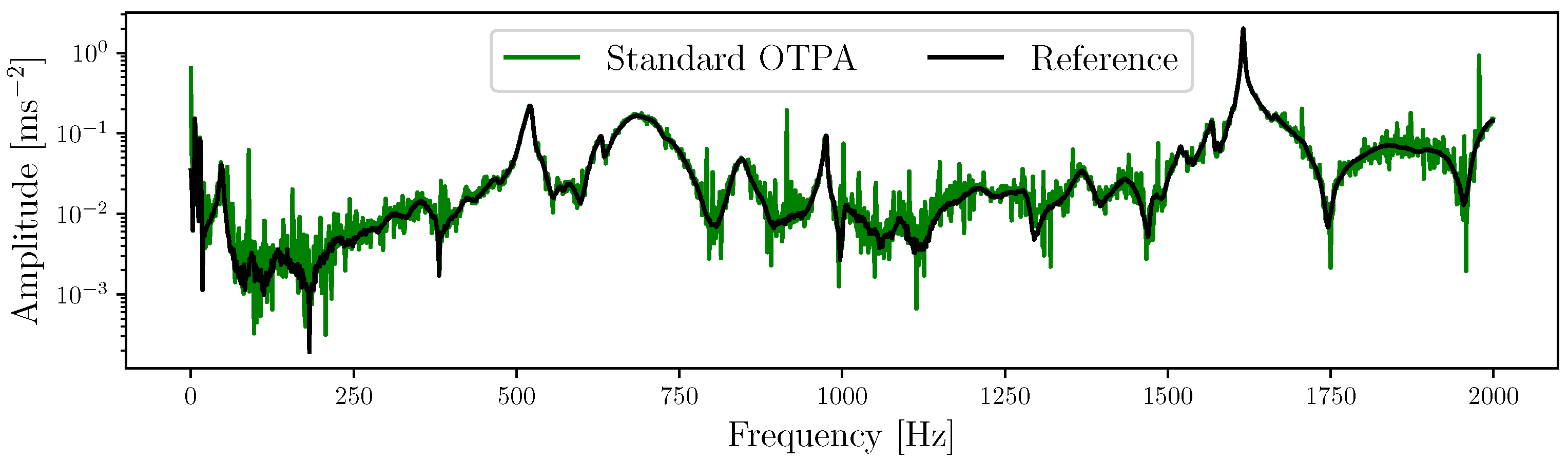
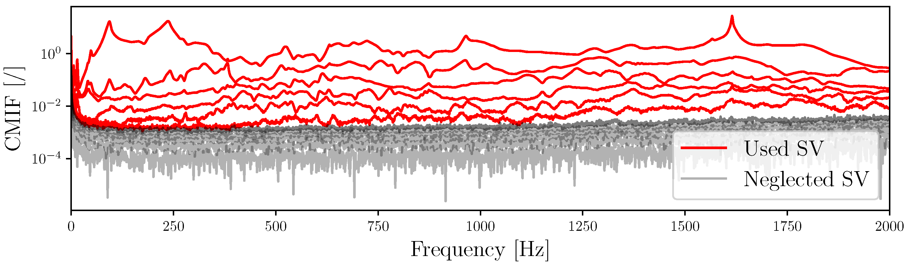
The first experimental setup consisted of an assembly of two aluminum substructures, as shown in Figure 1. A connection resembling a single point-like interface was applied to substructures A and B using an M10 bolt that was tightened with a torque of 10 Nm. The structure was securely mounted to a vibration-free table on two aluminum blocks with M10 bolts. The mass of the coupled AB structure is approximately 2.6 kg.

The response measurements were performed with five tri-axial modal PCB 356A32 accelerometers mounted on passive side B. Each accelerometer has a mass of 5 g. The first four accelerometers mounted in the vicinity of the interface acted as indicator DoFs, while the final reference accelerometer was mounted further away from the interface at the target DoFs. The positions and orientations of the accelerometers near the interface were carefully chosen to ensure sufficient observability. This was achieved by placing them on different surfaces that were perpendicular to each other. The operational excitations were simulated using a PCB 086C03 modal hammer with a vinyl tip. A total of eighteen impact/operational loads were applied to the active side. The first twelve were used in the process of estimating the transmissibility matrix (Equations (1) and (12)), while the other six were used as different load cases from which the transfer-path identification was performed following Equation (2). Figure 2 illustrates the positions and orientations of the applied impacts on active substructure A, as well as the positions of the accelerometers mounted on passive substructure B. The impact locations were chosen to ensure sufficient interface excitation. This, combined with adequate interface observability achieved through strategic accelerometer placement around the interface, enables the identification of IDMs necessary for transformation matrix construction. Unlike physical modes, which are obtained numerically, IDMs are calculated from measurements.

Results

Following Equation (2), we performed the reconstruction for the standard OTPA, which, compared to the reference measurement performed at the target DoFs ${\mathbf{u}}_3$, provides visual insight into the consistency of the method. This comparison is shown in Figure 3. All the following results in this section will be shown for the x direction of the reference accelerometer located at the target DoF ${\mathbf{u}}_3$.

From Figure 3, we can see that the standard OTPA method closely follows the reference, but it is affected by noise and spurious peaks across the entire frequency band. The noise pollution and spurious peaks can be attributed to the relatively low signal-to-noise ratio of the measurements and the high condition number (averaging well above the desired value of ${10}^2$ across the frequency range of interest [14]) of the matrix to be inverted in the process of estimating the assembly’s transferability (Equation (1)).

To apply the approach proposed within this paper, first, a numerical model of the coupled aluminum structure was constructed in ANSYS 2021 R1. The CAD models of the AB beam structure are available on the $pyFBS$ website [34]. The numerical model was constrained with a bonded connection at the interface, while a fixed support was applied at the mounting locations. A modal analysis was performed to obtain all the physical modes up to 2 kHz, which were used to construct the physical mode-transformation matrix following Equation (15). The material properties of aluminum were used (density = $2770{\displaystyle \frac{\mathrm{kg}}{{\mathrm{m}}^3}}$ and Young’s modulus = $71\mathrm{GPa}$).

To aid in the process of selecting the proper number of both physical modes and IDMs, an SVD was performed [12]. The matrix ${\mathbf{U}}_4$ can be expressed by SVD as

$${\mathbf{U}}_4=\mathbf{U}\mathsf{\Sigma }{\mathbf{V}}^{\mathrm{H}},$$

(16)

where $\mathbf{U}$ represents a $l\times l$ unitary matrix of left singular vectors, $\mathsf{\Sigma }$ is a $l\times m$ matrix containing singular values at its diagonal in descending order, $\mathbf{V}$ is a $m\times m$ unitary matrix of the right singular vectors, and superscript ${(\star )}^{\mathrm{H}}$ denotes a conjugate transpose.

This enables the creation of a graphical depiction of singular values that vary with frequency, as depicted in Figure 4.

Figure 4 demonstrates that employing six singular values, indicative of a rigid-type connection, aptly captures the interface dynamics up to approximately 1 kHz. In other words, the first six singular values dominate the interface dynamics. Incorporating more singular values makes it possible to capture the structure’s additional flexible interface behaviors, which have a larger role at higher frequencies.

To improve the prediction, the projection of the indicator responses into a sub-space following Equation (11) was applied, first with IDMs, i.e., six rigid IDMs, representing the three rotations and three translations of the interface. These IDMs provided a sufficient initial approximation of the interface dynamics, with additional flexible IDMs to be added later. For the projection with physical modes, the first six physical modes based on their corresponding natural frequency were selected as a starting point as we assume they are present within the observed frequency range.

As described previously, at the higher frequency range, additional IDMs and physical modes should be added as these represent the flexible dynamics of the interface. As such, the reduction method was also performed for a larger number of modes for both approaches to see which mode number yields the most consistent results. The proposed methods were compared to the established approach of using truncated singular-value decomposition (TSVD) in the scope of OTPA [14], where six singular values, previously determined to reflect the dynamics of the interface, were utilized and the rest were discarded. The comparison of the reconstruction of the reduction methods using IDMs and physical modes, employing six, eight, and ten modes, is illustrated in Figure 5. Specifically, for the instance of the eight-mode IDMs, an additional two extension modes [32] were incorporated. Similarly, for the ten-mode IDM case, the last remaining extension mode and an extra torsional [32] mode were included. For the approach using physical modes, the closest higher modes in terms of their corresponding natural frequency were added to construct eight- and ten-mode reduction bases.

The reconstruction presented in Figure 5 suggests that employing only six rigid IDMs or six physical modes falls short of achieving a consistent reconstruction, particularly within the frequency range from 1400 Hz to 2000 Hz. The omission of flexible motion in the reconstruction when using six rigid IDMs or physical modes resulted in a notable divergence from the reference measurements at these frequencies. Consequently, to enhance the consistency of the predictions, eight IDMs and eight physical modes were incorporated, as depicted in Figure 5, leading to a marked improvement in the prediction consistency at higher frequencies. Furthermore, the introduction of additional modes—ten IDMs and ten physical modes in total—demonstrated better consistency compared to the use of six modes. However, this also introduced a significant amount of measurement noise at lower frequencies, which is likely due to the flexible interface behavior masked by the measurement noise at these frequencies being amplified in the final prediction. Based on these observations, it was deduced that the ideal number of modes to employ for the specified frequency range is approximately eight.

For a more objective consistency estimation, the Local Amplitude Criterion LAC [35] and coherence [26] criteria were chosen. The LAC criteria make it possible to compare two frequency response functions only in terms of the amplitude, while the coherence criteria also enable the comparison in both the phase and amplitude spectra (where a value of 1 represents a perfect correlation, while values close to 0 represent poor correlations). Figure 6 displays the LAC and coherence criteria values, averaged for the entire frequency range of interest, where each depicted approach is compared to the reference measured response at the target DoF.

Figure 6 clearly indicates that the ideal number of IDMs and physical modes is eight, where both methods offered improved consistency over the standard OTPA while being comparable to the TSVD approach. The results demonstrate the importance of selecting the appropriate number of IDMs or physical modes. Similarly, the cutting point for the TSVD is up to the experimenter, which in practice is not always a trivial matter. Therefore, the use of the reduction methods using IDMs or physical modes can be viewed as a viable alternative to the TSVD approach to increase the robustness of OTPA.

3.2. Rubber Connection

The second experimental setup consisted of an assembly of two aluminium substructures, as shown in Figure 7. The coupling between substructures A and B is a rubber bushing, M10 bolts, washers, and a torque of 10 Nm. The structure is fixed to a vibration-free table on two aluminium blocks and M10 bolts tightened with a torque of 10 Nm. The mass of the coupled AB structure is 3.3 kg. It is important to note that the interface between active substructure A and passive substructure B is somewhat arbitrary and can be defined by the experimenter. In this case study, the rubber bushing was considered to be part of the passive side, but it would also be valid to include it as part of the active side.

The measurement setup included five tri-axial modal PCB 356A32 accelerometers positioned on passive side B. The initial four accelerometers were strategically placed at the interface near the rubber bushing to ensure sufficient interface observability, serving as indicator DoFs, while the fifth, a reference accelerometer, was situated further from the interface at the target DoFs. The operational excitation was simulated using a PCB 086C0 modal hammer with a vinyl tip. Operational excitation, similar to the first experimental setup, was conducted at low force levels. A total of eighteen impacts were applied on active side A at varying DoFs. The first twelve were utilized to calculate the transmissibility matrix (Equations (1) and (12)), and the subsequent six impacts were treated as different load cases to determine the path contributions, in accordance with Equation (2). Figure 8 illustrates the positions and orientations of the applied impacts on active substructure A, as well as the positions of the accelerometers mounted on passive substructure B.

Results

Figure 9 shows the comparison between the reconstructed results obtained by using the standard OTPA and the reference measurements.

From Figure 9, it is clear that the standard OTPA matches well with the reference measurements around the resonance regions of the structure where the signal-to-noise ratio is high, while elsewhere the reconstruction includes more noise and multiple spurious peaks.

A new numerical model was once again developed using ANSYS software. This model was composed of an aluminium assembly connected by a rubber element. The rubber component was represented as a cylindrical solid with dimensions of 39 mm in height and 25 mm in radius. The rubber was characterized by a linear model with a density of 1.28 ${\displaystyle \frac{\mathrm{g}}{{\mathrm{cm}}^3}}$ and a Young’s modulus of 11 MPa. Modal analysis was conducted to capture all the mode shapes up to a frequency of 2 kHz.

To determine the initial numbers of IDMs and physical modes to be utilized within their respective transformation matrices, an additional SVD was performed. The graphical illustration that compares the utilized singular values with the residual ones is shown in Figure 10.

Figure 10 reveals that six singular values can represent the interface dynamics within the observed frequency range. Accordingly, six rigid IDMs and the first six physical modes (based on their corresponding natural frequencies) were chosen to form their respective transformation matrices in line with Equations (10) and (15). However, transformation matrices for eight and ten modes were also constructed to demonstrate the consequences of employing an excessive number of IDMs or physical modes. In the configuration with eight IDMs, an additional two extension modes were incorporated, while, for the configuration with ten IDMs, the final extension mode and an extra torsional mode were included [32]. Following Equation (12), the transmissibility matrix was estimated for all the constructed transformation matrices.

The reconstructed outcomes utilizing six, eight, and ten IDMs and physical modes are evaluated against the reference measurements and the TSVD approach utilizing six singular values, shown in Figure 11.

From Figure 11, we observe that this experimental setup produced consistent reconstruction results with six rigid IDMs and six physical modes. Including additional modes only introduced redundancy into the reconstruction, as evidenced by an overall increase in the measurement noise across the frequency range. This demonstrates that adding more modes does not necessarily lead to improved consistency.

These observations were also objectively validated with the coherence and LAC criteria shown in Figure 12.

The data presented in Figure 12 confirmed the findings from the reconstructed outcomes depicted in Figure 11. It is evident that the utilization of six modes for both the rigid IDMs and physical modes yielded the most consistent results, confirming the initial number of modes selected based on the SVD, as illustrated in Figure 10. The introduction of more modes did not enhance, but rather diminished, this consistency. Employing a reduction-based strategy with an optimal mode count led to an approximate 5% improvement in consistency over the standard OTPA, aligning with the results achieved with the TSVD approach. This highlights the importance of selecting the appropriate number of modes for obtaining consistent results.

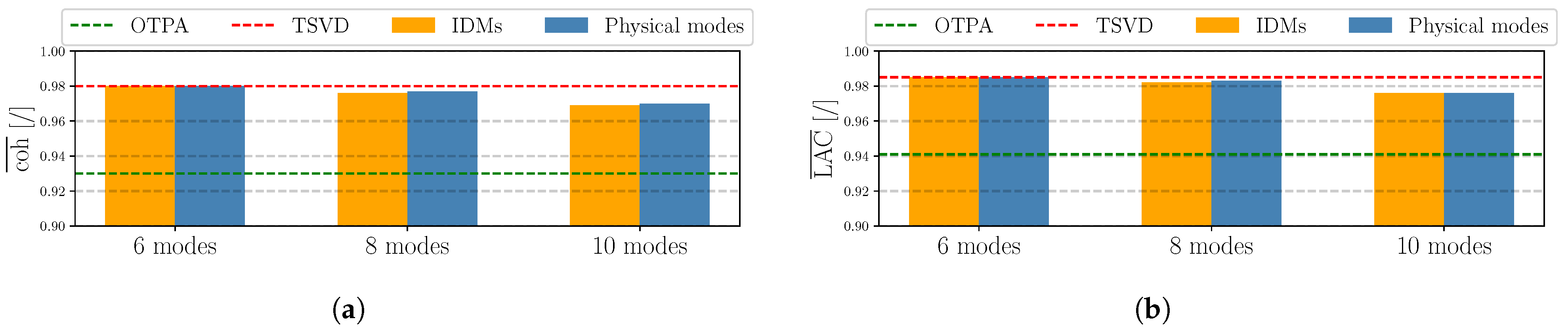
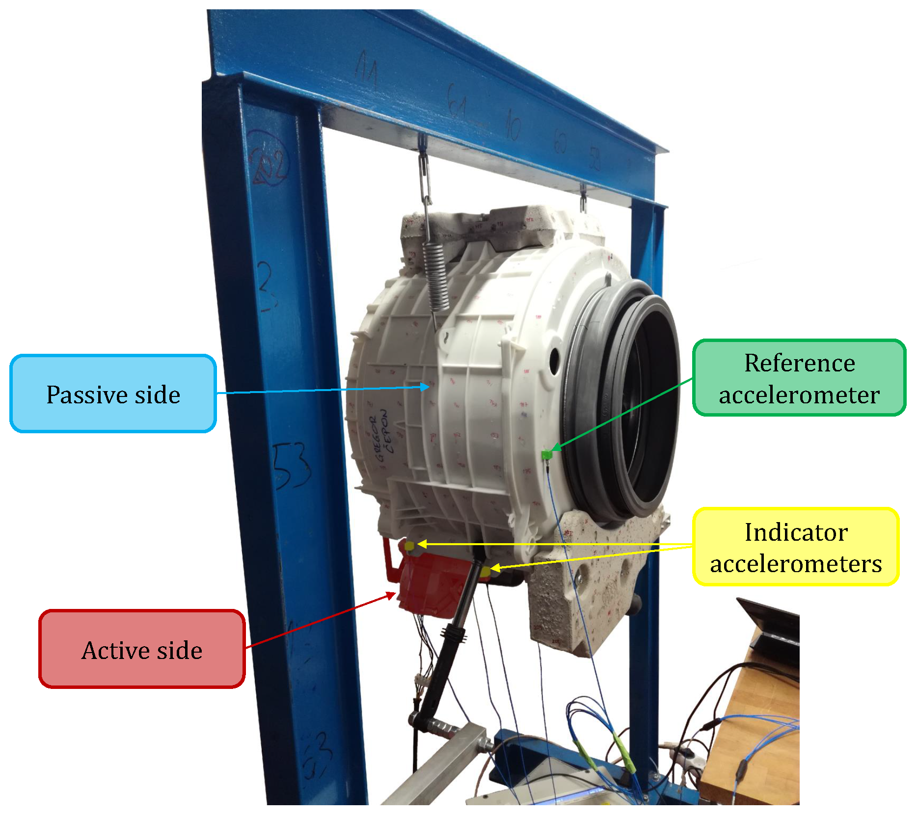
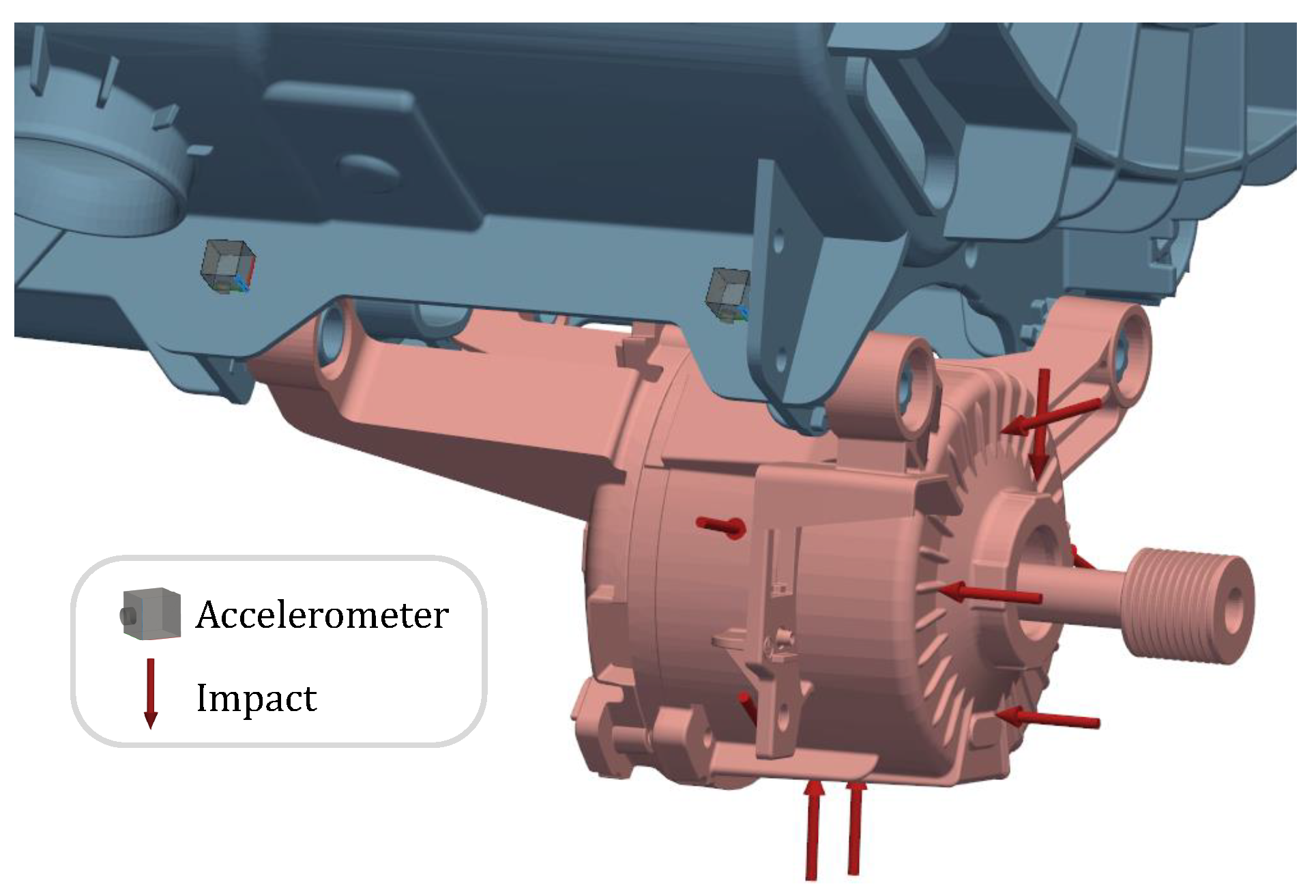
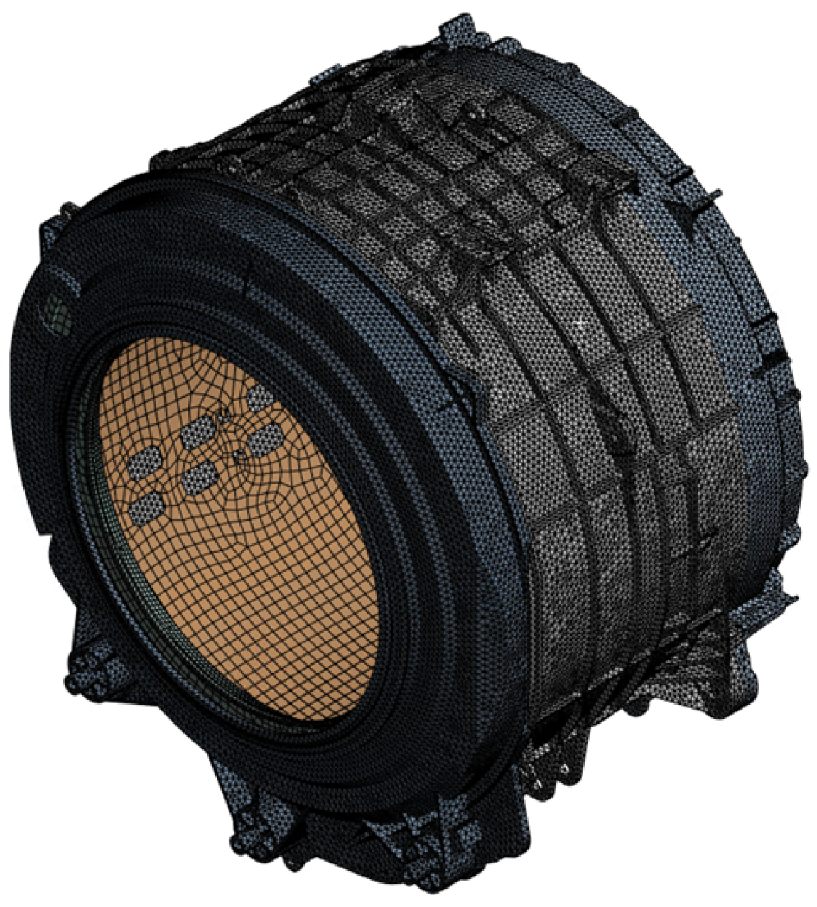
3.3. Washing Machine Drum Setup

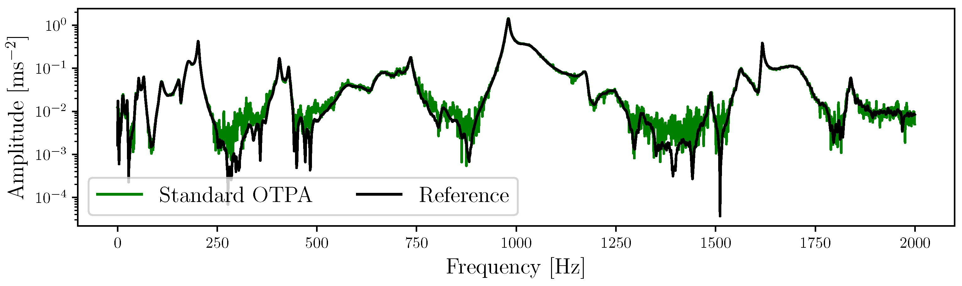
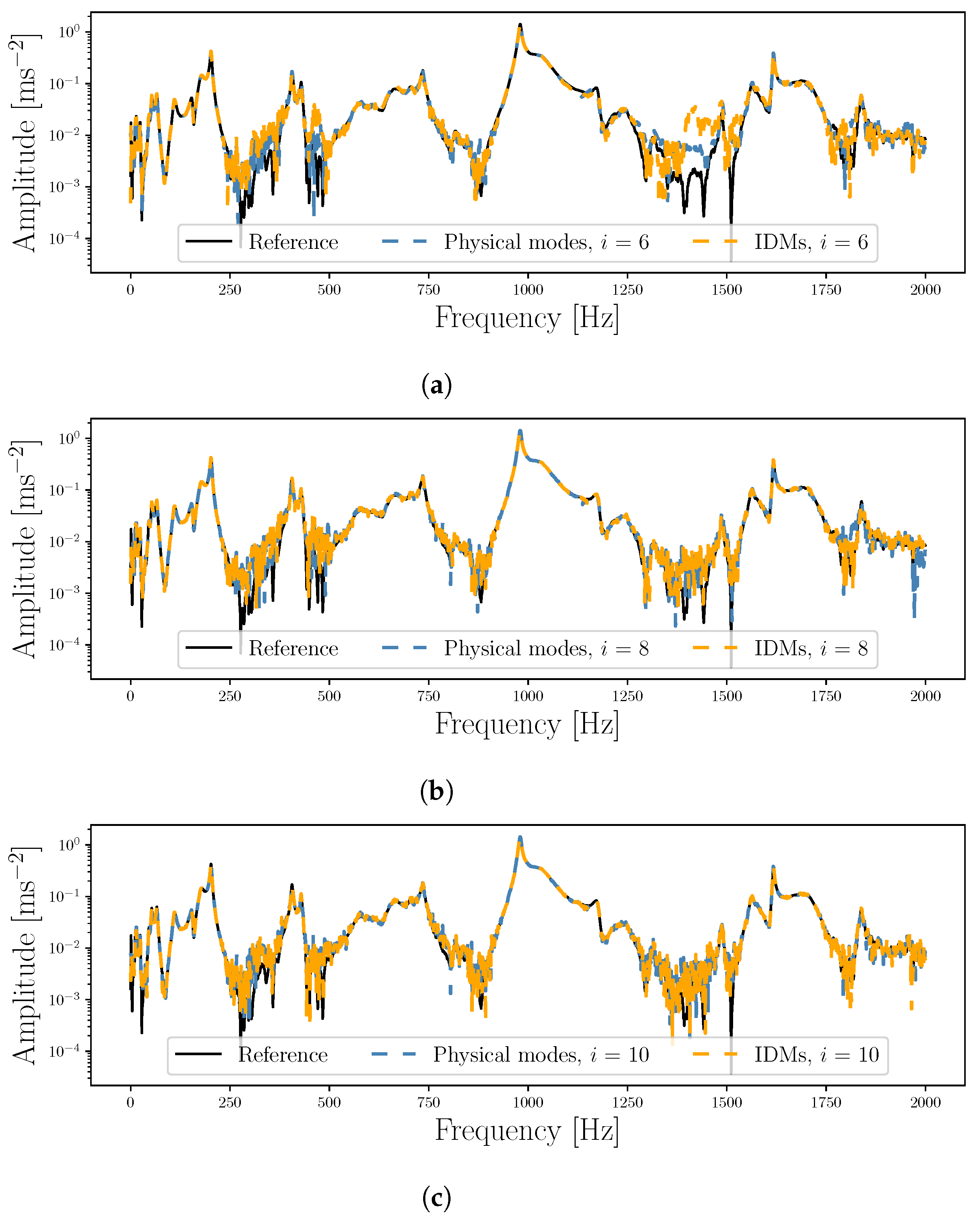
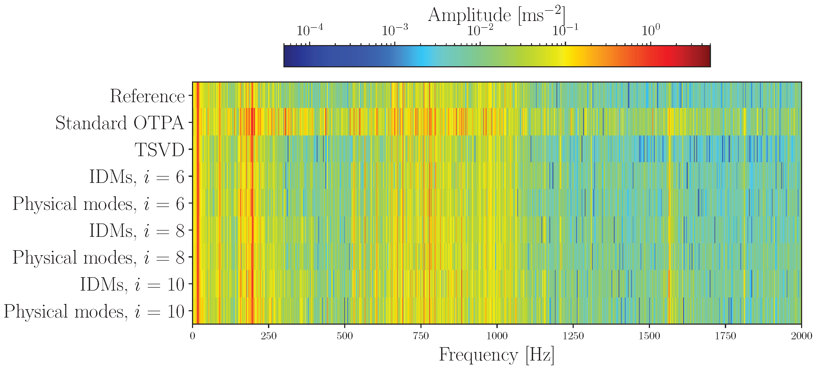
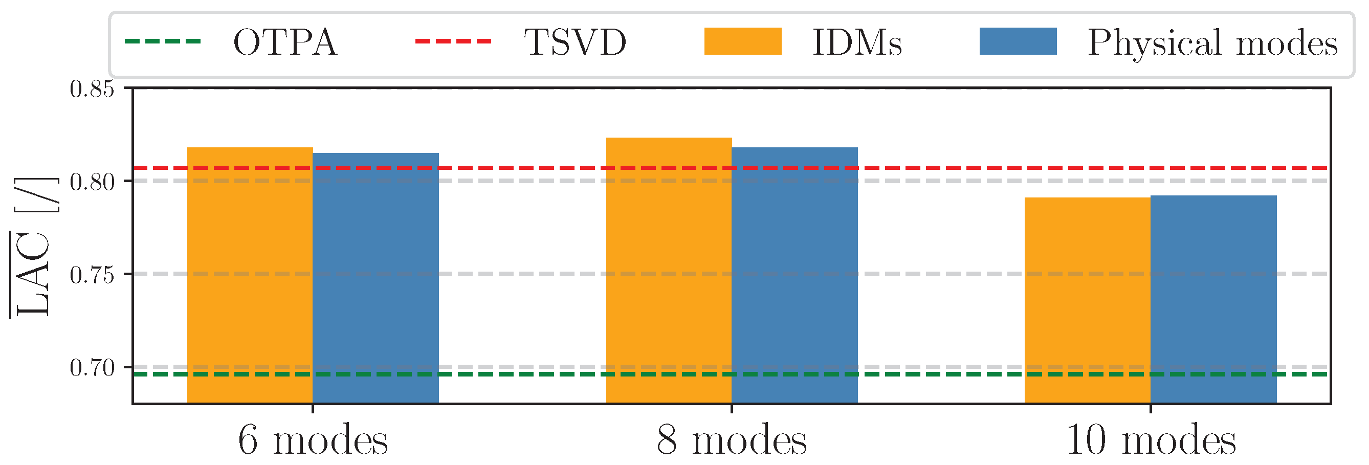
The third experimental setup involved an electric motor mounted on the drum of a washing machine, as shown in Figure 13. Inside the drum, a rotating steel drum, combined with the electric motor, served as the two sources of vibration. The drum was loaded with a uniformly distributed 12 kg mass around the drum and mounted to a dedicated steel frame with dampers and springs to simulate the conditions inside the washing machine. The combined mass of the washing machine drum assembly is around 40 kg. The goal of the measurement was to characterize the transfer of vibration from the electric motor to the washing machine drum while neglecting the secondary source, the rotating drum. This is based on the assumption that the sources mainly excite different frequency bands, i.e., lower frequency range (below 100 Hz) for the drum and higher frequency range (above 100 Hz) for the motor. Identifying the dominant transfer paths provided improved insight into where the structural modifications are needed. For example, additional vibro-isolation can decrease the vibration transfer, or drum reinforcements can increase the local rigidity, thereby reducing the dynamic response of the passive side.

Furthermore, the measurements were performed with four tri-axial PCB 356A32 modal accelerometers positioned on the drum near the electric-motor mounts (one accelerometer per mounting pin) acting as indicator DoFs, while an additional reference accelerometer was positioned at the front of the drum. The locations of indicator accelerometers were selected to achieve sufficient observability of the interface while minimizing the number of accelerometers to avoid redundant measurements from duplicated channels.. The reference location was chosen near the rubber below, which represents one of the main connection points between the washing machine drum and the machine’s enclosure when it is fully assembled. As such, high vibration on the drum would cause the whole enclosure to vibrate. To characterize the transfer paths, two measurement approaches were selected. The initial set involved conducting 18 impacts using a modal hammer on different parts of the electric motor. The subsequent set included measurements taken during the motor’s operation under 18 separate load conditions. This was accomplished by adjusting the motor’s RPM in a consistent range from 400 RPM to 1250 RPM, increasing by increments of 50 RPM. Figure 14 shows the position and orientation of the impacts applied on the motor using the modal hammer.

Results

The transmissibility matrix is estimated by following Equation (1) using the initial 12 response measurements obtained from the impacts. Subsequently, this matrix is used to reconstruct the responses at the target DoFs for the standard OTPA. The results of this reconstruction are evaluated against the reference measurements, as depicted in Figure 15.

The reconstructed results in Figure 15 closely matched the reference measurements near the peaks, where the signal-to-noise ratio was high. However, deviations occur in regions dominated by noise.

A numerical model within ANSYS was constructed, as shown in Figure 16, to obtain the physical mode shapes of the assembly. The washing machine drum and shaft were modeled as flexible solids, while the drum was modeled as a flexible shell. For the electric motor and concrete weights, rigid mass points were used with their respective mass values. An additional mass element was used for the internally applied mass of 12 kg, which was evenly distributed around the face of the drum. The two bearings were modeled using the ANSYS SKF extension, where they were designated as bearings 6206 and 6205 with a non-linear stiffness type. The drum was composed of PPCaCo3, while the remaining parts were composed of structural steel. The material parameters are detailed in

Table 1. Material parameters.

	Young’s Modulus	Density
PPCaCo3	2800 MPa	$1.0{\displaystyle \frac{\mathrm{g}}{{\mathrm{cm}}^3}}$
Structural steel	200 GPa	$7.85{\displaystyle \frac{\mathrm{g}}{{\mathrm{cm}}^3}}$

.

The comprehensive numerical model is composed of approximately 580,000 elements, predominantly Hex20. A modal analysis was ultimately conducted under a free–free boundary condition. This analysis yielded the initial twelve mode shapes, excluding the three translational and three rotational modes that result from the free–free boundary condition. These mode shapes were then utilized to create the transformation matrix of the physical modes.

Furthermore, an SVD was performed to obtain the number of dominant singular values in the interface, based upon which the numbers of IDMs and physical modes were selected. The graphical representations using six singular values are shown in Figure 17.

Figure 17 shows that six singular values do not sufficiently describe the dynamics at the interface. This is clear from the increased amplitude of the seventh singular value around 1000 Hz and also the eighth around 1500 Hz, meaning that using six modes would fulfill the rigidity requirement only up to 1000 Hz, while, for higher frequencies, the inclusion of flexible modes is required.

In an effort to enhance the consistency of the reconstruction, the reduction method we proposed, which is based on IDMs and physical modes, was employed once more. Transformation matrices were constructed for the cases using six rigid, eight, and ten IDMs or physical modes. Specifically, for the six rigid IDMs case, three translational and three rotational modes were incorporated; for eight IDMs, two additional extension modes were included; and, for ten IDMs, one more extension mode along with an extra torsional mode were added [32]. Moreover, the transmissibility matrix was estimated (Equation (12)) for each separate transformation matrix. The reconstructed results, derived from Equation (13), were compared with the reference measurements (Figure 18).

Figure 18 demonstrates that utilizing more than six rigid IDMs or physical modes resulted in more consistent reconstructions. The most notable improvement was observed around 1300 Hz, where the use of only six modes led to subpar consistency. In contrast, employing either eight or ten modes enhanced the consistency. However, the application of ten modes began to introduce redundancy, as indicated by the increased noise present within the reconstructed results compared to using eight modes. Consequently, for this case study, eight IDMs and physical modes were identified as being optimal and will be further validated in the upcoming measurement campaign.

The same approach was then applied in an operational test. Here, the excitation source was the electric motor running at a steady speed. The distinct load cases were established by altering the motor’s RPM from 400 to 1250, in increments of 50 RPM. This resulted in eighteen different load cases. The first twelve cases were utilized to estimate the transmissibility matrix, while the remaining six were employed in the reconstruction process, in accordance with Equation (13). Following the conclusion of the previous measurements, transformation matrices for the IDMs and the physical modes were constructed using eight modes. However, to validate this conclusion, additional transformation matrices using six and ten IDMs and physical modes were also constructed, where the IDMs that were used in the construction of the transformation matrix again consisted of translational, rotational, extension, and torsion modes. The reconstructions for the six, eight, and ten IDMs or physical modes were compared to the standard OTPA and the TSVD approach, where, for the TSVD approach, a cutting point set at eight singular values was used. Comparisons using their respective number of modes are shown in Figure 19.

From Figure 19, it is clear that the reconstruction using standard OTPA shows a higher amplitude over the whole frequency range compared to the others. This was attributed to redundant responses and consequent poor conditioning of the ${\mathbf{U}}_4$, which caused the amplification of measurement noise. Nonetheless, the implementation of reduction methods improved the consistency of the reconstructions compared to the standard OTPA, yielding results that are comparable to those obtained with the TSVD technique. However, it is difficult to determine the optimal number of IDMs and physical modes to obtain the most consistent results based solely on Figure 19. Therefore, a more objective measurement is used, i.e., the LAC criteria In this instance, only the LAC criteria were selected because they provide an objective measure for comparing amplitudes. The coherence criteria were considered to be unsuitable as they account for the phase as well, which was random across much of the frequency spectrum. The average LAC values obtained are shown in Figure 20.

Figure 20 shows that the incorporation of physical modes or IDMs into the reduction-based method enhanced the consistency of OTPA. For six, eight, and ten IDMs or physical modes, a marked enhancement is evident when compared to the standard OTPA. It also presented a modest improvement over the TSVD approach for scenarios involving six and eight modes, although the results for ten modes were not as favorable. Nevertheless, an approximate 12% improvement was achieved over the standard OTPA when utilizing eight IDMs or physical modes, concluding that the optimal number of utilized IDMs and physical modes is eight. Confirming the appropriate number of modes to use by performing the SVD, it was determined that using six modes was insufficient to fully describe the interface dynamics across the observed frequency range, especially at higher frequencies.

Given that the primary objective of OTPA is to identify the dominant transfer paths, we examined the impact of employing reduction-based methods on this process. Utilizing Equation (4), we determined the path contributions for the standard OTPA, the TSVD approach, and both reduction-based methods, selecting eight as the number of IDMs and physical modes. The partial path contributions are shown in Figure 21.

The data presented in Figure 21 reveal that the standard OTPA displayed higher amplitudes across the frequency spectrum, a result of poor conditioning of ${\mathbf{U}}_4$ and consequent noise amplification, unlike the other three methods. The reduction-based methods provided a more pronounced separation of the excited frequencies. While the TSVD method demonstrated similar clarity at lower frequencies, its effectiveness diminished amidst the noise at higher frequencies. In contrast, the two methods based on reduction maintained their performance at these higher frequencies, which can be attributed to the inclusion of flexible modes.

4. Conclusions

This paper introduced a reduction-based approach to improve the consistency of partial path-contribution estimations in operational transfer-path analysis. By projecting measured operational responses onto representative sub-spaces constructed from interface-deformation modes and physical modes, partial path predictions were obtained by considering only the important interface dynamics, while the rest were left unobserved. By neglecting poorly observed and redundant interface dynamics, the transmissibility-matrix estimation for OTPA can become more robust, addressing key issues such as noise amplification and the ill-conditioning of the inverse problem.

The experimental validation, conducted across setups including bolted and rubber-coupled beam structures as well as a washing machine drum assembly, demonstrated the proposed method’s effectiveness. The experimental results showed that using appropriate numbers of IDMs and physical modes led to improvements in the path-contribution estimations, particularly in reducing noise amplification. However, it was observed that the consistency of the method diminished in the higher frequency range when either too many or too few modes were used. This could be considered a limitation of the method, particularly in cases where the appropriate number of IDMs cannot be measured due to poor observability or excitation at high frequencies. These findings suggest that the reduction-based approach offers a viable alternative to conventional regularization techniques such as truncated singular-value decomposition, but they also provide insight into the interface dynamics (i.e., the number and type of significant interface DoFs). However, it should be noted that the selection of modes in the reduction step by the experimenter plays a crucial role in the effectiveness of the proposed methods. Therefore, when studying large and complex structures with multiple varying connection types, where constructing a representative numerical model requires significant effort, it is recommended to employ the reduction approach solely using IDMs.

References

1. Verheij, J.W. Multi-Path Sound Transfer from Resiliently Mounted Shipboard Machinery: Experimental Methods for Analyzing and Improving Noise Control. Ph.D. Thesis, TU Delft, Delft University of Technology, Delft, The Netherlands, 1982. [Google Scholar]
2. Kong, L.; Zhao, X.; Yuan, X.; Yu, Q.; Shi, P.; Zhou, C.; Zhang, D. A novel vibration transfer path analysis for electric vehicle driving motor controllers under strong signal crosstalk. Mech. Syst. Signal Process. 2025, 223, 111919. [Google Scholar] [CrossRef]
3. Zheng, X.; Wang, Z.; Zhou, Q.; Hao, Z.; Qiu, Y. A study on the hybrid FE-experimental analysis method for dash panel response excited by the brake booster based on BF-TPA. Measurement 2021, 172, 108854. [Google Scholar] [CrossRef]
4. Liu, Z.; Gao, D.; Gao, Y.; Yang, J. Numerical and experimental-aided framework based on TPA for acoustic contributions of individual transfer paths on a vehicle door in the slamming event. Appl. Acoust. 2023, 203, 109220. [Google Scholar] [CrossRef]
5. Hou, L.; Cao, S.; Gao, T.; Wang, S. Vibration signal model of an aero-engine rotor-casing system with a transfer path effect and rubbing. Measurement 2019, 141, 429–441. [Google Scholar] [CrossRef]
6. El Khatiri, W.; Cherif, R.; El Bikri, K.; Atalla, N. Experimental study of component-based transfer path analysis hybrid methods applied to a helicopter. Appl. Acoust. 2023, 210, 109431. [Google Scholar] [CrossRef]
7. Prenant, S.; Padois, T.; Rolland, V.; Etchessahar, M.; Dupont, T.; Doutres, O. Effects of mobility matrices completeness on component-based transfer path analysis methods with and without substructuring applied to aircraft-like components. J. Sound Vib. 2023, 547, 117541. [Google Scholar] [CrossRef]
8. Li, C.; Lu, P.; Chen, G. VNCCD: A gearbox fault diagnosis technique under nonstationary conditions via virtual decoupled transfer path. Mech. Syst. Signal Process. 2024, 221, 111741. [Google Scholar] [CrossRef]
9. Liu, C.; Zhang, Y.H.; Zhang, X.Z.; Zhang, Y.B.; Chen, L.Q. Source contribution analysis of vehicle pass-by noise using a moving multi-band model based OPAX method. Measurement 2023, 218, 113170. [Google Scholar] [CrossRef]
10. van der Seijs, M.V.; de Klerk, D.; Rixen, D.J. General framework for transfer path analysis: History, theory and classification of techniques. Mech. Syst. Signal Process. 2016, 68–69, 217–244. [Google Scholar] [CrossRef]
11. Mondot, J.; Petersson, B. Characterization of structure-borne sound sources: The source descriptor and the coupling function. J. Sound Vib. 1987, 114, 507–518. [Google Scholar] [CrossRef]
12. de Klerk, D.; Rixen, D. Component transfer path analysis method with compensation for test bench dynamics. Mech. Syst. Signal Process. 2010, 24, 1693–1710. [Google Scholar] [CrossRef]
13. Elliott, A.; Moorhouse, A.; Huntley, T.; Tate, S. In-situ source path contribution analysis of structure borne road noise. J. Sound Vib. 2013, 332, 6276–6295. [Google Scholar] [CrossRef]
14. de Klerk, D.; Ossipov, A. Operational transfer path analysis: Theory, guidelines and tire noise application. Mech. Syst. Signal Process. 2010, 24, 1950–1962. [Google Scholar] [CrossRef]
15. Gajdatsy, P.; Janssens, K.; Desmet, W.; Van der Auweraer, H. Application of the transmissibility concept in transfer path analysis. Mech. Syst. Signal Process. 2010, 24, 1963–1976. [Google Scholar] [CrossRef]
16. Janssens, K.; Gajdatsy, P.; Gielen, L.; Mas, P.; Britte, L.; Desmet, W.; Van der Auweraer, H. OPAX: A new transfer path analysis method based on parametric load models. Mech. Syst. Signal Process. 2011, 25, 1321–1338. [Google Scholar] [CrossRef]
17. van der Seijs, M.V. Experimental Dynamic Substructuring: Analysis and Design Strategies for Vehicle Development. Ph.D. Thesis, Delft University of Technology, Delft, The Netherlands, 2016. [Google Scholar]
18. Aragonès, À.; Poblet-Puig, J.; Arcas, K.; Rodríguez, P.V.; Magrans, F.X.; Rodríguez-Ferran, A. Experimental and numerical study of Advanced Transfer Path Analysis applied to a box prototype. Mech. Syst. Signal Process. 2019, 114, 448–466. [Google Scholar] [CrossRef]
19. Gajdatsy, P.; Janssens, K.; Gielen, L.; Mas, P. Critical assessment of operational path analysis: Effect of coupling between path inputs. J. Acoust. Soc. Am. 2008, 123, 5821–5826. [Google Scholar] [CrossRef]
20. Roozen, N.; Leclère, Q. On the use of artificial excitation in operational transfer path analysis. Appl. Acoust. 2013, 74, 1167–1174. [Google Scholar] [CrossRef]
21. Cheng, W.; Chu, Y.; Chen, X.; Zhou, G.; Blamaud, D.; Lu, J. Operational transfer path analysis with crosstalk cancellation using independent component analysis. J. Sound Vib. 2020, 473, 115224. [Google Scholar] [CrossRef]
22. Cheng, W.; Chu, Y.; Lu, J.; Song, C.; Chen, X.; Zhang, L.; Wajid, B.A.; Gao, L. A customized scheme of crosstalk cancellation for operational transfer path analysis and experimental validation. J. Sound Vib. 2021, 515, 116506. [Google Scholar] [CrossRef]
23. Cheng, W.; Lu, Y.; Zhang, Z. Tikhonov regularization-based operational transfer path analysis. Mech. Syst. Signal Process. 2016, 75, 494–514. [Google Scholar] [CrossRef]
24. Tang, Z.; Zan, M.; Zhang, Z.; Xu, Z.; Xu, E. Operational transfer path analysis with regularized total least-squares method. J. Sound Vib. 2022, 535, 117130. [Google Scholar] [CrossRef]
25. Choi, H.G.; Thite, A.N.; Thompson, D.J. Comparison of methods for parameter selection in Tikhonov regularization with application to inverse force determination. J. Sound Vib. 2007, 304, 894–917. [Google Scholar] [CrossRef]
26. van der Seijs, M.V.; van den Bosch, D.D.; Rixen, D.J.; de Klerk, D. An improved methodology for the virtual point transformation of measured frequency response functions in dynamic substructuring. In Proceedings of the 4th ECCOMAS Thematic Conference on Computational Methods in Structural Dynamics and Earthquake Engineering, Kos Island, Greece, 12–14 June 2013; Volume 4. [Google Scholar]
27. Allen, M.S.; Mayes, R.L.; Bergman, E.J. Experimental modal substructuring to couple and uncouple substructures with flexible fixtures and multi-point connections. J. Sound Vib. 2010, 329, 4891–4906. [Google Scholar] [CrossRef]
28. Wernsen, M.; Van der Seijs, M.; Klerk, D. An indicator sensor criterion for in-situ characterisation of source vibrations. In Proceedings of the IMAC XXXV: 35th International Modal Anaylsis Conference, Los Angeles, CA, USA, 30 January–2 February 2017. [Google Scholar]
29. Allen, M.S.; Rixen, D.; Van der Seijs, M.; Tiso, P.; Abrahamsson, T.; Mayes, R.L. Substructuring in Engineering Dynamics: Emerging Numerical and Experimental Techniques; Springer: Cham, Switzerland, 2019; Volume 594. [Google Scholar]
30. Ocepek, D.; Trainotti, F.; Čepon, G.; Rixen, D.J.; Boltežar, M. On the experimental coupling with continuous interfaces using frequency based substructuring. Mech. Syst. Signal Process. 2024, 217, 111517. [Google Scholar] [CrossRef]
31. Häußler, M.; Rixen, D.J. Optimal Transformation of Frequency Response Functions on Interface Deformation Modes. In Dynamics of Coupled Structures, Volume 4; Springer: Cham, Switzerland, 2017. [Google Scholar]
32. Pasma, E.; Seijs, M.v.d.; Klaassen, S.; Kooij, M.v.d. Frequency based substructuring with the virtual point transformation, flexible interface modes and a transmission simulator. In Dynamics of Coupled Structures, Volume 4: Proceedings of the 36th IMAC, A Conference and Exposition on Structural Dynamics 2018; Springer: Cham, Switzerland, 2018; pp. 205–213. [Google Scholar]
33. Almirón, J.O.; Bianciardi, F.; Desmet, W. Flexible interface models for force/displacement field reconstruction applications. J. Sound Vib. 2022, 534, 117001. [Google Scholar] [CrossRef]
34. Bregar, T.; Mahmoudi, A.E.; Kodrič, M.; Ocepek, D.; Trainotti, F.; Pogačar, M.; Göldeli, M.; Čepon, G.; Boltežar, M.; Rixen, D.J. pyFBS: A Python package for Frequency Based Substructuring. J. Open Source Softw. 2022, 7, 3399. [Google Scholar] [CrossRef]
35. Zang, C.; Grafe, H.; Imregun, M. Frequency–domain criteria for correlating and updating dynamic finite element models. Mech. Syst. Signal Process. 2001, 15, 139–155. [Google Scholar] [CrossRef]
Figure 1. Experimental setup of the AB structure with a bolted connection.
Applmech 06 00013 g001
Figure 2. Impacts and accelerometers positioned on a CAD model of structure AB ( utilized in transmissibility matrix calculation;  different load cases).
Applmech 06 00013 g002
Figure 3. Comparison of the reconstructed standard OTPA results and the reference measurements.
Applmech 06 00013 g003
Figure 4. Representation of the first 6 singular values for the rigid connection experiment.
Applmech 06 00013 g004
Figure 5. Comparison of the reference measurements and reconstructed results of OTPA, TSVD, and reduction methods utilizing 6, 8, and 10 IDMs and physical modes.
Applmech 06 00013 g005
Figure 6. Comparison of reduction methods’ consistency compared to standard OTPA and TSVD results using various numbers of modes obtained with coherence and LAC criteria: (a) average coherence values; (b) average LAC values.
Applmech 06 00013 g006
Figure 7. Experimental setup of the AB structure with a rubber connection.
Applmech 06 00013 g007
Figure 8. Impacts and accelerometers positioned on a CAD model of structure AB coupled with a rubber bushing ( utilized in transmissibility matrix calculation; different load cases).
Applmech 06 00013 g008
Figure 9. Comparison of the reconstructed standard OTPA results and reference measurements.
Applmech 06 00013 g009
Figure 10. Representation of the first 6 singular values for the rubber connection experiment.
Applmech 06 00013 g010
Figure 11. Comparison of the reference measurements and reconstructed results of OTPA, TSVD, and the reduction methods utilizing 6, 8, and 10 IDMs and physical modes.
Applmech 06 00013 g011
Figure 12. Reduction methods’ consistency comparison to standard OTPA and TSVD results using various numbers of modes obtained with coherence and LAC criteria: (a) average coherence values; (b) average LAC values.
Applmech 06 00013 g012
Figure 13. Experimental setup consisting of the electric motor mounted on the drum of a washing machine.
Applmech 06 00013 g013
Figure 14. Impacts and accelerometers positioned on CAD model of the motor and drum.
Applmech 06 00013 g014
Figure 15. Comparison of the reconstructed standard OTPA results and reference measurements for tub assembely.
Applmech 06 00013 g015
Figure 16. Washing machine numerical model.
Applmech 06 00013 g016
Figure 17. Representation of the first 6 singular values for the drum assembly experiment.
Applmech 06 00013 g017
Figure 18. Comparison of the reference measurements and reconstructed results of reduction-based methods utilizing various numbers of modes: (a) 6 rigid IDMs and first 6 physical modes; (b) 8 IDMs and first 8 physical modes; (c) 10 IDMs and first 10 physical modes.
Applmech 06 00013 g018
Figure 19. Comparison of the reference measurements and reconstructed results for OTPA, TSVD, and reduction methods utilizing 6, 8, and 10 IDMs and physical modes.
Applmech 06 00013 g019
Figure 20. Average LAC values of the standard OTPA, TSVD, and the reduction methods using various numbers of modes.
Applmech 06 00013 g020
Figure 21. Path contributions of the respective OTPA methods: (a) standard OTPA; (b) TSVD; (c) first 8 physical modes; (d) first 8 IDMs.
Applmech 06 00013 g021aApplmech 06 00013 g021b