Analysis of Thermal Aspect in Hard Turning of AISI 52100 Alloy Steel Under Minimal Cutting Fluid Environment Using FEM


 ,
,  , , and
Abstract
1. Introduction
- To develop an integrated FEM model that incorporates both cutting parameters and cutting fluid application parameters to study thermal behaviour in hard turning process.
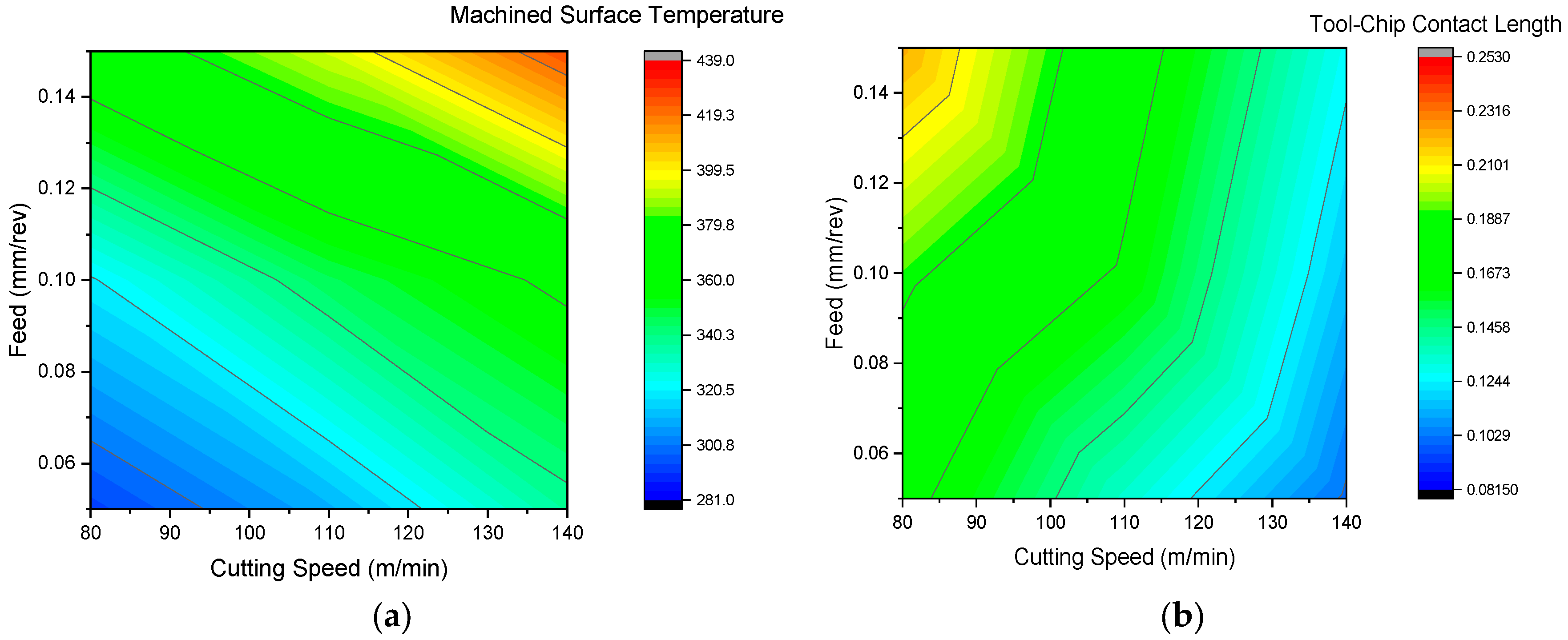
- To analyse the effect of cutting parameters and cutting fluid application parameters on cutting force, cutting temperature, machined-surface temperature and too–chip contact length during the hard turning of AISI 52100 alloy steel using the FEM.
- To validate FEM predictions with experimental results to ensure the reliability of thermal modelling for industrial applications.
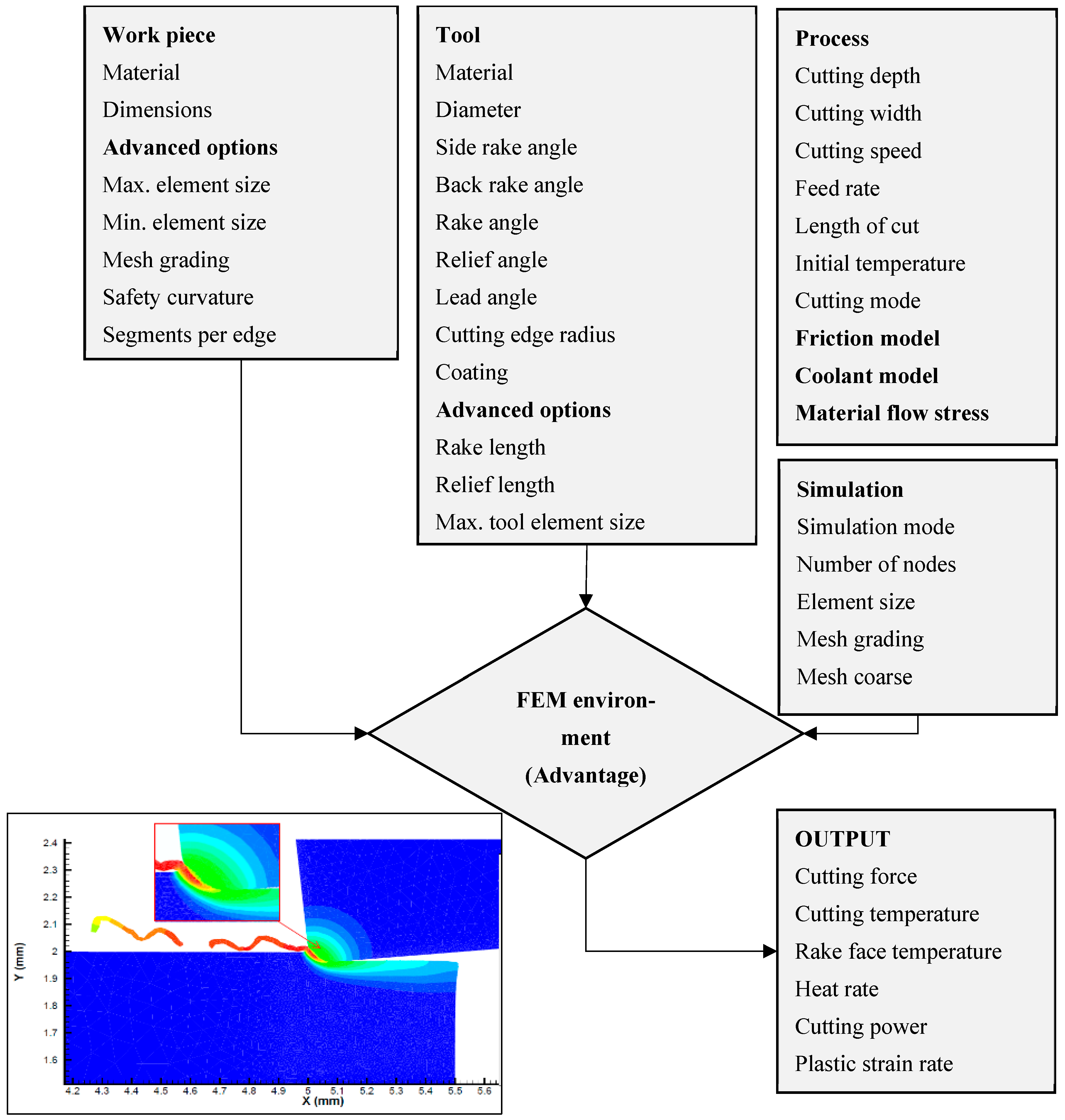
- Currently, metal-cutting simulations are performed with software like ABAQUS, DEFORM, and AdvantEdge. An effort has been undertaken to study the thermal aspect with respect to cutting temperature, machined-surface temperature, tool–chip contact length, and cutting forces in hard turning at different cutting and cutting fluid application parameters using the FEM.
2. Materials and Methods
2.1. Material Constitutive Model
2.2. Friction Modelling
2.3. Tool Modelling
2.4. Thermal Boundary Conditions
2.5. Coolant Modelling
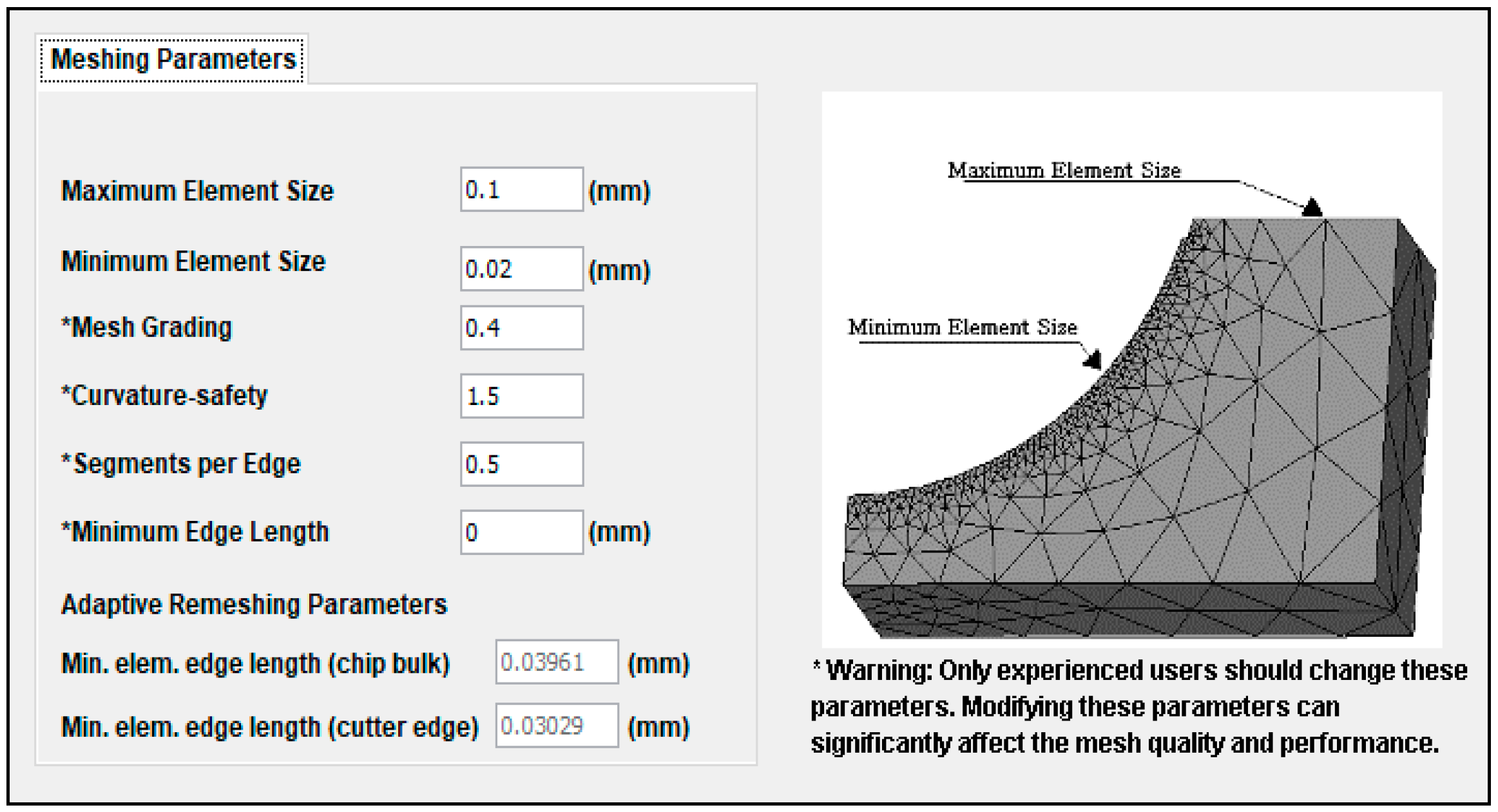
2.6. Mesh Refinement
2.7. Experimental Method
2.7.1. Test Specimen and Its Chemical Composition
2.7.2. Heat Treatment of Workpiece Material
2.7.3. Cutting Insert and Tool Holder
2.7.4. Measurement of Cutting Force
2.7.5. Cutting Fluid and Cutting Fluid Application Techniques
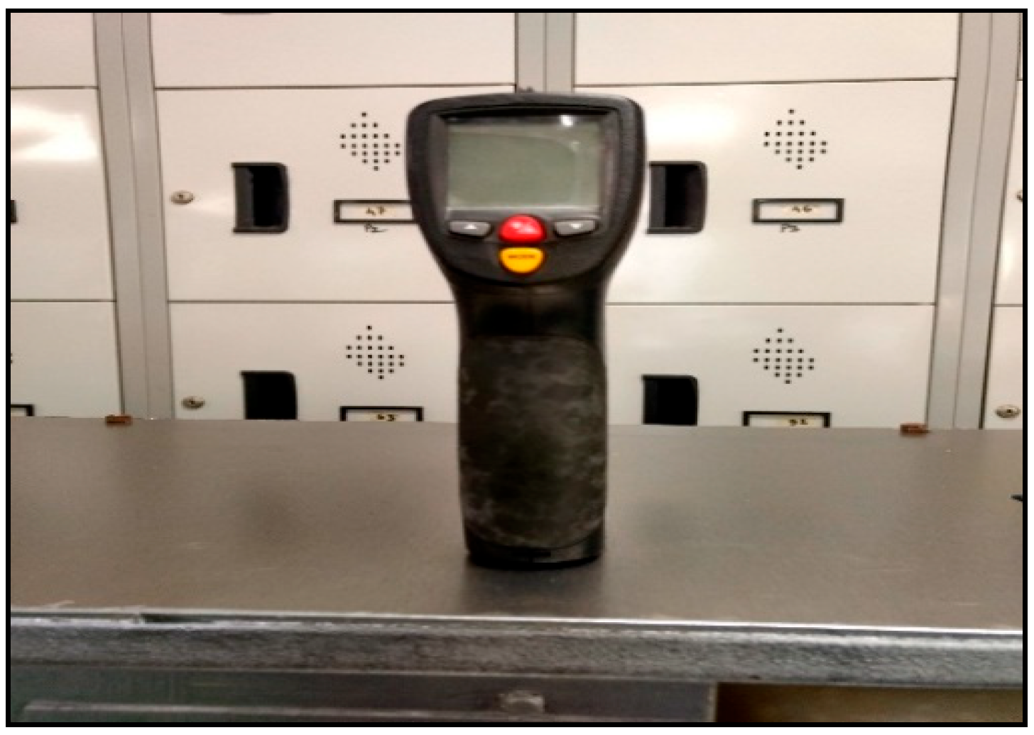
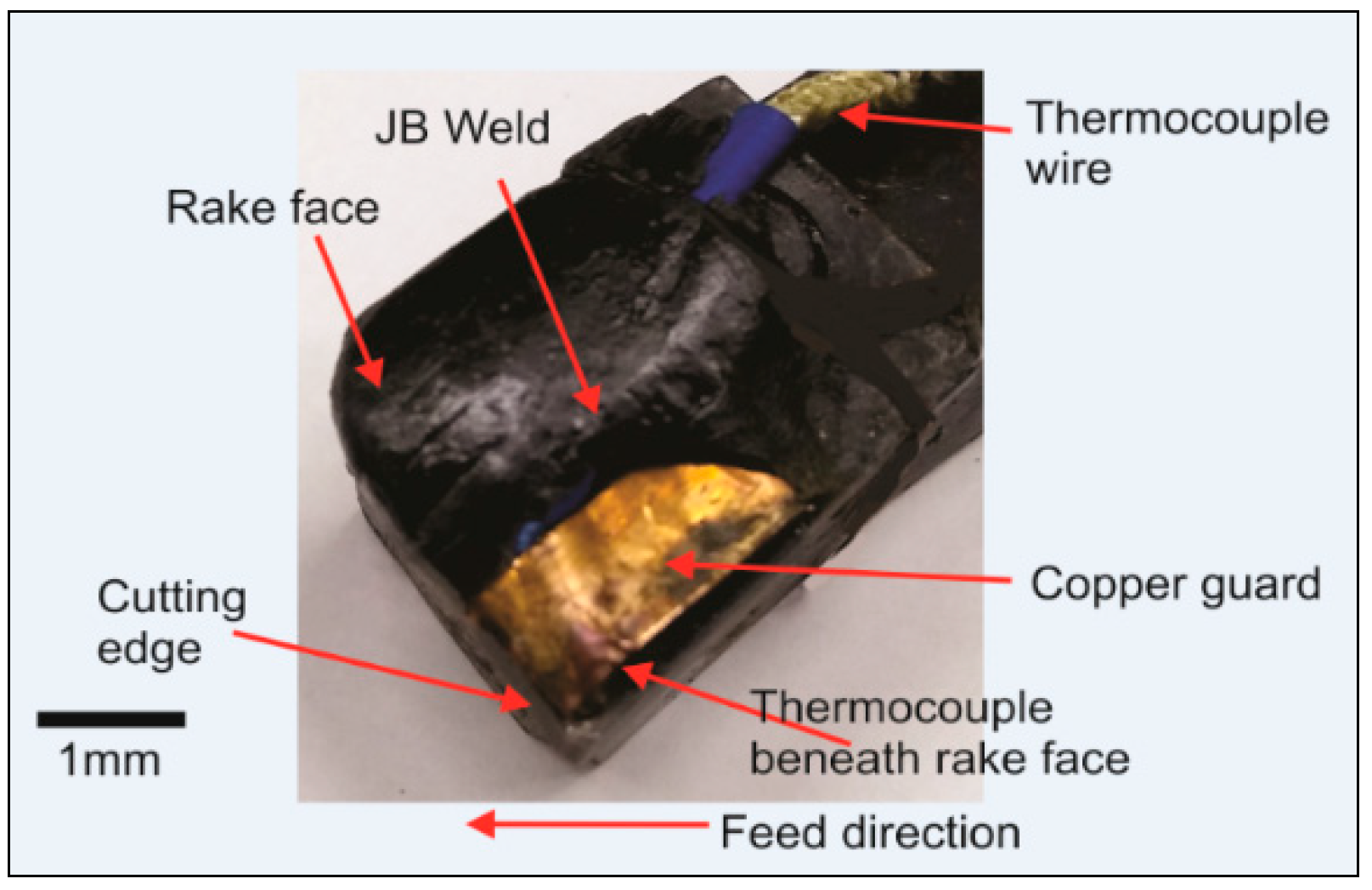
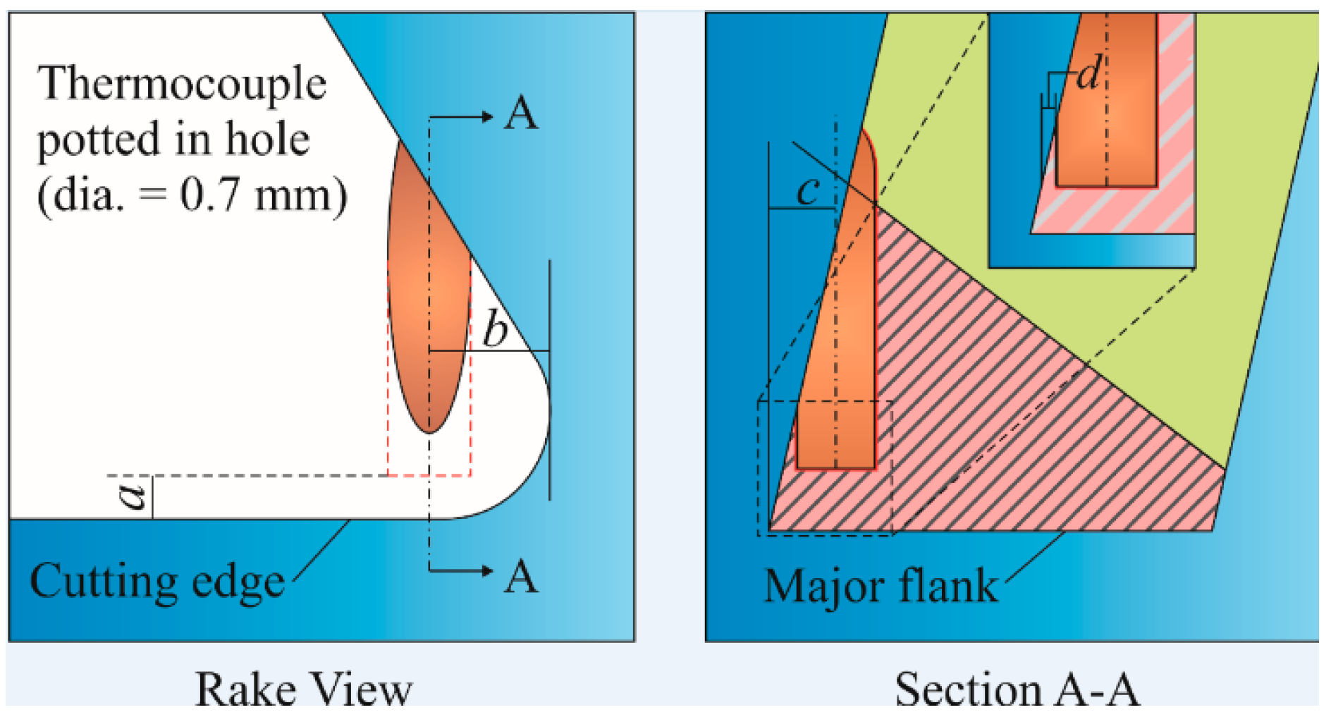
2.7.6. Measurement of Cutting Temperature
2.8. Machining Conditions
3. Result and Discussion
4. Model Validation
5. Conclusions
Author Contributions
Funding
Institutional Review Board Statement
Informed Consent Statement
Data Availability Statement
Conflicts of Interest
Abbreviations
| Annexure I | ||
| Acronyms | ||
| FEM | Finite element method | |
| CFD | Computational Fluid Dynamics | |
| FEA | Finite element analysis | |
| AISI | American Iron and Steel Institute | |
| ADI | Austempered ductile iron | |
| JA | Jet angle | |
| JV | Jet velocity | |
| NSD | Nozzle stand-off distance | |
| MRR | Material removal rate | |
| TWR | Tool wear rate | |
| ASIS | Axial surface residual stress | |
| HPC | High-pressure cooling | |
| MQL | Minimum quantity lubrication | |
| CVD | Chemical vapor deposition (coating technique) | |
| PVD | Physical vapor deposition (coating technique) | |
| COF | Coefficient of friction | |
| TiN | Titanium nitride | |
| TiCN | Titanium carbonitride | |
| Al₂O₃ | Aluminium oxide | |
| CBN | Cubic boron nitride | |
| PCD | Polycrystalline diamond (cutting tool material) | |
| PCBN | Polycrystalline cubic boron nitride | |
| HRC | Hardness Rockwell C (scale for hardness) | |
| DOE | Design of experiments | |
| S/N | Signal-to-noise ratio | |
| ANOVA | Analysis of variance | |
| RSM | Response Surface Methodology | |
| NF-MQL | Nanofluid minimum quantity lubrication | |
| NGCF | Nano-Graphite Cutting Fluid | |
| SiC–MWCNT | Silicon Carbide–Multi-Walled Carbon Nanotube | |
| MTCVD | Medium temperature chemical vapor deposition | |
| DF | Degree of freedom | |
| Seq SS | Sequential sum of squares | |
| Adj MS | Adjusted mean square | |
| MSE | Mean square error | |
| R2 | Coefficient of determination | |
| F-Value | F-ratio (test statistic used to determine significance in ANOVA) | |
| P-Value | Probability value | |
| Annexure II | ||
| List of Symbols | ||
| v | Cutting speed (m/min) | |
| f | Feed rate (mm/rev) | |
| d | Depth of cut (mm) | |
| Cutting force (N) | ||
| Ft | Thrust force (N) | |
| Fr | Radial force (N) | |
| Coefficient of friction (dimensionless) | ||
| T | Temperature (°C or K) | |
| K | Thermal conductivity (W/mK) | |
| Density (kg/m³) | ||
| q | Heat flux (W/m²) | |
| h | Heat transfer coefficient (W/m²·K) | |
| g | Strain-hardening function | |
| Thermal-softening function | ||
| Strain-rate sensitivity function | ||
| Cut-off temperature | ||
| Melting temperature | ||
| Initial yield stress | ||
| Plastic Strain | ||
| Reference plastic strain | ||
| Cut-off strain | ||
| Strain-hardening exponent | ||
| Accumulated plastic strain rate | ||
| Reference plastic strain rate | ||
| Threshold strain rate | ||
| and | Low- and high-strain-rate sensitivity coefficient | |
| Distance between the temperature measurement point within the cutting zone and a specific reference point on the coolant interface. | ||
| Equivalent spatial distance to another coolant interface, positioned symmetrically on the opposite side of the heat source. | ||
References
- Samantaraya, D.; Lakade, S. Hard Turning Cutting Tool Materials used in Automotive and Bearing Manufacturing Applications-A review. IOP Conf. Ser. Mater. Sci. Eng. 2020, 814, 012005. [Google Scholar] [CrossRef]
- Anand, A.; Behera, A.K.; Das, S.R. An overview on economic machining of hardened steels by hard turning and its process variables. Manuf. Rev. 2019, 6, 320–325. [Google Scholar] [CrossRef]
- Mane, S.; Patil, R.B.; Roy, A.; Shah, P. Analysis of the Surface Quality Characteristics in Hard Turning Under a Minimal Cutting Fluid Environment. Appl. Mech. 2025, 6, 5. [Google Scholar] [CrossRef]
- Yan, H.; Hua, J.; Shivpuri, R. Numerical simulation of finish hard turning for AISI H13 die steel. Sci. Technol. Adv. Mater. 2005, 6, 540–547. [Google Scholar] [CrossRef]
- Nasr, M.N.A.; Ng, E.G.; Elbestawi, M.A. Modelling the effects of tool-edge radius on residual stresses when orthogonal cutting AISI 316L. Int. J. Mach. Tools Manuf. 2007, 47, 401–411. [Google Scholar] [CrossRef]
- Mamalis, A.G.; Kundrák, J.; Markopoulos, A.; Manolakos, D.E. On the finite element modelling of high speed hard turning. Int. J. Adv. Manuf. Technol. 2008, 38, 441–446. [Google Scholar] [CrossRef]
- Kalhori, V.; Wedberg, D.; Lindgren, L.E. Simulation of mechanical cutting using a physical based material model. Int. J. Mater. Form. 2010, 3, 511–514. [Google Scholar] [CrossRef]
- Maňková, I.; Kovac, P.; Kundrak, J.; Beňo, J. Finite Element Analysis of Hardened Steel Cutting. J. Prod. Eng. 2011, 14, 7–10. [Google Scholar]
- Attanasio, A.; Umbrello, D.; Cappellini, C.; Rotella, G.; M’Saoubi, R. Tool wear effects on white and dark layer formation in hard turning of AISI 52100 steel. Wear 2012, 286, 98–107. [Google Scholar] [CrossRef]
- Hu, H.J.; Huang, W.J.; Wu, G.S. 3D finite element modelling and experimental researches on turning steel AISI1013 by nano-crystalline Al2O3 ceramics cutter. Int. J. Mach. Mach. Mater. 2013, 14, 295–310. [Google Scholar] [CrossRef]
- Ezilarasan, C.; Senthil Kumar, V.S.; Velayudham, A. Theoretical predictions and experimental validations on machining the Nimonic C-263 super alloy. Simul. Model. Pract. Theory 2014, 40, 192–207. [Google Scholar] [CrossRef]
- Banerjee, N.; Sharma, A. Identification of a friction model for minimum quantity lubrication machining. J. Clean. Prod. 2014, 83, 437–443. [Google Scholar] [CrossRef]
- Ma, J.; Duong, N.H.; Lei, S. 3D numerical investigation of the performance of microgroove textured cutting tool in dry machining of Ti-6Al-4V. Int. J. Adv. Manuf. Technol. 2015, 79, 1313–1323. [Google Scholar] [CrossRef]
- Yadav, R.K.; Abhishek, K.; Mahapatra, S.S. A simulation approach for estimating flank wear and material removal rate in turning of Inconel 718. Simul. Model. Pract. Theory 2015, 52, 1–14. [Google Scholar] [CrossRef]
- Qasim, A.; Nisar, S.; Shah, A.; Khalid, M.S.; Sheikh, M.A. Optimization of process parameters for machining of AISI-1045 steel using Taguchi design and ANOVA. Simul. Model. Pract. Theory 2015, 59, 36–51. [Google Scholar] [CrossRef]
- Bapat, P.S.; Dhikale, P.D.; Shinde, S.M.; Kulkarni, A.P.; Chinchanikar, S.S. A Numerical Model to Obtain Temperature Distribution During Hard Turning of AISI 52100 Steel. Mater. Today Proc. 2015, 2, 1907–1914. [Google Scholar]
- Malakizadi, A.; Hosseinkhani, K.; Mariano, E.; Ng, E.; Del Prete, A.; Nyborg, L. Influence of friction models on FE simulation results of orthogonal cutting process. Int. J. Adv. Manuf. Technol. 2016, 88, 3217–3232. [Google Scholar] [CrossRef]
- Zhang, W. Study on fluctuation of cutting force in process of high-speed milling of Inconel 718. Int. J. Mach. Mach. Mater. 2016, 18, 606–620. [Google Scholar] [CrossRef]
- Kundrák, J.; Gyáni, K.; Tolvaj, B.; Pálmai, Z.; Tóth, R.; Markopoulos, A.P. Thermotechnical modelling of hard turning: A computational fluid dynamics approach. Simul. Model. Pract. Theory 2017, 70, 52–64. [Google Scholar] [CrossRef]
- Sadeghifar, M.; Sedaghati, R.; Jomaa, W.; Songmene, V. Finite element analysis and response surface method for robust multi-performance optimization of radial turning of hard 300M steel. Int. J. Adv. Manuf. Technol. 2018, 94, 2457–2474. [Google Scholar] [CrossRef]
- Sadeghifar, M.; Sedaghati, R.; Jomaa, W.; Songmene, V. A comprehensive review of finite element modeling of orthogonal machining process: Chip formation and surface integrity predictions. Int. J. Adv. Manuf. Technol. 2018, 96, 3747–3791. [Google Scholar] [CrossRef]
- Grzesik, W.; Niesłony, P.; Habrat, W.; Sieniawski, J.; Laskowski, P. Investigation of tool wear in the turning of Inconel 718 superalloy in terms of process performance and productivity enhancement. Tribol. Int. 2018, 18, 337–346. [Google Scholar] [CrossRef]
- Kaynak, Y.; Gharibi, A.; Yılmaz, U.; Köklü, U.; Aslantaş, K. A comparison of flood cooling, minimum quantity lubrication and high pressure coolant on machining and surface integrity of titanium Ti-5553 alloy. J. Manuf. Process. 2018, 34, 503–512. [Google Scholar] [CrossRef]
- Jaafar, A.H.; Al-Ethari, H. Optimisation of machining TI6AL4V alloy: Numerical simulation and experimental verification. Int. J. Mach. Mach. Mater. 2018, 20, 447–459. [Google Scholar] [CrossRef]
- Mishra, A.K. A FEM Analysis of Residual Stresses in Metal Cutting Process. Int. J. Res. Appl. Sci. Eng. Technol. 2019, 7, 381–385. [Google Scholar] [CrossRef]
- Rosli, A.M.; Jamaludin, A.S.; Mohd Razali, M.N.; Akira, H.; Furumoto, T.; Osman, M.S. Bold Approach in Finite Element Simulation on Minimum Quantity Lubrication Effect during Machining. J. Mod. Manuf. Syst. Technol. 2019, 2, 33–41. [Google Scholar] [CrossRef]
- Luo, H.; Wang, Y.; Zhang, P. Effect of cutting parameters on machinability of 7075-T651 aluminum alloy in different processing methods. Int. J. Adv. Manuf. Technol. 2020, 110, 2035–2047. [Google Scholar] [CrossRef]
- Wu, M.-Y.; Chu, W.-X.; Liu, K.-K.; Wu, S.-J.; Cheng, Y.-N. Investigation on Machined Surface Quality During Cutting of GH4169 Under High-Pressure Cooling. Sci. Adv. Mater. 2020, 12, 994–1003. [Google Scholar] [CrossRef]
- Liu, L.; Wu, M.; Li, L.; Cheng, Y. FEM Simulation and Experiment of High-Pressure Cooling Effect on Cutting Force and Machined Surface Quality During Turning Inconel 718. Integr. Ferroelectr. 2020, 206, 160–172. [Google Scholar] [CrossRef]
- Eltaggaz, A.; Said, Z.; Deiab, I. An integrated numerical study for using minimum quantity lubrication (MQL) when machining austempered ductile iron (ADI). Int. J. Interact. Des. Manuf. 2020, 14, 747–758. [Google Scholar] [CrossRef]
- Javidikia, M.; Sadeghifar, M.; Songmene, V.; Jahazi, M. 3D FE modeling and experimental analysis of residual stresses and machining characteristics induced by dry, MQL, and wet turning of AA6061-T6. Mach. Sci. Technol. 2021, 25, 957–983. [Google Scholar] [CrossRef]
- Nouzil, I.; Pervaiz, S.; Kannan, S. Role of jet radius and jet location in cryogenic machining of Inconel 718: A finite element method based approach. Int. J. Interact. Des. Manuf. 2021, 15, 1–19. [Google Scholar] [CrossRef]
- Mohamed Akeel, A.; Kumar, R.; Chandrasekhar, P.; Panda, A.; Kumar Sahoo, A. Hard to cut metal alloys machining: Aspects of cooling strategies, cutting tools and simulations. Mater. Today Proc. 2022, 62, 3208–3212. [Google Scholar] [CrossRef]
- Ullah, I.; Zhang, S.; Waqar, S. Numerical and experimental investigation on thermo-mechanically induced residual stress in high-speed milling of Ti-6Al-4V alloy. J. Manuf. Process. 2022, 76, 575–587. [Google Scholar] [CrossRef]
- Weng, J.; Zhou, S.; Zhang, Y.; Liu, Y.; Zhuang, K. Numerical and experimental investigations on residual stress evolution of multiple sequential cuts in turning. Int. J. Adv. Manuf. Technol. 2023, 129, 755–770. [Google Scholar] [CrossRef]
- Hao, G.; Tang, A.; Zhang, Z.; Xing, H.; Xu, N.; Duan, R. Finite Element Simulation of Orthogonal Cutting of H13-Hardened Steel to Evaluate the Influence of Coatings on Cutting Temperature. Coatings 2024, 14, 293. [Google Scholar] [CrossRef]
- Soori, M.; Arezoo, B. The effects of coolant on the cutting temperature, surface roughness and tool wear in turning operations of Ti6Al4V alloy. Mech. Based Des. Struct. Mach. 2024, 52, 3277–3299. [Google Scholar] [CrossRef]
- Feng, X.; Liu, J.; Hu, J.; Liu, Z. The Influence of Spray Cooling Parameters on Workpiece Residual Stress of Turning GH4169. Materials 2024, 17, 2876. [Google Scholar] [CrossRef]
- Wang, J.; Liu, L.; Lin, J.; Cao, H.; Jing, J.; Tao, G. A hybrid analytical-FEM model to predict machining response under oil-on-water MQL during high-speed milling of Ti-6Al-4 V alloy. Int. J. Adv. Manuf. Technol. 2024, 133, 5421–5441. [Google Scholar] [CrossRef]
- Khetre, S.; Bongale, A.; Kumar, S.; Ramesh, B.T. Temperature Analysis in Cubic Boron Nitrate Cutting Tool during Minimum Quantity Lubrication Turning with a Coconut-Oil-Based Nano-Cutting Fluid Using Computational Fluid Dynamics. Coatings 2024, 14, 340. [Google Scholar] [CrossRef]
- Li, Z.; Xia, Z.; He, S.; Wang, F.; Wu, X.; Zhang, Y.; Yan, L.; Jiang, F. Dynamic mechanical properties of FGH4097 powder alloy and the applications of its constitutive model. J. Mater. Res. Technol. 2023, 22, 1165–1184. [Google Scholar] [CrossRef]
- Third Wave Systems. Third Wave AdvantEdgeTM User’s Manual Version 7.0; Third Wave Systems: Minneapolis, MN, USA, 2015; p. 378. [Google Scholar]
- Kadirgama, K.; Rahman, M.; Mohamed, B.; Bakar, R.A.; Ismail, A.R. Development of temperature statistical model when machining of aerospace alloy materials. Therm. Sci. 2014, 18, 269–282. [Google Scholar] [CrossRef]
- Hoyne, A.C.; Nath, C.; Kapoor, S.G. On cutting temperature measurement during titanium machining with an atomization-based cutting fluid spray system. J. Manuf. Sci. Eng. Trans. ASME 2015, 137, 024502. [Google Scholar] [CrossRef]
- Watmon, T.B.; Xiao, D.; Peter, O. Finite Element Analysis of Orthogonal Metal Cutting Mechanics. J. Mater. Process. Technol. 2016, 3, 5–46. [Google Scholar]
- Chen, L.; Tai, B.L.; Chaudhari, R.G.; Song, X.; Shih, A.J. Machined surface temperature in hard turning. Int. J. Mach. Tools Manuf. 2017, 121, 10–21. [Google Scholar] [CrossRef]


| Sr. No. | Material Properties | Magnitudes | |
|---|---|---|---|
| 01 | Elastic modulus | : | 200–210 GPa |
| 02 | Yield strength | : | 2000 MPa |
| 03 | Ultimate tensile strength | : | 2500 MPa |
| 04 | Hardness | : | 58 HRC |
| 05 | Density | : | 7.81 g/cm³ |
| 06 | Poisson’s ratio | : | 0.27–0.39 |
| 07 | Thermal conductivity | : | 21–46.6 W/m°C, (f(t)-temperature-dependent) |
| 08 | Specific heat capacity | : | 460 J/kg·K f(t) |
| 09 | Thermal expansion coefficient | : | 11.3–15.3 × 10⁻⁶ K⁻¹ f(t) |
| 10 | Strain-hardening exponent | : | 0.08–0.15 |
| 11 | Strain-rate sensitivity exponent | : | 0.01–0.03 |
| 12 | Strain rate (ε˙) | : | 105 to 107 s⁻¹ |
| 13 | Emissivity | : | 0.6–0.7 |
| 14 | Cut-off temperature | : | 1200–1400 °C |
| Material | Al2O3 | TiCN | TiN | WC: Uncoated |
|---|---|---|---|---|
| Coating thickness (μm) | 3–5 | 4–8 | 1.5–3 | - |
| Hardness (HV) | 2000 | 3000 | 2300 | - |
| Thermal expansion coefficient (×10−6; K−1) | 8.4 | 8 | 9.4 | 5 |
| Modulus of elasticity (GPa) | 415 | 448 | 600 | 650 |
| Poisson ratio | 0.22 | 0.23 | 0.25 | 0.25 |
| Density (kg/m3) | 3780 | 4180 | 4650 | 11,900 |
| Heat capacity (N/mm2 °C) | 3.42 | 2.5 | 3 | 15 |
| Thermal conductivity (W/m°C) | 33 (50 °C) | 26 (25 °C) | 20 (40 °C) | 30 (30 °C) |
| 28 (90 °C) | 27 (100 °C) | 21 (100 °C) | 32 (100 °C) | |
| 19 (300 °C) | 28 (300 °C) | 22 (300 °C) | 34 (300 °C) | |
| 13 (500 °C) | 30.5 (500 °C) | 23.5 (500 °C) | 37 (500 °C) | |
| 7 (1000 °C) | 33.5(1000 °C) | 26 (1000 °C) | 44 (1000 °C) | |
| 7 (1300 °C) | 35 (1300 °C) | 27 (1300 °C) | 47.5 (1300 °C) |
| C % | Si % | Mn % | P % | S % | Cr % | Ni % | Cu % | Fe % |
|---|---|---|---|---|---|---|---|---|
| 0.98 | 0.277 | 0.391 | 0.026 | 0.022 | 1.410 | 0.060 | 0.058 | Balance |
| C % | Si % | Mn % | P % | S % | Cr % | Ni % | Cu % | Fe % |
|---|---|---|---|---|---|---|---|---|
| 0.98 | 0.230 | 0.350 | 0.025 | 0.025 | 1.450 | - | - | Balance |
| a | b | c | d |
|---|---|---|---|
| 0.15 | 1.25 | 0.47 | 0.15 |
| 0.25 | 1.25 | 0.49 | |
| 0.35 | 1.25 | 0.51 | |
| 0.45 | 1.25 | 0.53 |
| Conditions | Descriptions |
|---|---|
| Workpiece | : AISI 52100 (58 HRC) and AISI 4140 (58HRC) |
| Cutting speed (v) and their levels | : 80, 110, and 140 m/min |
| Feed (f) and their levels | : 0.05, 0.10, and 0.15 mm/rev |
| Depth of cut (d) and their levels | : 0.1, 0.3, and 0.5 mm |
| Cutting fluid application parameters | : Jet velocity—50 m/s, 60 m/s and 70 m/s : Jet angle—20°, 30°, and 40° : Nozzle stand-off distance—20, 30, and 40 mm |
| Design of experiment | : Taguchi L27 orthogonal array |
| Cutting environment | : Minimal cutting fluid application |
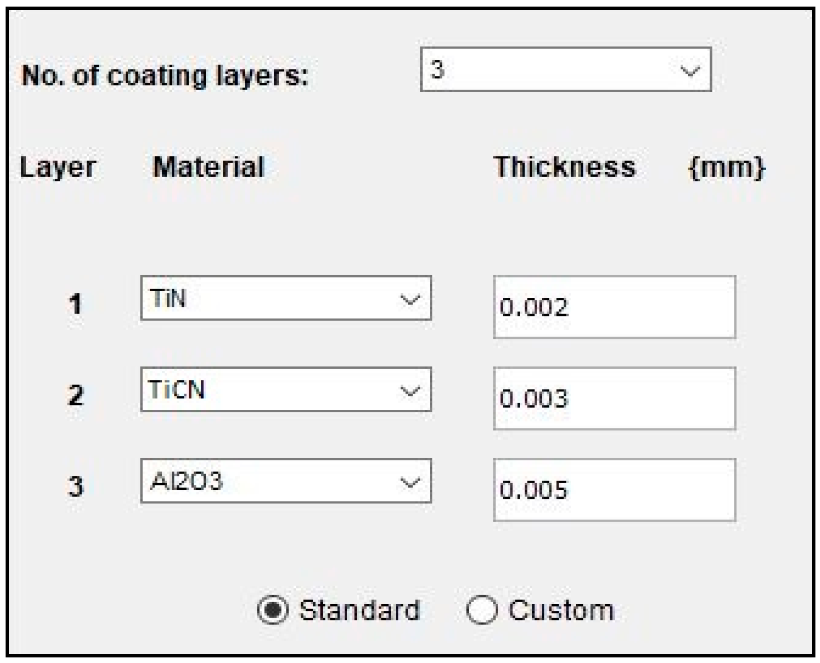
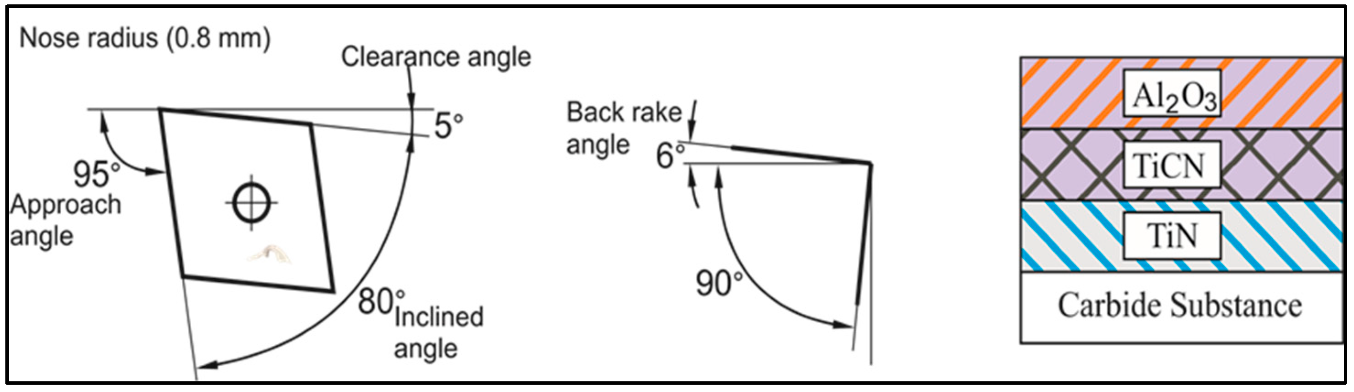
| Cutting tool | : Multilayer coated carbide insert (TiN/TiCN/Al2O3) |
| Coating layer thickness | : Al2O3: 5 µm, TiCN: 3 µm, TiN: 2 µm |
| Tool geometry | : Back rake angle −6°, negative edge inclination angle −6°, clearance angle 5°, approach angle 95°, and nose radius 0.8 mm. |
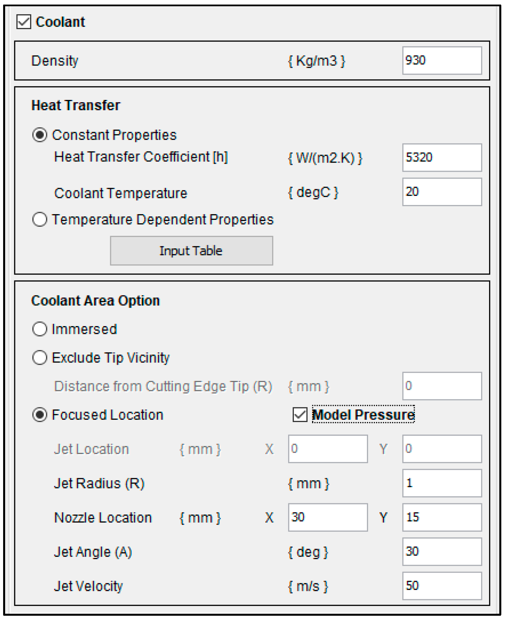
| Convective heat transfer coefficient | : 5320 W/m2·K [38]. |
| Run No. | v (m/min) | f (mm/rev) | d (mm) | Jet Angle (JA) (°) | Jet Velocity (JV) (m/s) | Nozzle Stand-off Distance (NSD) (mm) |
|---|---|---|---|---|---|---|
| 1 | 80 | 0.05 | 0.15 | 20 | 50 | 20 |
| 2 | 80 | 0.05 | 0.15 | 20 | 60 | 30 |
| 3 | 80 | 0.05 | 0.15 | 20 | 70 | 40 |
| 4 | 80 | 0.10 | 0.30 | 30 | 50 | 20 |
| 5 | 80 | 0.10 | 0.30 | 30 | 60 | 30 |
| 6 | 80 | 0.10 | 0.30 | 30 | 70 | 40 |
| 7 | 80 | 0.15 | 0.45 | 40 | 50 | 20 |
| 8 | 80 | 0.15 | 0.45 | 40 | 60 | 30 |
| 9 | 80 | 0.15 | 0.45 | 40 | 70 | 40 |
| 10 | 110 | 0.05 | 0.30 | 40 | 50 | 40 |
| 11 | 110 | 0.05 | 0.30 | 40 | 60 | 20 |
| 12 | 110 | 0.05 | 0.30 | 40 | 70 | 30 |
| 13 | 110 | 0.10 | 0.45 | 20 | 50 | 40 |
| 14 | 110 | 0.10 | 0.45 | 20 | 60 | 20 |
| 15 | 110 | 0.10 | 0.45 | 20 | 70 | 30 |
| 16 | 110 | 0.15 | 0.15 | 30 | 50 | 40 |
| 17 | 110 | 0.15 | 0.15 | 30 | 60 | 20 |
| 18 | 110 | 0.15 | 0.15 | 30 | 70 | 30 |
| 19 | 140 | 0.05 | 0.45 | 30 | 50 | 30 |
| 20 | 140 | 0.05 | 0.45 | 30 | 60 | 40 |
| 21 | 140 | 0.05 | 0.45 | 30 | 70 | 20 |
| 22 | 140 | 0.10 | 0.15 | 40 | 50 | 30 |
| 23 | 140 | 0.10 | 0.15 | 40 | 60 | 40 |
| 24 | 140 | 0.10 | 0.15 | 40 | 70 | 20 |
| 25 | 140 | 0.15 | 0.30 | 20 | 50 | 30 |
| 26 | 140 | 0.15 | 0.30 | 20 | 60 | 40 |
| 27 | 140 | 0.15 | 0.30 | 20 | 70 | 20 |
| Run. No | Fa (N) | Fc (N) | Cutting-Edge Temp. (°C) | Machined-Surface Temp. (°C) | Tool–Chip Contact Length (mm) | S/N Ratio (dB) |
|---|---|---|---|---|---|---|
| 1 | 58.913 | 101.192 | 521 | 281 | 0.15411 | −50.85 |
| 2 | 71.525 | 119.162 | 536 | 293 | 0.17124 | −51.17 |
| 3 | 97.983 | 146.312 | 565 | 304 | 0.19110 | −51.73 |
| 4 | 62.499 | 134.033 | 525 | 307 | 0.16992 | −51.33 |
| 5 | 55.395 | 158.745 | 553 | 319 | 0.19160 | −51.83 |
| 6 | 75.231 | 208.569 | 578 | 333 | 0.21440 | −52.29 |
| 7 | 87.439 | 203.531 | 551 | 362 | 0.18582 | −52.28 |
| 8 | 71.474 | 228.531 | 581 | 371 | 0.22780 | −52.74 |
| 9 | 91.346 | 253.279 | 598 | 379 | 0.25268 | −53.14 |
| 10 | 57.992 | 158.523 | 548 | 300 | 0.11258 | −51.58 |
| 11 | 65.412 | 176.226 | 581 | 311 | 0.13420 | −52.07 |
| 12 | 112.192 | 207.609 | 612 | 318 | 0.15524 | −52.57 |
| 13 | 71.761 | 184.270 | 584 | 339 | 0.13280 | −52.39 |
| 14 | 83.545 | 206.804 | 606 | 346 | 0.16760 | −52.81 |
| 15 | 108.891 | 224.507 | 638 | 353 | 0.19524 | −53.21 |
| 16 | 62.571 | 142.238 | 521 | 382 | 0.14989 | −51.35 |
| 17 | 97.679 | 178.64 | 543 | 394 | 0.16897 | −51.95 |
| 18 | 104.675 | 218.07 | 591 | 405 | 0.20897 | −52.70 |
| 19 | 69.117 | 157.718 | 601 | 331 | 0.08190 | −52.32 |
| 20 | 117.143 | 195.539 | 626 | 338 | 0.10156 | −52.80 |
| 21 | 105.564 | 216.46 | 641 | 343 | 0.12156 | −53.11 |
| 22 | 65.487 | 107.828 | 621 | 354 | 0.09192 | −52.48 |
| 23 | 76.982 | 134.382 | 643 | 363 | 0.11584 | −52.89 |
| 24 | 100.133 | 163.351 | 664 | 372 | 0.13998 | −53.31 |
| 25 | 87.426 | 131.968 | 634 | 412 | 0.10321 | −52.99 |
| 26 | 101.264 | 169.789 | 654 | 427 | 0.12016 | −53.36 |
| 27 | 113.045 | 188.296 | 682 | 439 | 0.15747 | −53.76 |
| Source | DF | Seq. SS | Contr. | Adj. MS | F-Value | p-Value |
|---|---|---|---|---|---|---|
| v | 2 | 3035.9 | 7.43% | 1517.93 | 27.33 | 0.000 |
| f | 2 | 3490.0 | 8.54% | 1744.99 | 31.42 | 0.000 |
| d | 2 | 17,630.8 | 43.13% | 8815.41 | 158.71 | 0.000 |
| JA | 2 | 1682.0 | 4.11% | 840.980 | 15.14 | 0.000 |
| JV | 2 | 14,179.3 | 34.68% | 7089.65 | 127.64 | 0.000 |
| NSD | 2 | 85.3 | 0.21% | 42.6600 | 0.770 | 0.483 |
| Error | 14 | 777.6 | 1.90% | 55.5500 | ||
| Total | 26 | 40,880.9 | 100.00% |
| Source | DF | Seq. SS | Contr. | Adj. MS | F-Value | p-Value |
|---|---|---|---|---|---|---|
| v | 2 | 33,864.2 | 61.36% | 16,932.1 | 555.87 | 0.000 |
| f | 2 | 1908.2 | 3.46% | 954.1 | 31.32 | 0.000 |
| d | 2 | 2881.6 | 5.22% | 1440.8 | 47.30 | 0.000 |
| JA | 2 | 3926.0 | 7.11% | 1963.0 | 64.44 | 0.000 |
| JV | 2 | 11,977.6 | 21.70% | 5988.8 | 196.61 | 0.000 |
| NSD | 2 | 204.7 | 0.37% | 102.3 | 3.36 | 0.064 |
| Error | 14 | 426.4 | 0.77% | 30.5 | ||
| Total | 26 | 55,188.7 | 100.00% |
| Source | DF | Seq. SS | Contr. | Adj. MS | F-Value | p-Value |
|---|---|---|---|---|---|---|
| v | 2 | 16,947.2 | 39.48% | 8473.59 | 359.16 | 0.000 |
| f | 2 | 18,149.9 | 42.29% | 9074.93 | 384.65 | 0.000 |
| d | 2 | 2015.6 | 4.70% | 1007.81 | 42.72 | 0.000 |
| JA | 2 | 2178.7 | 5.08% | 1089.37 | 46.17 | 0.000 |
| JV | 2 | 3229.0 | 7.52% | 1614.48 | 68.43 | 0.000 |
| NSD | 2 | 71.4 | 0.17% | 35.70 | 1.51 | 0.254 |
| Error | 14 | 330.3 | 0.77% | 23.59 | ||
| Total | 26 | 42,922.1 | 100.00% |
| Source | DF | Seq. SS | Contr. | Adj. MS | F-Value | p-Value |
|---|---|---|---|---|---|---|
| v | 2 | 0.029271 | 59.73% | 0.014635 | 362.91 | 0.000 |
| f | 2 | 0.006893 | 14.07% | 0.003447 | 85.46 | 0.000 |
| d | 2 | 0.000682 | 1.39% | 0.341 | 8.46 | 0.004 |
| JA | 2 | 0.000031 | 0.06% | 0.000016 | 0.39 | 0.687 |
| JV | 2 | 0.011484 | 23.43% | 0.005742 | 142.38 | 0.000 |
| NSD | 2 | 0.000079 | 0.16% | 0.000040 | 0.98 | 0.400 |
| Error | 14 | 0.000565 | 1.15% | 0.000040 | ||
| Total | 26 | 0.049005 | 100.00% |
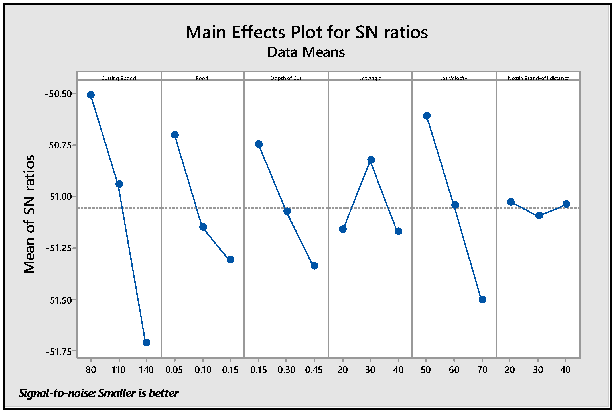
| Level | Cutting Speed (m/min) | Feed (mm/rev) | Depth of Cut (mm) | Jet Angle (°) | Jet Velocity (m/s) | Nozzle Stand-off Distance (mm) |
|---|---|---|---|---|---|---|
| 1 | −51.94 | −52.03 | −52.05 | −52.48 | −96.00 | −52.39 |
| 2 | −52.30 | −52.51 | −52.43 | −52.19 | −52.41 | −52.45 |
| 3 | −53.01 | −52.70 | −52.76 | −52.57 | −52.87 | −52.40 |
| Delta | 1.07 | 0.67 | 0.71 | 0.37 | 0.91 | 0.06 |
| Rank | 1 | 4 | 3 | 5 | 2 | 6 |
| Run No. | Experimental | Simulated | ||||||
|---|---|---|---|---|---|---|---|---|
| Fa (N) | Fc (N) | Cutting-Edge Temp. (°C) | Machined-Surface Temp. (°C) | Fa (N) | Fc (N) | Cutting-Edge Temp. (°C) | Machined-Surface Temp. (°C) | |
| 01 | 66.277 | 110.7 | 484 | 295 | 58.91 | 101.192 | 521 | 281 |
| 18 | 116.71 | 198.4 | 614 | 376 | 104.6 | 218.070 | 591 | 405 |
| 21 | 99.230 | 233.7 | 579 | 312 | 105.5 | 216.460 | 641 | 343 |
| 24 | 112.48 | 185.4 | 637 | 407 | 100.1 | 163.351 | 664 | 372 |
Disclaimer/Publisher’s Note: The statements, opinions and data contained in all publications are solely those of the individual author(s) and contributor(s) and not of MDPI and/or the editor(s). MDPI and/or the editor(s) disclaim responsibility for any injury to people or property resulting from any ideas, methods, instructions or products referred to in the content. |
© 2025 by the authors. Licensee MDPI, Basel, Switzerland. This article is an open access article distributed under the terms and conditions of the Creative Commons Attribution (CC BY) license (https://creativecommons.org/licenses/by/4.0/).
Share and Cite
Mane, S.; Patil, R.B.; Kolhe, M.L.; Roy, A.; Kamble, A.G.; Chaudhari, A. Analysis of Thermal Aspect in Hard Turning of AISI 52100 Alloy Steel Under Minimal Cutting Fluid Environment Using FEM. Appl. Mech. 2025, 6, 26. https://doi.org/10.3390/applmech6020026
Mane S, Patil RB, Kolhe ML, Roy A, Kamble AG, Chaudhari A. Analysis of Thermal Aspect in Hard Turning of AISI 52100 Alloy Steel Under Minimal Cutting Fluid Environment Using FEM. Applied Mechanics. 2025; 6(2):26. https://doi.org/10.3390/applmech6020026
Chicago/Turabian StyleMane, Sandip, Rajkumar Bhimgonda Patil, Mohan Lal Kolhe, Anindita Roy, Amol Gulabrao Kamble, and Amit Chaudhari. 2025. "Analysis of Thermal Aspect in Hard Turning of AISI 52100 Alloy Steel Under Minimal Cutting Fluid Environment Using FEM" Applied Mechanics 6, no. 2: 26. https://doi.org/10.3390/applmech6020026
APA StyleMane, S., Patil, R. B., Kolhe, M. L., Roy, A., Kamble, A. G., & Chaudhari, A. (2025). Analysis of Thermal Aspect in Hard Turning of AISI 52100 Alloy Steel Under Minimal Cutting Fluid Environment Using FEM. Applied Mechanics, 6(2), 26. https://doi.org/10.3390/applmech6020026