Optimization of Signal Detection Using Deep CNN in Ultra-Massive MIMO

Abstract

This paper addresses the evolving landscape of communication technology, emphasizing the pivotal role of 5G and the emerging 6G networks in accommodating the increasing demand for high-speed and accurate data transmission. We delve into the advancements in 5G technology, particularly the implementation of millimeter wave (mmWave) frequencies ranging from 30 to 300 GHz. These advancements are instrumental in enhancing applications requiring massive data transmission and reception, facilitated by massive MIMO (multiple input multiple output) systems. Looking towards the future, this paper forecasts the necessity for faster data transmission technologies, shifting the focus toward the development of 6G networks. These future networks are projected to employ ultra-massive MIMO systems in the terahertz band, operating within 0.1–10 THz frequency ranges. A significant part of our research is dedicated to exploring advanced signal detection techniques, helping to mitigate the impact of interference and improve accuracy in data transmission and enabling more efficient communication, even in environments with high levels of noise, and including zero forcing (ZF) and minimum mean square error (MMSE) methods, which form the cornerstone of our proposed approach. Additionally, signal detection contributes to the development of new communication technologies such as 5G and 6G, which require a high data transmission efficiency and rapid response speeds. The core contribution of this study lies in the application of deep learning to signal detection in ultra-massive MIMO systems, a critical component of 6G technology. We compare this approach with existing ELMx-based machine learning methods, focusing on algorithmic efficiency and computational performance. Our comparative analysis included the regularized extreme learning machine (RELM) and the outlier robust extreme learning machine (ORELM), juxtaposed with ZF and MMSE methods. Simulation results indicated the superiority of our convolutional neural network for signal detection (CNN-SD) over the traditional ELMx-based, ZF, and MMSE methods, particularly in terms of channel capacity and bit error rate. Furthermore, we demonstrate the computational efficiency and reduced complexity of the CNN-SD method, underscoring its suitability for future expansive MIMO systems.

1. Introduction

Wireless communication technology has continuously evolved, especially with the development of multiple input multiple output (MIMO) systems that use multiple receiving and sending antennas for data transmission. This advancement has led to the extensive study of massive MIMO systems due to the increasing demand for higher data transmission capacities, a critical component as we look ahead to 6G communication systems [1,2]. Ultra-massive MIMO has been identified as a key technology for enhancing data transmission in the 6G network [3,4,5]. Currently, 5G networks utilize various frequency bands, including sub-6GHz and millimeter wave (mmWave), catering to virtual environments and the Internet of Things (IoT). However, research and development into 6G are ongoing, aiming to support more connected devices and higher capacities, while providing faster data rates and lower latency than 5G [6]. Additionally, 6G seeks to enhance communication security and reliability and may introduce new applications, such as holographic communication. Technologies for AI and autonomous cars are also being developed in anticipation of 6G. Compared to 5G, 6G is expected to increase data rates by 10 to 100 times, supporting up to Tb/s and 10 Gb/s user experience data rates. Moreover, 6G could use flexible frequency-sharing technology, to optimize frequency reuse. Ultra-massive MIMO technology, a crucial aspect of 6G’s future, can be categorized into four main areas: frequency bands, transmission mode, intelligent transmission, and integrated network. As mentioned, 6G will support the use of terahertz frequencies ranging from 0.1 THz to 10 THz, which will aid in the development of systems and meet future needs such as the application of AI, medical devices, or autonomous driving systems that require lower latency and higher precision. This also includes high-speed internet access, allowing everyone to access increased communication resources [7,8].

In order to overcome limitations and highlight differences in wireless communications, signal detection techniques like zero forcing (ZF) and MMSE (minimum mean square error) are utilized, along with deep learning techniques [9,10]. Current 5G technology aims to provide higher data rates and lower latency than 4G, accommodating new applications like virtualization and more connected devices. Ultra-massive MIMO considers using more than 128 antenna elements at both the transmitter and receiver [11]. The Saleh–Valenzuela (SV) channel model has been selected by many researchers and is applicable in various communication formats, including hybrid beamforming, hybrid precoding, and spatial multiplexing [12]. Machine learning architecture, particularly ELMx-based systems, that includes ELM is widely used in communication for channel estimation [13],  including articles of interest regarding the application of AI in traffic prediction [14].

The main contributions of this work are summarized as follows:

• We propose the CNN-SD, which integrates three machine learning algorithms of ELM, RELM, and ORELM for signal detection. The hidden layer bias and input weight in CNN-SD are randomly generated from distributions [15,16,17].
• We foresee greater complexity with the larger number of antennas. The application of deep learning to signal detection contributes to improved performance and reduced complexity, rather than using more complex channel estimation methods.
• We developed a modeling framework for detailed learning and simultaneous regression, incorporating real and imaginary components of complex matrices into the input layers of artificial neural networks to minimize potential errors. This approach allows us to reduce the system’s overall complexity and enhance its efficiency.

The simulation results demonstrate that, in terms of mean square error (MSE), bit error rate (BER), channel capacity, outage probability, and computational time, CNN-SD performed better for signal detection.

The remainder of this paper is summarized as follows: Section 2 details the materials and methods. The proposed CNN-SD algorithm is specifically described in Section 2. Section 3 gives simulation figures to illustrate the signal detection performance of the proposed algorithm. Section 4 is the conclusions.

2. Materials and Methods

For the construction of a system model, we developed a comprehensive communication framework emphasizing ultra-massive MIMO technology, with the objective of facilitating the computation of a diverse array of results. This will be explained in Section 2.1, including massive MIMO and ultra-massive MIMO.

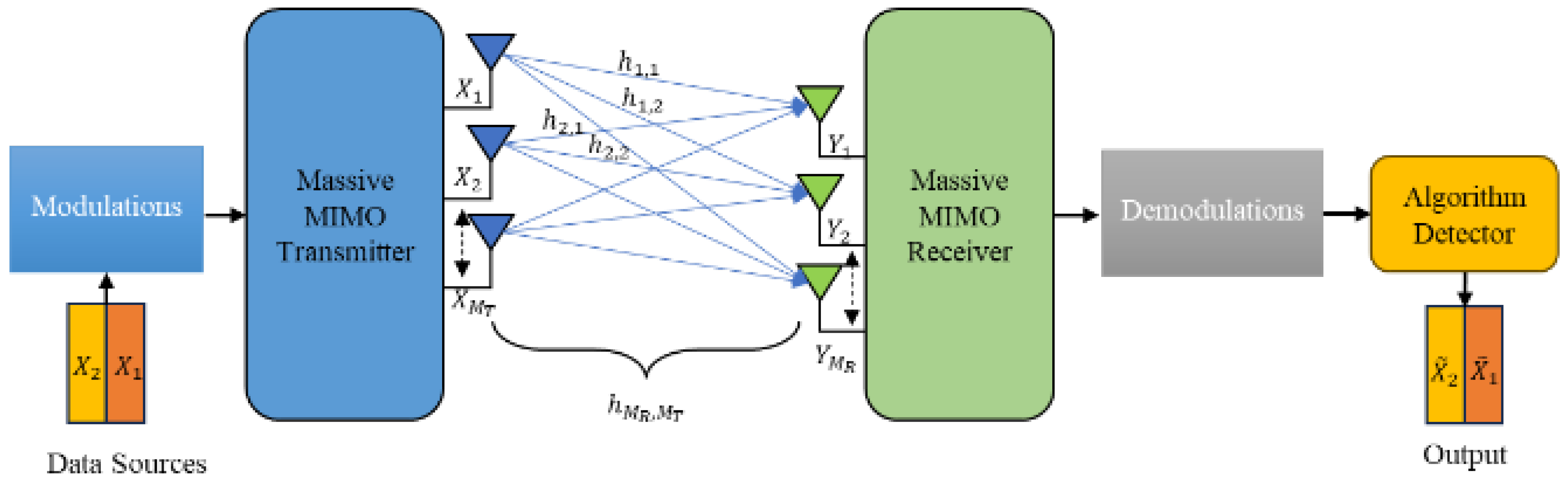
2.1. Fundamentals System Models

A simple system model has transmitting antennas ($M_T$) and receiving antennas ($M_R$). The relation between the transmitted and received signal is spatial multiplexing. The memoryless MIMO flat fading channel (narrowband model) is given by

$$Y=Hx+n$$

(1)

According to the framework of Equation (1), the matrix H, which represents a signal response channel matrix with dimensions $(M_R\times M_T)$, is utilized to clarify the application of both massive MIMO and ultra-massive MIMO systems. Furthermore, the variable n, defined as an additive white complex Gaussian noise vector with dimensions $(M_R\times 1)$, is recognized as a primary noise model in information theory. This model is specifically crafted to replicate the effects of the diverse random processes commonly observed in natural settings. The matrix representation thus effectively captures the relationship between transmitted and received signals, illustrating the intricate dynamics of signal propagation in these advanced communication systems as

$$\left[\begin{array}{c}{Y}_1\\ Y_2\\ ⋮\\ Y_{M_R}\end{array}\right]=\left[\begin{array}{cccc}{h}_{11}& h_{12}& \cdots & h_{1,M_T}\\ h_{12}& h_{22}& \cdots & h_{2,M_T}\\ ⋮& ⋮& \ddots & ⋮\\ h_{M_R,1}& h_{M_R,2}& \cdots & h_{M_R,M_T}\end{array}\right]\left[\begin{array}{c}{X}_1\\ X_2\\ ⋮\\ X_{M_T}\end{array}\right]+\left[\begin{array}{c}{n}_1\\ n_2\\ ⋮\\ n_{M_R}\end{array}\right]$$

(2)

2.1.1. Massive MIMO

Massive MIMO has been much researched regarding channel response. First, as illustrated in Figure 1, we investigate a typical massive MIMO system. A block diagram is assumed for delivering data sources from the X (vector of transmitted signals) to the Y (vector of received signals). In this model, the channel parameter h represents the communication link between nodes X and Y, which clearly shows the behavior of Equation (1). Rayleigh channels are commonly used in massive MIMO systems, due to their ease and accuracy in simulating the internal conditions of the communication channel. They can also estimate the impact of low-risk distribution in a large number of wireless communications. However, it should be noted that using Rayleigh channels in massive MIMO often results in simulating channel states invariantly. Since the simulation is local, this approach may yield results that are not entirely accurate to natural conditions.Including the future possibilities of 6G, studies across various works have found that the current number of antennas in massive MIMO still face operational limitations in the THz frequency bands, starting with as few as 16 antennas. Meanwhile, the concept of ultra-massive MIMO, discussed in this research, explores the use of a significantly larger number of antennas, up to 256, representing a full-capacity model. Further details will be provided in the subsequent section.

2.1.2. Ultra-Massive MIMO

This paper focuses on different channels based on potential real situations. This was considered as much as possible by using the Saleh–Valenzuela signal model, in which the signal consists of a combination of discrete radiation bundles. This is a typical model for mmWave signals, which have high reflectivity and low diffusion. Mathematically, the ray/cluster signal matrix can be represented as

$$H=\sum _{v=1}^{Nclust}\sum _{u=1}^{Nray}{\beta }_{u,v}{a}_{rx}\left(Ao{A}_{u,v}\right)a_{tx}{\left(Ao{D}_{u,v}\right)}^{\ast }$$

(3)

where u and v denote the number of subarrays at $M_T$ and $M_R$, and where the signal comprises cluster $N_{clust}$ is the cluster angle. In each group, $N_{rays}$ is the ray, where each ray is considered in the loop of the simulation, accounting for the multipath effects encountered by the signal. Cluster ${\beta }_{u,v}$ shows complex gain. In addition, $Ao{D}_{u,v}$ is the angle of departure (from the transmitting array) and $Ao{A}_{u,v}$ is the angle of arrival (from the receiver array). The subsequent sending and receiving arrays are $a_{tx}\left(Ao{D}_{u,v}\right)$ and $a_{rx}\left(Ao{A}_{u,v}\right)$, respectively.

This section focuses on signal detection in ultra-massive MIMO systems, which is crucial for transmitting large amounts of data across multiple transmitting antennas arranged in a matrix, while simultaneously dealing with interference signals. k-QAM modulation is commonly employed to introduce and simulate intricate scenarios in ultra-massive MIMO systems, specifically in relation to the proposed modulation schemes for 6G. The modulation process is controlled by the phase of constellation mapping. The procedure involves receiving binary bits as input, converting them into complex numbers, and subsequently using them as symbols. The analysis involves a multiple-input multiple-output (MIMO) wireless system that experiences flat fading. This system utilizes multiple transmitting antennas $M_T$ and multiple receiving antennas $M_R$. The symbol $X_N\left(p\right)$ denotes the transmission conducted by the antenna $M_T$ at a precise moment p. The symbols that have been sent are organized into a vector of length $M_T$ such as $X_N\left(p\right)={[X_1\left(p\right),\dots ,X_{M_T}\left(p\right)]}^T$, which is referred to as

$$X_N\left(p\right)=\left|N\left(p\right)\right|cos(arg\left\{N\left(p\right)\right\})cos\left(2\pi f_{c}p\right)-\left|N\left(p\right)\right|sin(arg\left\{N\left(p\right)\right\})sin\left(2\pi f_{c}p\right)$$

(4)

k is the number of modulations that covers all QAM modulation,

where $\left|u\right(t\left)\right|$ and $argu\left(t\right)$ are the amplitude and phase of the complex baseband signal, respectively.

2.2. Traditional Method

This paper focuses on the critical role of specific technology or methods in enhancing a multiple-input multiple-output (MIMO) system in Figure 2. By leveraging this technology, we aim to augment the system’s capacity, primarily by improving performance metrics such as the bit error rate. Our study involves a comprehensive comparison between conventional signal detection techniques, including ZF and MMSE, and advanced methods based on the ELMx algorithm, namely ELM, RELM, and ORELM. Moreover, we introduce the convolutional neural network-based signal detection CNN-SD algorithm, proposing it as a novel approach for further performance enhancement in MIMO systems.

2.2.1. Zero Forcing Detector

Zero forcing was an early concept in channel estimation. By detecting signals, this type of estimation is classified as a one-dimensional (1D) estimator, which means that the channel estimation is performed using test cycles. In one dimension, whether frequency or time, (ZF) signal detection reduces the amount of squared error between the received signal and the estimated value. As a result, it is possible to find ${\tilde{X}}_{ZF}$ signal detection by

$${\widehat{H}}_{ZF}={\mathrm{argmin}}_{H_{ZF}}{∥Y-H_{ZF}X|∥}^2$$

(5)

On the other hand, the signal detection can be written in the following form:

$$\tilde{X}=H^{†}Y$$

(6)

All transmitting and receiving antennas, the impulse response signals are encapsulated and presented in the form of a matrix by

$${\tilde{X}}_{ZF}=Y{H}^H{\left(H{H}^H\right)}^{-1}$$

(7)

In this formulation, ${(\ast )}^H$ is designated as the conjugate transpose of the matrix, and ${(\ast )}^{-1}$ pertains to the inverse of the matrix.

2.2.2. MMSE Signal Detector

The MMSE signal detector is an algorithms referenced in many works. It is calculated similarly to channel estimation [18,19]. It is the second comparator that we used for signal estimation, because it is the most commonly used and most complex calculation method. As a result, it is more accurate than the ZF signal detection given by

$${\tilde{X}}_{MMSE}=\mathrm{argmin}{∥Y-{\tilde{X}}_{MMSE}H∥}^2$$

(8)

The detection strategy includes accounting for noise during the computation process, which is measured by

$${\tilde{X}}_{MMSE}=Y{H}^H{(H{H}^H+\frac{{{\sigma }_n}^2}{{{\sigma }_h}^2}I)}^{-1}$$

(9)

In this context, $\mathbf{I}$ denotes the identity matrix of size $M_T\times M_R$, while ${{\sigma }_n}^2$ represents the noise variance, which is inversely proportional to the signal-to-noise ratio (SNR). Additionally, all signal response energies have been normalized, as exemplified by

$$E\left\{{\left|h_{M_R,M_T}\right|}^2\right\}={{\sigma }_h}^2$$

(10)

2.3. Machine Learning Method

2.3.1. Extreme Learning Machine (ELM)

This study introduces an accelerated learning method for single hidden layer feedforward networks (SLFNs) [20,21], which is designed to effectively manage networks with $\tilde{N}$ hidden neuron nodes. Additionally, the method is tailored to handle $\tilde{N}\le$N training samples. The focus is on significantly speeding up the learning process in SLFNs, thereby enhancing training efficiency and effectiveness. Extreme learning machine (ELM), an algorithm within the machine learning domain that employs neural networks, is known for its impressive efficiency in regression tasks and an accelerated learning rate. This was substantiated through both theoretical analysis and empirical validation. The architectural framework of ELM is detailed in Figure 3, providing a clear visual representation of its structure. n and m respectively denote the numbers of input and output data. The analysis utilizes the ELM training process with N training samples $\left(X_i,t_i\right)$, where $X_i={[X_{i1},X_{i2},\dots ,X_{in}]}^T$ represents the input data, and $t_i={[t_{i1},t_{i2},\dots ,t_{im}]}^T$ the output data. The approach to detecting patterns in SLFNs employs a mathematical model, outlined as follows:

$${\widehat{t}}_j={\sum _{i=1}^{\tilde{N}}\beta }_{i}o\left(c_i·X_j+V_i\right),j=1,2,\dots ,N$$

(11)

$c_i={[c_{i1},c_{i2},\dots ,c_{in}]}^T$ is the input weight vector that connects to the i-th hidden neuron, and $\beta ={[{\beta }_{i1},{\beta }_{i2},\dots ,{\beta }_{im}]}^T$ refers to the output weight vector of the i-th hidden neuron node. The term $V_i$ is the bias of the i-th hidden neuron node, and $c_i$ indicates the activation function in SLFNs. Unlike other machine learning algorithms, ELM can randomly assign the input weight $c_i$ and bias $V_i$. A significant feature of ELM, contributing to its regression performance, is its verification of zero error, which allows an accurate approximation of all $\mathbf{N}$ samples as $i=1Ntj-tj=0$; i.e., the $\mathbf{N}$ equations can thus be compactly expressed as

$$H\beta =T,where\beta ={\left[\begin{array}{c}{\beta }_1\\ ⋮\\ {\beta }_{\tilde{N}}\end{array}\right]}_{\tilde{N}\times m}^T,T={\left[\begin{array}{c}{T}_1\\ ⋮\\ T_N\end{array}\right]}_{N\times m}^T$$

(12)

$$H(c_i,\cdots ,c_N,V_i,\cdots ,V_N,X_i,\cdots ,X_N)={\left[\begin{array}{ccc}o(c_1·X_1+V_1)& \cdots & o(c_{\tilde{N}}·X_1+V_{\tilde{N}})\\ ⋮& \cdots & ⋮\\ o(c_1·X_N+V_1)& \cdots & o(c_{\tilde{N}}·X_N+V_{\tilde{N}})\end{array}\right]}_{N\times \tilde{N}}$$

(13)

where H is the neural network’s hidden layer output matrix and T is the training data target matrix. The variable H represents the output matrix of the hidden layer in the neural network, whereas T represents the matrix that contains the training data targets. Moreover, $\widehat{\beta }$ was identified as the solution with the minimum magnitude in the least-squares approach, which is essential to the linear system of the ELM solution.

$$\widehat{\beta }=H^{P}T$$

(14)

where ${(\ast )}^P$ is the Moore–Penrose pseudoinverse.

2.3.2. Regularized Extreme Learning Machine (RELM)

While the ELM has proven effective in numerous applications, the implementation of the $\tilde{N}$ method is recommended to circumvent overfitting and underfitting. As the study in [22] suggests, smaller norm parameters in the RELM designed for SLFNs with a sigmoid function can lead to improved generalization. This equation is versatile and applicable to various activation functions and hidden neuron nodes like kernels, specifically to resolve challenges in the $l_2$ norm of $\beta$. Consequently, RELM can be described as a method by which

$$\begin{array}{c}\mathrm{minimize}\\ \left({\beta }_0,\beta \right){\in }^{\tilde{N}x1}\end{array}\frac{C}{2}{∥H\beta +{\beta }_0-t∥}_2^2+\frac{(1-a)}{2}{∥\beta ∥}_2^2+a{∥\beta ∥}_1$$

(15)

When just the $l_2$ norm penalty $(\alpha =0)$ with ${\beta }_0=0$ is considered, the RELM formula is given where C and ${\beta }_0$ are regularization parameters.

$$\widehat{\beta }={(H^{H}H+\frac{I}{C})}^{-1}{H}^{H}t$$

(16)

2.3.3. Outlier-Robust Extreme Learning Machine (ORELM)

Recent modifications to the ORELM aimed to enhance its proficiency in the $l_1$ norm for outlier-producing techniques. Such advancements can be realized through the application of the ELM [23], as elaborated by

$$\widehat{\beta }=\begin{array}{c}\mathrm{argmin}\\ \beta \end{array}{∥\tau H\beta -t∥}_1$$

(17)

The optimal solution to the outlined optimization problem is obtained utilizing the standard $l_2$ norm.

$$\widehat{\beta }=\begin{array}{c}\mathrm{argmin}\\ \beta \end{array}{∥\tau H\beta -t∥}_1+\frac{1}{2C}{∥\beta ∥}_2^2$$

(18)

The specific processes of the ELMx-based algorithm are summarized in Algorithm 1. Noting, the ELMx based algorithm is used to obtain the estimated channel matrix in Algorithm 1.

Algorithm 1 ELM, RELM and ORELM algorithm.

1: Input: Real and Imaginary number $X\in {\mathbb{R}}^{n\times l}$, $Y\in {\mathbb{R}}^{n\times l}$ 2: Output: $\tilde{\mathbf{X}}$. 3: Initialization: Randomly assign input weight $c_i$ and bias $V_i$ for each hidden neuron i, where $i=1,2,\dots ,L$. 4: Hidden Layer Output Matrix Calculation: 5: for $i=1$ to N do 6:     Calculate the hidden layer output vector $t_i$ for each input $X_i$ using the activation function $o\left(x\right)$: 7:     $t_i=o(c_i·x_i+V_i)$ 8: end for 9: Form the hidden layer output matrix H using all $H_i$. 10: Output using Equations (14), (16) and (18).

2.4. Proposed Method

Architecture of The Proposed Convolutional Neural Network for Signal Detection (CNN-SD)

A model of a serial data processing system known as a convolutional neural network (CNN) was developed to recognize and manipulate widely connected data. The basic equation is as follows:

$$O\left(t\right)=\sum _{z=0}^{L-1}I\left(z\right)·w(t-z)+b$$

(19)

$O\left(t\right)$ represents the output of the 1D convolution at position t on the output signal O, $I\left(z\right)$ denotes the value of the input data signal I at position z., $w(t-z)$ corresponds to the value of the filter w at position $(t-z)$, and b is the bias term added to the result after the convolution operation if bias is used. L is the length of the input signal I and the length of the filter w, which is also the size of the filter. This equation shows how to perform 1D Convolution using the input signal I and filter, and including the bias term b if given. To obtain $O\left(t\right)$ in the output signal I, which multiplies and adds values from all positions in I, we use the filter w, shifted by I positions on I. To process the fully connected layer, it receives data from the previous layer as a vector of variable values or feature values. The importance of each feature can be adjusted by multiplying it by a weight and adding a bias value to allow the system to learn how the data looks and create connections between features. The linear layer

$$y=Wx+b$$

(20)

y is the output vector of the linear layer with dimensions $(m,1)$, where m is the number of output layers we need. W is a weight matrix with dimensions $(m,n)$ and is used to multiply the input x. x is an input data vector with dimensions $(n,1)$, where n is the number of data features. b is a bias vector with dimension $(m,1)$ and is added to the result after multiplication by W. The rectified linear unit (ReLU) is a mathematical function commonly used in neural networks and deep learning as an activation function to process data within a layer. The results obtained by multiplying the feature values by weights and adding bias values are sent to an activation function to generate the output values of this layer. The ReLU activation function sets each layer value to zero if it is less than zero and retains the same value if it is greater than or equal to zero. The ReLU enables neural networks to learn effectively and accelerates their computations. The functional representation of the neural network ReLU function is as follows:

$$f\left(x\right)=max(0,x)$$

(21)

where if the value x is positive or equal to 0, then the value $f\left(x\right)$ will be x itself. If the value of x is less than 0, then $f\left(x\right)$ will be zero. In the initial phase of data preparation, the role of information is critical. This phase is methodically divided into two primary categories, as delineated in Figure 4. The first category, designated as ‘training data’, consists of variably prepared data from ultra-massive MIMO systems, intended to facilitate the algorithm’s capabilities in computation and memory retention. The second category, named ‘teaching data’, is structured to enable the algorithm to assimilate and accurately reproduce the desired outputs. The differentiation between these data types is established based on their channel response attributes within the ultra-massive MIMO communication system after the data preparation stage. The sequential procedures of the CNN-SD algorithms are comprehensively outlined in Algorithm 2, providing a clear framework for the algorithmic workflow.

Algorithm 2 CNN-SD algorithm.

1: Input: Real and Imaginary number $X\in {\mathbb{R}}^{n\times l}$, $Y\in {\mathbb{R}}^{n\times l}$ 2: Output: $\tilde{\mathbf{X}}$. 3: Initialization: Randomly assign input weight $W_i$ and bias $b_i$ for each hidden neuron i, where $i=1,2,\dots ,L$. 4: procedure Processing(X) 5:       $X_{conv1}\leftarrow \mathrm{ReLU}({\mathbf{W}}_{conv1}\ast X+b_{conv1})$ 6:       $X_{conv2}\leftarrow \mathrm{ReLU}({\mathbf{W}}_{conv2}\ast X_{conv1}+b_{conv2})$ 7:       $X_{flat}\leftarrow \mathrm{Flatten}\left(X_{conv2}\right)$ 8:       $X_{fc1}\leftarrow \mathrm{ReLU}({\mathbf{W}}_{fc1}·X_{flat}+b_{fc1})$ 9:       $X_{fc2}\leftarrow \mathrm{ReLU}({\mathbf{W}}_{fc2}·X_{fc1}+b_{fc2})$ 10:     $X_{fc3}\leftarrow \mathrm{ReLU}({\mathbf{W}}_{fc3}·X_{fc2}+b_{fc3})$ 11:     $\widehat{X}\leftarrow {\mathbf{W}}_{predict}·X_{fc3}+b_{predict}$ 12:     return $\widehat{X}$ 13: end procedure

2.5. Channel Capacity

The concept of the Shannon capacity of a channel is centered on the maximum data rate that can be reached within a certain bandwidth (BW) and at a specific signal-to-noise ratio. This theoretical capacity suggests a decrease in bit error rate (BER) that is challenging to achieve in real-world scenarios. However, as link level design techniques evolve, the actual data rate for noise channels is approaching this theoretical boundary, as discussed in [24]. Often measured in bits per second (bps)/Hz or equivalent units, a high channel capacity denotes the communication system’s capability for swift and effective data transmission. It is formulated as

$$C={log}_{2}det\left[I_{M_R}+\frac{P_t}{P_n{M}_T}H{H}^H\right]$$

(22)

Here, $I_{M_R}$ is the identity matrix with dimensions ($M_R\times M_R$), H characterizes the channel response sized size ($M_T\times M_R$), ${(\ast )}^H$ is the conjugate transpose, and $P_t/P_n$ quantifies the signal noise ratio (SNR). In estimating the capacity of the channel, our examination included channel responses obtained through the LS method, the prevalent MMSE method, and three additional approaches rooted in machine learning applications, namely ELM, RELM, and ORELM. The formula for calculating the estimated capacity within the CNN-SD model is prescribed as follows (6) to produce (23).

2.6. Outage Probability

Another primary performance indicator in communication techniques is the outage probability, as discussed in [20]. This is often expressed as a percentage and depends on the channel’s state and the interference in the system. Outage probability measures the risk that a communication signal may not be received or may be lost. If the outage probability is low, the communication system is efficient in transmitting data. The outage probability can be determined as follows:

$$P_{out}(C_{es}<R)$$

(23)

where R is the rate of capacity. As a consequence, the most favorable course of action for the transmitter is to employ data encryption. This decision is contingent upon the channel gain being sufficient to accommodate the desired rate denoted as R. Under such circumstances, the attainment of dependable communication becomes feasible; otherwise, an outage is incurred. In the presence of a fading gain represented as h, one may conceive of the channel as permitting the flow of information. Provided that the volume of data surpasses the designated rate, the prospect of reliable decoding becomes attainable. The Saleh channel’s outage probability, as a function of the transmission rate R, can be expressed as follows:

$$P_{out}\left(R\right)=1-exp\left(\frac{-2^R-1}{SNR}\right)$$

(24)

$P_{out}$ signifies the outage probability of the system, characterized by how the destination performs detection when relying only on the received signals from the relay node.

2.7. Total Loss of Algorithm

2.7.1. Mean Square Error (MSE)

The efficacy of machine learning algorithms can be analyzed through multiple approaches. Consequently, mean squared error (MSE) was chosen for the performance analysis, to yield definitive conclusions, as corroborated by references [11,12]. This metric, frequently used in performance evaluation, requires calculating the error $\tilde{X}$, which represents the difference from the actual X, and then averaging this error. Based on this difference, the gradient of loss is computed and utilized for backpropagating the weights. The next step involves applying gradient descent in the subsequent training phase to lower losses. The loss function used in regression is presented by

$$MS{E}_N=\frac{1}{N}{\sum _{i=1}^N\left(X-{\tilde{X}}_i\right)}^2$$

(25)

2.7.2. Training Loss

The total loss can help us check the feasibility of the dataset between trainings, because it can specify the range to test to obtain an appropriate dataset. Practically, the mean loss is calculated for each batch and then averaged across all the batches within an epoch. This provides a comprehensive assessment of the model’s performance on the training data, helping to follow its progress over time. Considering the fast-processing time, calculating the total number of training rounds in epochs is performed as follows:

$$T_B=T_D/B_S$$

(26)

where $T_B$ is the total number of batches, $T_D$ is total data size, and $B_S$ is the batch size. For determination of the number of samples that will be distributed across the network, the batch size is essential. When training a deep learning model, the average loss is typically computed over the entire training dataset, in small batches of samples. This is known as batch training. This is because training the model on the entire dataset in one go could be computationally expensive, and it could also cause the model to overfit on the training data.

2.7.3. Validation Loss

The formula for calculating validation loss is likely MSE (25) but we only considered the amount of validation data to calculate, where M is the number of an epochs and f is the loss function. However, we calculated the validation loss as

$$V=\frac{1}{M}\sum f(\widehat{Y_d},Y_d)$$

(27)

where $\widehat{Y_d}$ is prediction data and $Y_d$ is teaching data. In addition, the interpretation of the results was very important and was divided into three parts: Underfitting refers to a situation in scenario 1 where the results indicate that additional training is required to decrease the loss experienced during the training process. Alternatively, we can enhance the training data by either acquiring additional samples or augmenting the existing data. Overfitting occurs when, in scenario 2, the validation loss surpasses the training loss. In scenario 3, a good fit is characterized by the training loss and validation loss decreasing and reaching a stable point.

3. Result and Discussion

3.1. Dataset Setup

The dataset employed consisted of three components: training data, testing data, and validation data. These components encompassed two datasets: the received signal data set, denoted as Y, and the transmitted data set, denoted as X, in accordance with the principles of communication systems. We collected and simulated a total of 100,000 datasets.

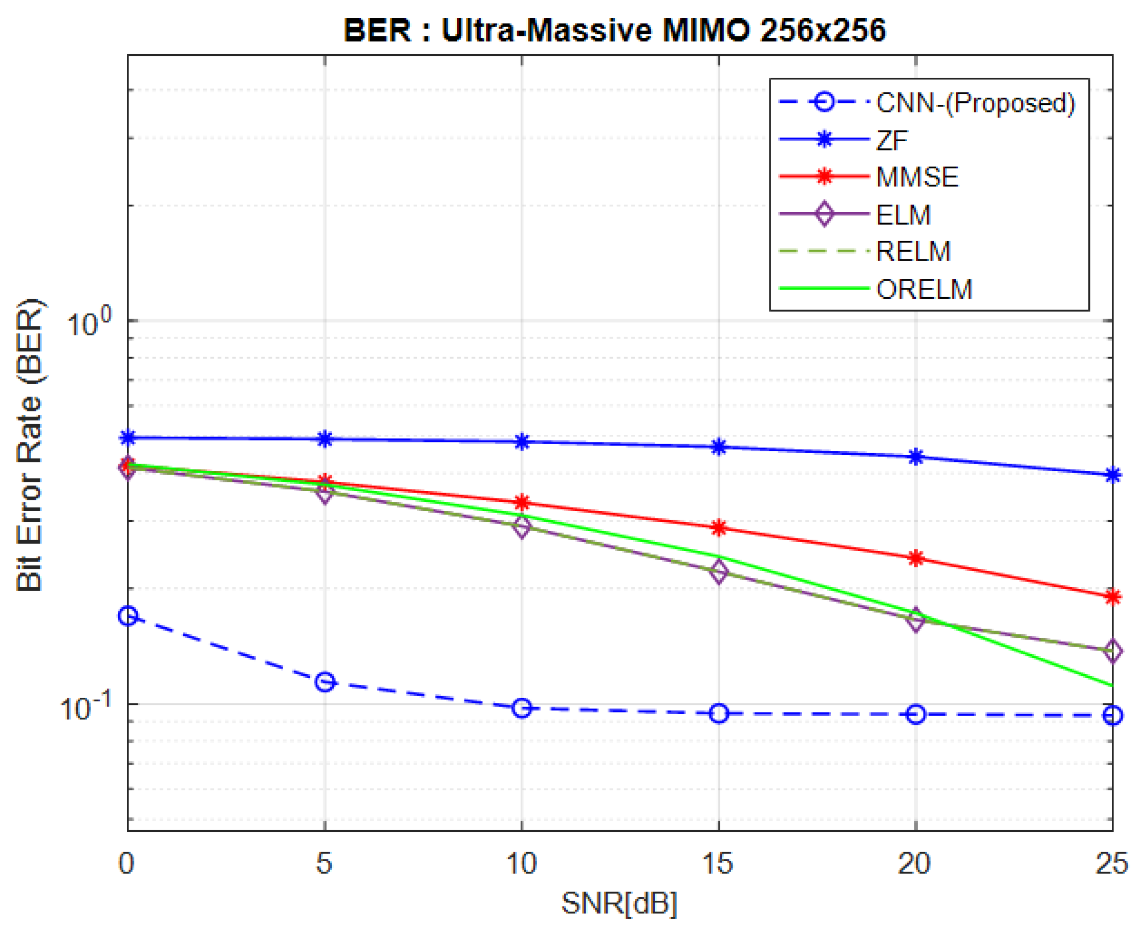
3.2. MSE and BER

This section of the study focuses on evaluating the mean square error (MSE) and bit error rate (BER), as well as assessing the effectiveness of zero forcing (ZF), minimum mean square error (MMSE), and ELMx-based signal detection approaches in confirming the performance of several CNN-SD algorithms. These strategies were evaluated in ultra-massive MIMO systems that included 256 transmitting and receiving antennas, each with 256QAM modulation mapping and a certain number of pilots. The attributes and approaches of the ELMx-based and CNN-SD algorithms are explained in Algorithms 1 and 2, correspondingly. The results of the comparative mean squared error (MSE) performance are shown in Figure 5. It was noted that ZF, because of its more rudimentary approach, was less successful compared to the other four methodologies. On the other hand, MMSE outperformed the least squares (LS) method, because of its increased complexity. The ELMx-based methodology, a machine learning technique, outperformed both ZF and MMSE by effectively using large training and testing datasets to accurately replicate the necessary data. The CNN-SD approach distinguished itself by showing a superior performance, which was attributed to its unique structural arrangement, which is optimized for exceptional results.

Figure 6 shows the performance of BER for all signal detection techniques in an ultra-massive MIMO-based communication system, which included 256 transmitting antennas (MT) and 256 receiving antennas (MR). The CNN-SD outperformed the fundamental approaches such as LS, MMSE, and ELMx-based machine learning in signal detection. The results revealed that the BER performance of the CNN-SD algorithm was the best among all methods.

3.3. Model Validation

Figure 7 shows the performance of the good fit learning curve for training loss and validation loss, and it shows that the values were closely grouped around the range of 1–3%. Therefore, the model exhibited a strong aptitude for learning. This model can be utilized to make precise predictions for previously unseen data. Alternatively, it can be referred to as a model that exhibits the ability to apply its knowledge to unfamiliar data. We divided the 100,000 datasets into 60% training data, 20% testing data, and 20% validation data, for our proposed method.

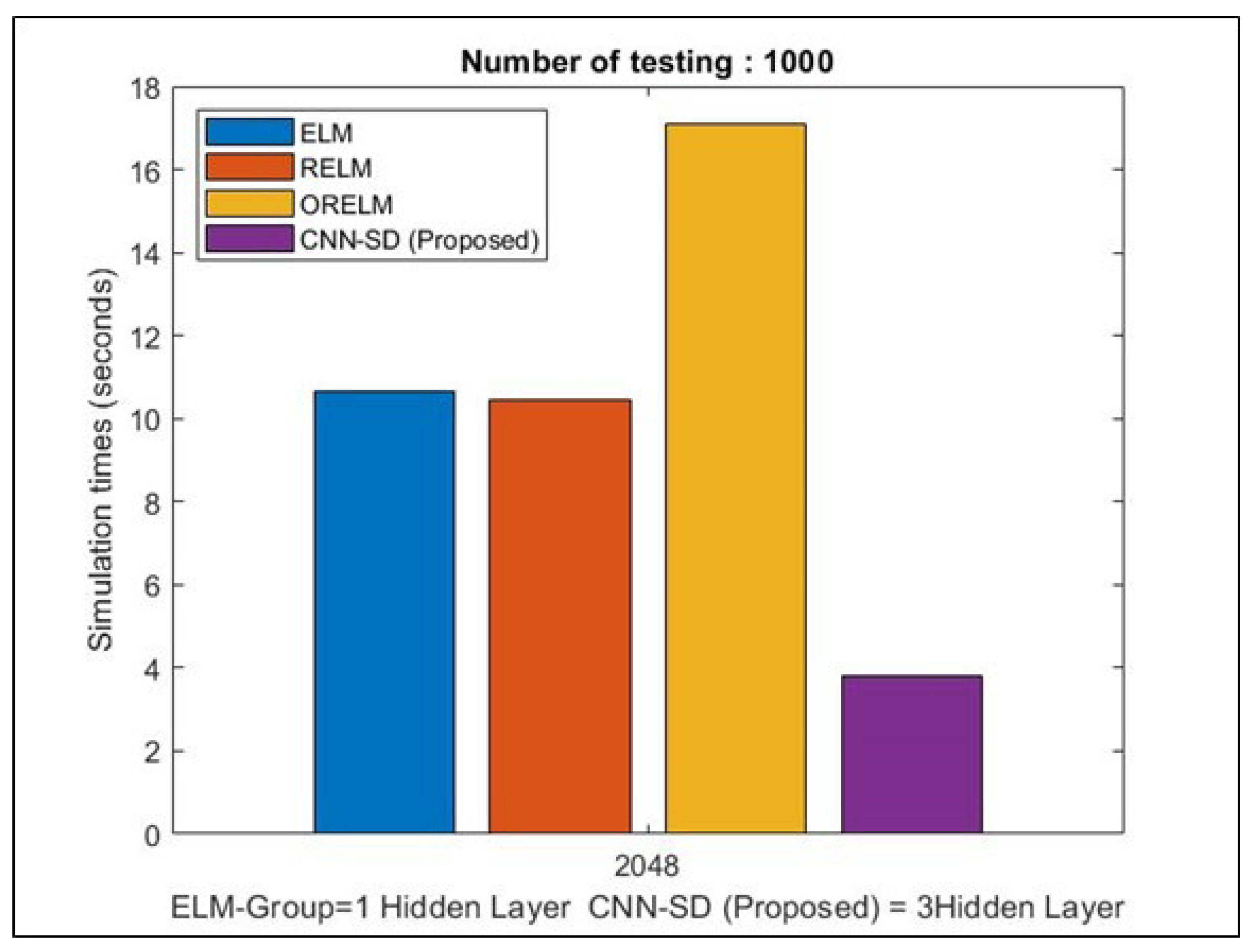
3.4. Computational Time

Figure 8 shows that the computation time was different in the computational comparison between ELMx and CNN-SD, according to the computational complexity for the number of nodes from 2048 nodes. The result for ELMx, such as ELM RELM and ORELM, revealed that the computational time was higher than CNN-SD because the data management in CNN-SD had a batch size that could help reduce the use of computer resources. This is because training on a large dataset can reduce communication time between processors. It can significantly help reduce the use of computer resources and the management of data in RAM. This is important when training models that are data-intensive or that have complex structures.

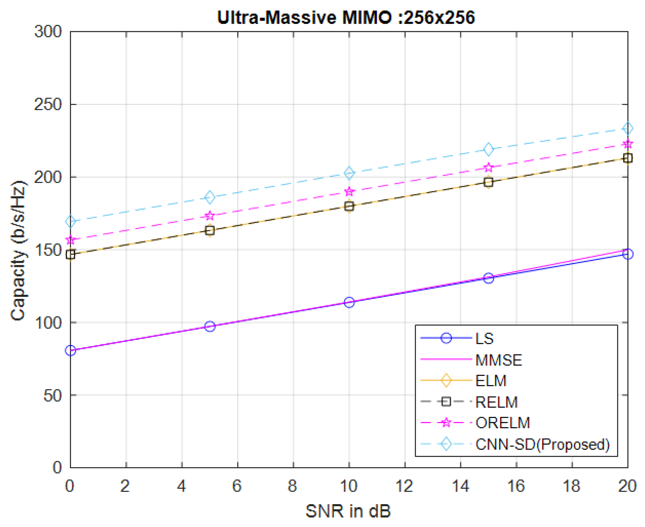
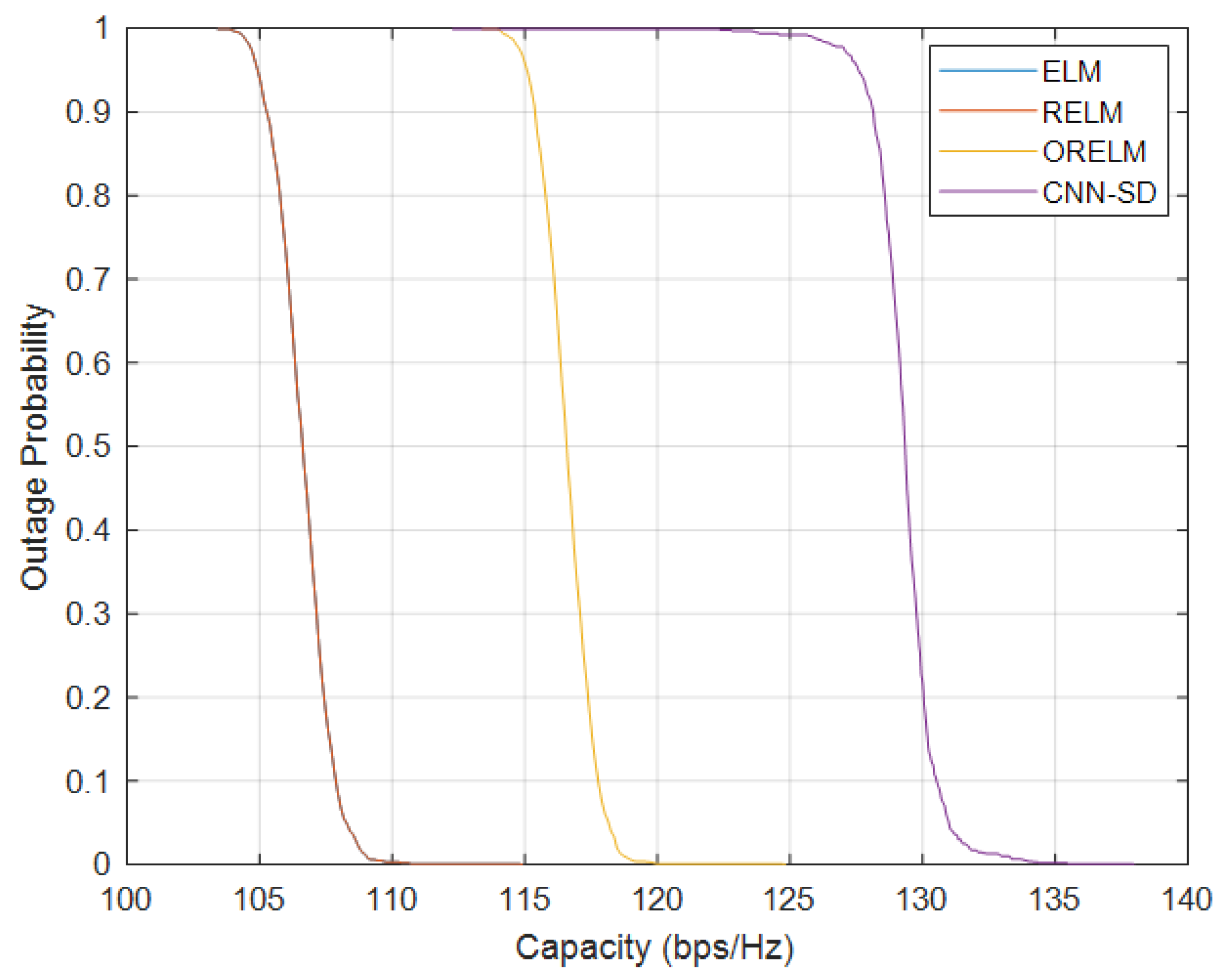
3.5. Channel Capacity and Outage Probability

Another focus of this section was on the performance metrics of channel capacity and outage probability within ultra-massive MIMO systems. Equation (19) was used for processing and comparing the channel capacity, as presented in Figure 9 and Figure 10.

Meanwhile, for determining the outage probability, Equations (20) and (21) were utilized, as demonstrated in Figure 10. The test result for channel capacity vs. SNR shows that the machine learning algorithm ELM, RELM, and ORELM techniques provided a lower channel capacity than the CNN-SD techniques. In Figure 9, the CNN-SD at 10 SNRdB had a capacity 200 bps/Hz more than the ELMx-based techniques. It is apparent that the ultra-massive MIMO channel is highly likely to achieve high capacity. At a 90% probability level, the capacities stand at 105 bps/Hz for ELM, 105 bps/Hz for RELM, and 116 bps/Hz for ORELM. Consequently, this demonstrates a significant likelihood of high channel capacity when compared to ELM, RELM, and ORELM. The CNN-SD, with a capacity of 128 bps/Hz, exhibited excellent performance in line with the method, as depicted in Figure 10.

4. Conclusions

Ultra-massive MIMO systems, representing a significant future advancement, incorporate additional communication antennas and new techniques or procedures that can enhance system efficiency and problem-solving capabilities. This paper focused on finding methods that lead to more effective communication and reduce issues. One such approach was the introduction of a CNN-SD deep learning signal detection technique within an ultra-massive MIMO system. The authors employed various techniques for comparison with the LS, MMSE, and ELMx-based machine learning groups. Three algorithms of ELM, RELM, and ORELM, along with the proposed CNN-SD, were examined to assess their performance for signal detection. The analysis of MSE, BER, capacity, and outage probability demonstrated that CNN-SD outperformed the other algorithms. Therefore, for future systems utilizing ultra-massive MIMO, CNN-SD emerges as the optimal choice for signal detection. In our future work, we aim to enhance the efficacy of our proposed method by employing a strategy that integrates score combination techniques and multi-scale neural networks, as well as exploring additional neural network architectures for performance optimization.

References

- Huo, Y.; Lin, X.; Di, B.; Zhang, H.; Hernando, F.J.L.; Tan, A.S.; Mumtaz, S.; Demir, Ö.T.; Chen-Hu, K. Technology Trends for Massive MIMO towards 6G. arXiv 2023, arXiv:2301.01703. [Google Scholar]
- Wang, X.; Kong, L.; Kong, F.; Qiu, F.; Xia, M.; Arnon, S.; Chen, G. Millimeter wave communication: A comprehensive survey. IEEE Commun. Surv. Tutor. 2018, 20, 1616–1653. [Google Scholar] [CrossRef]
- Zheng, Y.; Wang, C.X.; Yang, R.; Yu, L.; Lai, F.; Huang, J.; Feng, R.; Wang, C.; Li, C.; Zhong, Z. Ultra-massive MIMO channel measurements at 5.3 GHz and a general 6G channel model. IEEE Trans. Veh. Technol. 2022, 72, 20–34. [Google Scholar] [CrossRef]
- Dilli, R.; Chandra, R.; Jordhana, D. Ultra-Massive MIMO Technologies for 6G Wireless Networks. Eng. Sci. 2021, 16, 308–318. [Google Scholar] [CrossRef]
- Wang, C.X.; Wang, J.; Hu, S.; Jiang, Z.H.; Tao, J.; Yan, F. Key Technologies in 6G Terahertz Wireless Communication Systems: A Survey. IEEE Veh. Technol. Mag. 2021, 16, 27–37. [Google Scholar] [CrossRef]
- Faisal, A.; Sarieddeen, H.; Dahrouj, H.; Al-Naffouri, T.Y.; Alouini, M.S. Ultramassive MIMO Systems at Terahertz Bands: Prospects and Challenges. IEEE Veh. Technol. Mag. 2020, 15, 33–42. [Google Scholar] [CrossRef]
- Murshed, R.U.; Ashraf, Z.B.; Hridhon, A.H.; Munasinghe, K.; Jamalipour, A.; Hossain, M.F. A CNN-LSTM-based Fusion Separation Deep Neural Network for 6G Ultra-Massive MIMO Hybrid Beamforming. IEEE Access 2023, 11, 38614–38630. [Google Scholar] [CrossRef]
- Sarieddeen, H.; Alouini, M.S.; Al-Naffouri, T.Y. Terahertz-Band Ultra-Massive Spatial Modulation MIMO. IEEE J. Sel. Areas Commun. 2019, 37, 2040–2052. [Google Scholar] [CrossRef]
- Lee, Y.; Sou, S.I. On improving gauss-seidel iteration for signal detection in uplink multiuser massive MIMO systems. In Proceedings of the 2018 3rd International Conference on Computer and Communication Systems (ICCCS), Nagoya, Japan, 27–30 April 2018; IEEE: Piscataway, NJ, USA, 2018; pp. 268–272. [Google Scholar]
- Jiang, Y.; Varanasi, M.K.; Li, J. Performance analysis of ZF and MMSE equalizers for MIMO systems: An in-depth study of the high SNR regime. IEEE Trans. Inf. Theory 2011, 57, 2008–2026. [Google Scholar] [CrossRef]
- Larsson, E.G.; Edfors, O.; Tufvesson, F.; Marzetta, T.L. Massive MIMO for next generation wireless systems. IEEE Commun. Mag. 2014, 52, 186–195. [Google Scholar] [CrossRef]
- Chen, S.; Liang, Y.C.; Sun, S.; Kang, S.; Cheng, W.; Peng, M. Vision, requirements, and technology trend of 6G: How to tackle the challenges of system coverage, capacity, user data-rate and movement speed. IEEE Wirel. Commun. 2020, 27, 218–228. [Google Scholar] [CrossRef]
- Mai, Z.; Chen, Y.; Du, L. A Novel Blind mmWave Channel Estimation Algorithm Based on ML-ELM. IEEE Commun. Lett. 2021, 25, 1549–1553. [Google Scholar] [CrossRef]
- Keramidi, I.P.; Moscholios, I.D.; Sarigiannidis, P.G. Call Blocking Probabilities under a Probabilistic Bandwidth Reservation Policy in Mobile Hotspots. Telecom 2021, 2, 554–573. [Google Scholar] [CrossRef]
- Heath, R.W.; Gonzalez-Prelcic, N.; Rangan, S.; Roh, W.; Sayeed, A.M. An overview of signal processing techniques for millimeter wave MIMO systems. IEEE J. Sel. Top. Signal Process. 2016, 10, 436–453. [Google Scholar] [CrossRef]
- Nguyen, V.L.; Lin, P.C.; Cheng, B.C.; Hwang, R.H.; Lin, Y.D. Security and privacy for 6G: A survey on prospective technologies and challenges. IEEE Commun. Surv. Tutor. 2021, 23, 2384–2428. [Google Scholar] [CrossRef]
- Gao, X.; Dai, L.; Yuen, C.; Zhang, Y. Low-complexity MMSE signal detection based on Richardson method for large-scale MIMO systems. In Proceedings of the 2014 IEEE 80th Vehicular Technology Conference (VTC2014-Fall), Vancouver, BC, Canada, 14–17 September 2014; IEEE: Piscataway, NJ, USA, 2014; pp. 1–5. [Google Scholar]
- Nakai-Kasai, A.; Wadayama, T. MMSE signal detection for MIMO systems based on ordinary differential equation. In Proceedings of the GLOBECOM 2022–2022 IEEE Global Communications Conference, Rio de Janeiro, Brazil, 4–8 December 2022; IEEE: Piscataway, NJ, USA, 2022; pp. 6176–6181. [Google Scholar]
- Jin, F.; Liu, Q.; Liu, H.; Wu, P. A Low Complexity Signal Detection Scheme Based on Improved Newton Iteration for Massive MIMO Systems. IEEE Commun. Lett. 2019, 23, 748–751. [Google Scholar] [CrossRef]
- Huang, G.B.; Zhu, Q.Y.; Siew, C.K. Extreme learning machine: Theory and applications. Neurocomputing 2006, 70, 489–501. [Google Scholar] [CrossRef]
- Huang, G.B.; Zhou, H.; Ding, X.; Zhang, R. Extreme Learning Machine for Regression and Multiclass Classification. IEEE Trans. Syst. Man Cybern. Part B (Cybern.) 2012, 42, 513–529. [Google Scholar] [CrossRef] [PubMed]
- Deng, W.; Zheng, Q.; Chen, L. Regularized Extreme Learning Machine. In Proceedings of the 2009 IEEE Symposium on Computational Intelligence and Data Mining, Nashville, TE, USA, 30 March–2 April 2009; pp. 389–395. [Google Scholar] [CrossRef]
- Zhang, K.; Luo, M. Outlier-robust extreme learning machine for regression problems. Neurocomputing 2015, 151, 1519–1527. [Google Scholar] [CrossRef]
- Sarieddeen, H.; Abdallah, A.; Mansour, M.M.; Alouini, M.S.; Al-Naffouri, T.Y. Terahertz-band MIMO-NOMA: Adaptive superposition coding and subspace detection. IEEE Open J. Commun. Soc. 2021, 2, 2628–2644. [Google Scholar] [CrossRef]
Disclaimer/Publisher’s Note: The statements, opinions and data contained in all publications are solely those of the individual author(s) and contributor(s) and not of MDPI and/or the editor(s). MDPI and/or the editor(s) disclaim responsibility for any injury to people or property resulting from any ideas, methods, instructions or products referred to in the content. |
© 2024 by the authors. Licensee MDPI, Basel, Switzerland. This article is an open access article distributed under the terms and conditions of the Creative Commons Attribution (CC BY) license (https://creativecommons.org/licenses/by/4.0/).
Share and Cite
Keawin, C.; Innok, A.; Uthansakul, P. Optimization of Signal Detection Using Deep CNN in Ultra-Massive MIMO. Telecom 2024, 5, 280-295. https://doi.org/10.3390/telecom5020014
Keawin C, Innok A, Uthansakul P. Optimization of Signal Detection Using Deep CNN in Ultra-Massive MIMO. Telecom. 2024; 5(2):280-295. https://doi.org/10.3390/telecom5020014
Chicago/Turabian StyleKeawin, Chittapon, Apinya Innok, and Peerapong Uthansakul. 2024. "Optimization of Signal Detection Using Deep CNN in Ultra-Massive MIMO" Telecom 5, no. 2: 280-295. https://doi.org/10.3390/telecom5020014
APA StyleKeawin, C., Innok, A., & Uthansakul, P. (2024). Optimization of Signal Detection Using Deep CNN in Ultra-Massive MIMO. Telecom, 5(2), 280-295. https://doi.org/10.3390/telecom5020014