Energy Consumption Modeling for Heterogeneous Internet of Things Wireless Sensor Network Devices: Entire Modes and Operation Cycles Considerations

Abstract

Wireless sensor networks (WSNs) and sensing devices are considered to be core components of the Internet of Things (IoT). The performance modeling of IoT–WSN is of key importance to better understand, deploy, and manage this technology. As sensor nodes are battery-constrained, a fundamental issue in WSN is energy consumption. Additional issues also arise in heterogeneous scenarios due to the coexistence of sensor nodes with different features. In these scenarios, the modeling process becomes more challenging as an efficient orchestration of the sensor nodes must be achieved to guarantee a successful operation in terms of medium access, synchronization, and energy conservation. We propose a novel methodology to determine the energy consumed by sensor nodes deploying a recently proposed synchronous duty-cycled MAC protocol named Priority Sink Access MAC (PSA-MAC). We model the operation of a WSN with two classes of sensor devices by a pair of two-dimensional Discrete-Time Markov Chains (2D-DTMC), determine their stationary probability distribution, and propose new expressions to compute the energy consumption based solely on the obtained stationary probability distribution. This new approach is more systematic and accurate than previously proposed ones. The new methodology to determine energy consumption takes into account different specific features of the PSA-MAC protocol as: (i) the synchronization among sensor nodes; (ii) the normal and awake operation cycles to ensure synchronization among sensor nodes and energy conservation; (iii) the two periods that compose a full operation cycle: the data and sleep periods; (iv) two transmission schemes, SPT (single packet transmission) and APT (aggregated packet transmission) (v) the support of multiple sensor node classes; and (vi) the support of different priority assignments per class of sensor nodes. The accuracy of the proposed methodology has been validated by an independent discrete-event-based simulation model, showing that very precise results are obtained.

1. Introduction

The development of the Internet of Things (IoT) has been fueled by the growth of smart systems and WSN technologies. In fact, wireless sensor nodes (SNs) are considered to be core components of the IoT [1]. Several examples of WSN-based IoT applications could be described. In precision agriculture applications, SNs are spread over the field to sense the soil moisture, temperature, and humidity [2]. In IoT-based environmental applications, SNs continuously monitor the environment and send an alert signal if an emergency event is detected [3]. Also, in the Industrial Internet of Things (IIoT), the focus is on processes automation by proper data collection and communication among SNs, actuators, and processing units [4].

As SNs are energy-constrained devices, a substantial research effort has been devoted to finding solutions that contribute to the optimization of energy consumption. In [5], a software-based information-processing approach has been followed, while in [6], a combination of software and hardware-based approaches have been proposed to reduce energy consumption and meet certain maintenance requirements. To extend the WSN lifetime, energy conservation has also been studied from other perspectives as communication protocols, routing algorithms, Medium Access Control (MAC) schemes, and packet aggregation schemes [7,8,9].

Considering that energy conservation is a key factor, the modeling and analysis of energy consumption is of fundamental importance to better understand, manage, and design IoT WSNs. To this end, several models have been proposed to analyze energy consumption in WSN networks for IoT applications. For example, in [10], a very detailed deterministic model is developed, where a simple MAC is considered, focusing more on the consumption of the physical layer and considering three operating modes.

In [11], the authors present a stochastic model, where the energy consumption is modeled as a random variable with a given probability distribution, as well as maximum and minimum expected energy values. The model mainly takes into account physical layer issues, while a relatively simple MAC is used. Physical layer and routing issues are studied in [12]. A stochastic model is proposed to evaluate different topologies. Different random variables and their corresponding probability distributions are used to model communication hops between SNs, distances, and the number of SNs in the network. The analytical model is validated by simulation. However, the model uses a generic MAC protocol that is not even specified.

Different studies relay on Markov chains to model and analyze the energy consumption in WSNs [13] and to predict the energy consumed by SNs [14]. These models determine the energy consumed by an SN considering how a packet transmission evolves through different states. However, only very basic MAC features are incorporated into the models. In [15], the model of a WSN is presented, where SNs deploy a generic synchronous duty-cycle (SDC)-based MAC protocol. To determine the energy consumption, two principal operating periods for SNs are considered, the sleep as well as the other two additional intermediate periods. Their authors used a joint probability distribution to model the number of data packets and a multidimensional Markov process to model the SN phases. However, no specific MAC protocol or any synchronization scheme is incorporated into the model.

We claim that the MAC protocol is a fundamental part of a WSN and, therefore, it must be considered by any model aimed at evaluating its performance and energy consumption. Depending on traffic conditions and SN density, the nature of the contention to access a shared medium leads to conflicting events that can lead to packet collisions and have a great impact on the network performance, as well as on the energy consumed by SNs [16]. The studies mentioned above have in common that they only consider very basic MAC features, if any, and the impact of collisions was not considered. In addition, neither SN heterogeneity nor priority assignments were considered.

To determine energy consumption in the above models, different operational states of a SN were defined. However, the models consider that states of SNs in a WSN are independent of each other, i.e., the energy consumed by a sensor is not influenced by the states of the rest of the SNs of the WSN. In our opinion this simplifying assumption does not hold in real scenarios. Clearly, the access to a shared medium leads to a certain degree of dependency among the SN states, and consequently, it has an important impact on the energy consumed by SNs. Moreover, if we consider heterogeneous scenarios where multiple SN classes exist, possibly with different access priorities and different transmission schemes, such as SPT and APT, an accurate model to determine energy consumption should incorporate all these features, as they also have a great impact on network operation, performance, and energy consumption.

Other studies that focus on computing energy consumption in WSNs have deployed approaches similar to the ones proposed in our study. For example, in [17], a stochastic analysis of the energy consumption based on DTMCs is proposed. However, they consider neither heterogeneous scenarios nor an APT scheme.

In [18], an energy analysis of a WSN based on DTMCs is presented. It also considers an APT scheme, but the study focuses on routing aspects, and no specific MAC layer protocol is considered. Other studies aimed at computing energy consumption in WSNs that use an SDC-based MAC have also considered an APT scheme and even some degree of heterogeneity among SNs [19,20]. However, these studies have been accomplished mainly by simulation or direct measurements on laboratory prototypes.

In [21], the authors proposed a DTMC-based model of a WSN, where SNs deploy an SDC-based MAC and an APT scheme. The study evaluates different performance parameters, including energy consumption. However, this study does not consider heterogeneous scenarios or priority assignments. Furthermore, although the energy analysis considers the different SN operation cycles and operation modes, the energy consumption methodology proposed in our current study, which is based on fully exploiting the stationary probability distribution, leads to a more systematic and accurate approach than the one proposed there.

In [22], we derived closed-form expressions to determine the energy consumed by SNs in a WSN scenario where SNs deploy the PSA-MAC protocol. The study considered the full operation cycle, including the sync, data, and sleep periods. However, the proposed model there supported neither heterogeneous scenarios that consider different SN classes and priorities nor an APT scheme.

The PSA-MAC protocol operating in heterogeneous scenarios was also studied and evaluated in [23]. The approach used there to determine energy consumption is similar to the one used in this current work. However, we now extend the study to scenarios where SNs deploy an APT scheme, while previously, only an SPT scheme was considered.

In [24], we extended the approach proposed in [23] to compute energy consumption to support APT schemes. However, in this previous study, only the energy consumed during the data period was considered. In the current study, we extend previous studies by including new components of the energy consumption that where not considered in [24].

The key differential contribution of this study, with respect to prior contributions, lies in the development of novel expressions that enable the computation of energy consumption along the entire operational cycle of SNs, taking into account the complexity and challenges that arise in heterogeneous scenarios. One of the main challenges of the current study has been the design of a methodology that allows the definition of the expressions to determine energy consumption in a systematic and conceptually simple way.

The remainder of the article is organized as follows. In Section 2, an introductory description of the heterogeneous scenarios of interest and the APT scheme is provided. We introduce the system model in Section 3. A detailed description of the newly proposed expressions to determine the energy consumption is presented in Section 4. In Section 5, the evaluation scenarios are defined, and the results of our model to determine the energy consumption are depicted. Finally, the conclusions are presented in Section 6.

Significance of the Contribution

The main contribution of this work is the analytical modeling and comprehensive assessment of the energy consumed by the SNs of a WSN that deploys the PSA-MAC protocol. In the proposed model, SNs have different loads, MAC parameters, and access priorities and may use the SPT or APT schemes.

The model is based on two two-dimensional Discrete-Time Markov Chains (2D-DTMC). We propose comprehensive closed-form expressions based solely on the stationary probability distribution of the two previous DTMCs. These expressions allow the determination of the average energy consumed by SNs in a cycle of operation in network scenarios that consider the coexistence of different SN classes, priority assignments, and all the additional above-mentioned features of the PSA-MAC protocol.

SNs deploying the PSA-MAC protocol perceive the time as partitioned into cycles, and each cycle is further divided into three parts (periods): sync (synchronization), data and sleep. In addition, the PSA-MAC protocol considers normal and awake operating cycles. In normal cycles, an active SN willing to transmit a packet enters the sleep period after transmitting a packet, either with success or failure or when it senses a busy medium before its backoff timer expires. Active SNs are those with packets to send. In awake cycles, SNs do not enter the sleep mode but stay awake, listening to the transmission of possible synchronization (SYNC) packets from neighboring SNs until the cycle ends. SYNK packets are used by SNs to update their synchronization calendar and, in this way, synchronize their cycle initiation instants.

The current traffic model is mainly based on the model presented in [23]. However, in the current study, a significant extension is proposed to compute the energy consumed by an SN along the entire operation cycle. While, in the previous model only the data period of a cycle was considered. Here, we also include the sync and sleep periods.

The total energy a SN consumes is computed as the summation of different terms: (i) the energy consumed during normal cycles; (ii) the energy consumed during awake cycles; (iii) the energy consumed during data periods; and (iv) the energy consumed during sync periods that occur at the beginning of each cycle. Please note that normal cycles repeat more frequently than awake cycles.

The aggregate packet transmission (APT) feature that was proposed in [24] is also integrated into the current model. However, in [24], the full operation cycle was not considered, while it is considered in the new model.

The stationary probability distribution elements are the key terms that form part of the expressions that allow the determination of the average energy consumed by SNs. In the new model, the complexity of these expressions increases as the model takes into account the energy consumed during the different periods of a cycle, as well as in normal and awake cycles.

The design of the new energy computation methodology has been quite challenging, as it must take into account the heterogeneity among SNs. A heterogeneous scenario needs to consider the multiple combinations of states in which the SNs of the network might be at each operation cycle. This highlights the importance of the contribution presented in Section 4, where expressions are defined to represent the multiple contributions that are required to determine the average energy consumed by an SN of any class along a cycle.

Finally, it is important to highlight that the methodology to compute the energy consumed by SNs proposed here is considerably more systematic than those in previously proposed approaches. Also, as shown in Section 5.5, the new energy computation methodology is very accurate.

2. Heterogeneous Scenarios and APT Transmission Scheme

Before defining the methodology used to determine the energy consumed by SNs, we briefly introduce the WSN scenario under study, the transmission schemes, the different parts that compose an operation cycle, and the operation modes of SNs. For additional details about the heterogeneous scenario, the PSA-MAC protocol operation, as well as the analytical model particularities, please refer to [23].

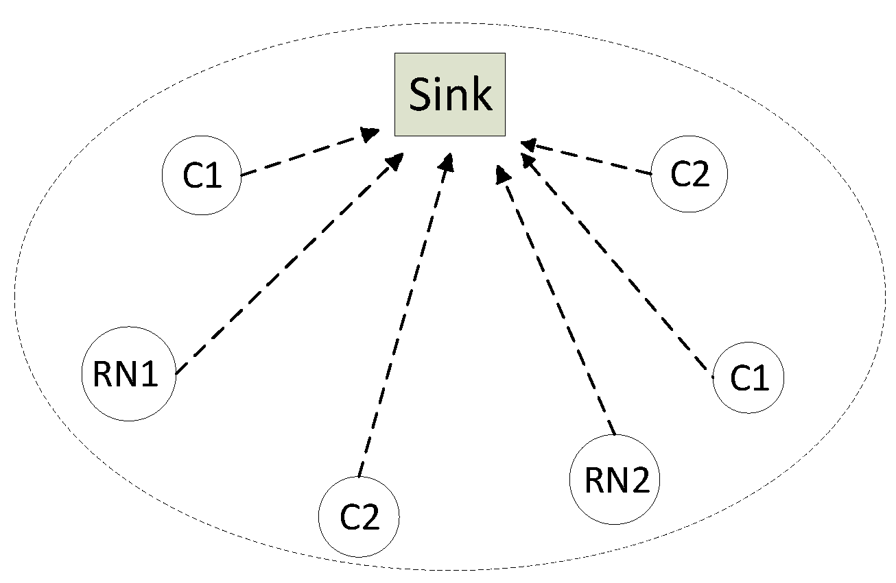
2.1. Network Assumptions

As a simplified example, the scenario under study is depicted in Figure 1. Two classes of SNs coexist in the WSN, $\mathrm{C}1$ and $\mathrm{C}2$ SNs. C1 SNs have priority over the C2 SNs for medium access. For modeling convenience, we arbitrarily select one SN from each class and refer to them as reference nodes, $\mathrm{RN}1$ and $\mathrm{RN}2$.

We focus on a single cell, where SNs are one hop away from each other. However, multiple cells together may form a larger network. SNs transmit packets towards a single destination node that we refer to as the sink. We assume that the sink node behaves as a packet absorption node, i.e., it only receives packets and never transmits them.

The network deploys the PSA-MAC protocol with the common CSMA/CA-based RTS/CTS/DATA/ACK packet handshake. SN that uses the PSA-MAC protocol perceive the time as partitioned into cycles, and each cycle is further divided into three parts (periods): sync, data and sleep. Also, we refer to the active period as the period of time composed by the aggregation of the sync and data periods. Backoff timers of active SNs that govern medium access are reset at each cycle initiation. In PSA-MAC, a SN goes to sleep until the next data period when: (i) it loses the contention (hears a busy medium before its backoff timer expires); (ii) it encounters an RTS collision; and (iii) after a successful transmission.

With aggregated packet transmission (APT), nodes might transmit a batch of DATA packets in a single cycle instead of a single one. We refer to the set of consecutive packets that will be transmitted together in the same cycle as a packet frame (PF). The maximum number of DATA packets that can be aggregated in a PF is constrained by the cycle duration T, the maximum frame length of the wireless link, by the number of DATA packets in the queue of the SN that gains access to the channel, and by a configurable parameter denoted by F, the maximum number of DATA packets that can be aggregated in a PF. SNs only transmit one PF per cycle. As an example of the operation of the AT scheme, assume that q is the number of DATA packets in the $\mathrm{RN}c$ queue, $c=1,2$. When $q\le F$, a successful PF transmission will empty its queue. However, when $q>F$, a successful PF transmission will leave $q-F$ DATA packets in its queue.

SNs are equipped with a battery, but energy harvesting is not supported [25]. In practical deployment scenarios, it has been shown that one or two retransmissions are sufficient to successfully send a PF [26,27]. Then, we consider an infinite retransmission model instead of the more complex finite retransmission one.

We assume that the number of DATA packets that arrive at the buffer of an SN follow a discrete Poisson distribution of mean $\lambda T$, where $\lambda$ is the DATA packet arrival rate and T is the cycle duration. However, the proposed analytical model is sufficiently general to accommodate any alternative discrete distribution. Each SN has a finite buffer size to hold up to Q DATA packets, Packets are served according to a FIFO discipline. From the MAC layer perception, we also assume that the channel is ideal (error-free).

Active SNs randomly select a backoff time with equal probability from the set $\left\{0,...,W-1\right\}$, where W is the length of the contention window, measured in backoff time slots. Consider that $\mathrm{RN}c$ from cluster $\mathrm{C}c$ is active, $c=1,2$. It transmits a PF successfully (without collision) if the other contending SNs from $\mathrm{C}c$ selected backoff times greater than the one chosen by the $\mathrm{RN}c$. A PF transmitted by $\mathrm{RN}c$ will fail (collide) when more than one contending SN from $\mathrm{C}c$ select the same backoff time as the $\mathrm{RN}c$, and the backoff time is the smallest among all contending SNs. When the backoff time generated by $\mathrm{RN}c$ is not the smallest one among those generated by the other contending SNs from $\mathrm{C}c$, two outcomes are possible: (i) another SN different from $\mathrm{RN}c$ can transmit successfully; (ii) other SNs different from $\mathrm{RN}c$ collide while transmitting. Please note that in the latter case, $\mathrm{RN}c$ will sense a busy medium before its backoff timer expires and will switch to the sleep mode. In these cycles, where $\mathrm{RN}c$ loses the contention, it wastes energy overhearing the channel. As shown later, the proposed model determines the amount of energy consumed by SNs due to overhearing.

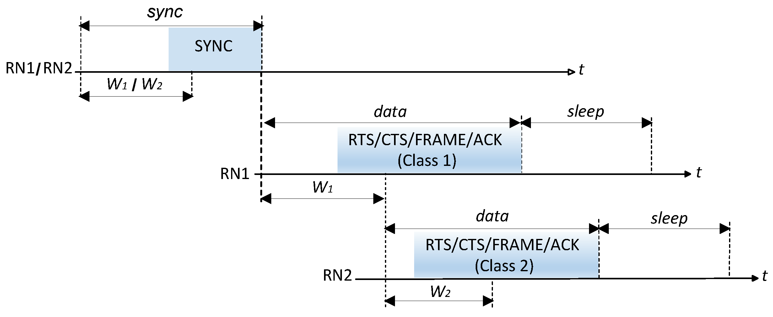
2.2. Transmission and Operation Modes

Figure 2 shows the medium access procedure for both SN classes over time. Observe that $\mathrm{C}1$ SNs are given medium access priority over $\mathrm{C}2$ SNs, by guaranteeing that $\mathrm{C}1$ SNs complete their medium access procedure before $\mathrm{C}2$ SNs do it. As the proposed methodology to determine the energy consumption takes into account the energy consumed during the sync period, the sync period for both SN classes is also shown in Figure 2.

The operation of an SN almost repeats every cycle and can be summarized as progressing along the following steps. First, SNs determine a sleep-wake up schedule during the sync period. To this end, SNs exchange SYNC packets among their neighbors. The next cycle initiation instant and the corresponding SN address are included in SYNC packets. SNs use this information to synchronize their wake up instants at the beginning of each sync period. Observe from Figure 2 that both SN classes deploy the same sync period.

Second, during the data period, the conventional CSMA/CA contention scheme is used to transmit PFs. Active nodes generate a random backoff time and perform common carrier sensing. If at backoff timer expiration, a SN senses an idle channel, it sends a PF using the RTS/CTS/DATA/ACK packet handshake. A PF is recognized as successfully transmitted when the SN receives an ACK from the sink.

Also, the energy consumed during the sleep period is taken into account. As mentioned above, during this period, nodes fall asleep to save energy or remain awake to listen to SYNC packets transmitted by other SNs.

Prioritization Scheme

As $\mathrm{C}1$ SNs have access priority over $\mathrm{C}2$ SNs, the data period is initiated and completed by active $\mathrm{C}1$ SNs first, if any. Active $\mathrm{C}2$ SNs wake up shortly after $\mathrm{C}1$ contention window ($W_1$) ends, and if they find an idle medium, $\mathrm{C}2$ SNs initiate their medium access contention. However, if active $\mathrm{C}2$ SNs sense a busy medium, they return to sleep mode and wake up again at the next cycle. We assume that the transmission time of the shortest $\mathrm{C}1$ PF (one DATA packet) exceeds $W_1$.

Please note that we assume that the energy consumed by $\mathrm{C}2$ SNs to sense a busy medium takes a single backoff time slot and, therefore, it is negligible. Note also that when $\mathrm{C}1$ SNs collide, $\mathrm{C}2$ SNs will also detect a busy medium, and they will refrain from contending in this cycle.

3. System Model

The system model that has been developed to evaluate the WSN performance was presented in [23,24]. The model considers a pair of coupled 2D-DTMCs, whose solution in terms of their stationary probability distributions is used to derive expressions that allow to compute of the energy consumption.

3.1. Medium Access

We denote by $N_1$ and $N_2$ the total number of SNs in each class. Let us assume that $\mathrm{RN}c$, $c=1,2$, is active in a given cycle, and let k denote the number of $\mathrm{C}c$ SNs, different from $\mathrm{RN}c$, that are also active in the same cycle, $0\le k\le N_c-1$. We denote by $P_{s,k,c}$, $P_{f,k,c}$, and $P_{sf,k,c}$, the probabilities that $\mathrm{RN}c$ transmits a PF successfully, with failure (collision), or just transmits a PF either with success or failure, respectively, when contending with other k$\mathrm{C}c$ SNs. Also, we denote by $B{T}_{s,k,c}$, and $B{T}_{f,k,c}$ the average backoff times generated by $\mathrm{RN}c$, conditioned on it transmits a PF with success or failure (collision), respectively, when contending with other k$\mathrm{C}c$ SNs. Please refer to [23] for details on how these parameters are determined.

3.2. Definition of the 2D-DTMCs

We propose a single 2D-DTMC per SN class to model the evolution of the state of nodes (active or inactive) and their queue lengths over time. More specifically, let $\left(i,m\right)$ be the state of an SN class, were i denotes the number of DATA packets in the corresponding RN queue, $0\le i\le Q$, and m denotes the number of active nodes of the class, different from the RN, $\left(m<N-1\right)$. Let $P_{(i,m),(j,n)}$ denote the transition probability from state $\left(i,m\right)$ to state $\left(j,n\right)$.

It is important to highlight that transition probabilities for each DTMC are substantially different from the ones defined in [23], as now they must take into account the fact that SNs might transmit multiple DATA packets (a PF) in a single cycle. For convenience, these new transition probabilities are defined in [28]. Please refer to this document for a detailed description of their definition.

We denote by $R_{1,0}$ the fraction of cycles in which all $\mathrm{C}1$ SNs are inactive and, therefore, there would be no PF transmissions from $\mathrm{C}1$ SNs. Clearly, $R_{1,0}$ is the fraction of cycles in which active $\mathrm{C}2$ SNs can contend for medium access. $R_{1,0}$ is the key coupling mechanism between the pair of DTMCs. The DTMC associated with $\mathrm{C}1$ SNs is independent from the one associated with $\mathrm{C}2$ SNs. Therefore, once the DTMC for $\mathrm{C}1$ is solved, $R_{1,0}$ can be determined and then, $\mathrm{C}2$ DTMC can be solved.

3.3. Solution of the 2D-DTMCs

Let ${\pi }_c\left(i,m\right)$ be the stationary probability of finding $\mathrm{C}c$ SNs in state $\left(i,m\right)$. That is, the fraction of cycles where $\mathrm{C}c$ SNs are in state $\left(i,m\right)$. Let ${\pi }_{\mathbf{c}}=\left[{\pi }_c(i,m)\right]$ be the stationary probability distribution. It can be obtained by iteratively solving the set of linear equations,

$${\mathit{\pi }}_{\mathit{c}}={\mathit{\pi }}_{\mathit{c}}{\mathit{P}}_{\mathit{c}},{\mathit{\pi }}_{\mathit{c}}\mathit{e}=\mathbf{1},$$

(1)

where ${\mathit{P}}_{\mathit{c}}=\left[P_{c,(i,m),(j,n)}\right]$ is the transition probability matrix of $\mathrm{C}c$, and $\mathbf{e}$ is a single column matrix of ones. Please note that transition probability matrices associated with $\mathrm{C}1$ and $\mathrm{C}2$ SNs, ${\mathit{P}}_{\mathbf{1}}$ and ${\mathit{P}}_{\mathbf{2}}$, respectively, contain different elements. This leads to different stationary probability distributions, ${\mathit{\pi }}_{\mathbf{1}}$ and ${\mathit{\pi }}_{\mathbf{2}}$, respectively. Please refer to [28] for a detailed description of the elements of ${\mathit{P}}_{\mathit{c}}$ and the iterative solution algorithm. Note that the elements of ${\mathit{P}}_{\mathbf{2}}$ are dependent on $R_{1,0}$.

4. Energy Consumption

In this section, we derive expressions to determine the average energy consumed by an RN per cycle, considering the different periods in which a cycle is divided as defined in Section 2.

We define an update supercycle as a set of $N_{sc}$ consecutive cycles. For simplicity, we assume that $\mathrm{C}c$ SNs transmit one SYNC packet every $N_{sc,c}$ cycles $c=1,2$, i.e., one SYNC packet per update supercycle. Also, they might receive one SYNC packet per cycle in the remaining $N_{sc,c}-1$ cycles. To avoid missing SYNC packets from neighboring nodes, occasionally, an SN keeps awake for a whole cycle. As these cycles are different from the normal cycles, which include a sleep period after an active period, we refer to them as awake cycles.

We define a hypercycle as a set of $N_{aw}$ consecutive update supercycles, i.e., $N_{aw}·N_{sc}$ consecutive cycles. We also assume that a $\mathrm{C}c$ SN follows awake cycles during a complete supercycle ($N_{sc,c}$ consecutive cycles), whereas it follows normal cycles during the other $N_{aw,c}-1$ update supercycles of the hypercycle. Clearly, these definitions of the normal and awake cycles have an impact on the energy consumed by an SN.

Only the energy consumed by the radio transceiver of an SN is considered by the model. The energy consumed due to the specific sensing tasks of SNs, being application-specific, has not been taken into account.

Along the next Sections we determine the energy consumed by $\mathrm{RN}1$ and $\mathrm{RN}2$. The energy consumed by any other node of the same class is the same as the one consumed by the corresponding RN.

4.1. Average Energy Consumed by $\mathrm{RN}c$ in the Sync Period

During the sync period, SNs exchange SYNC packets to synchronize their sleep-wake up schedules. The duration of the sync period for $\mathrm{C}c$ SNs can be determined as, $T_{sc,c}=(W_c-1)+t_{SYNC}+D_p$, where $W_c$ is the length of the contention window for $\mathrm{C}c$ SNs , $t_{SYNC}$ is the transmission time of a SYNC packet, and $D_p$ is the one-way propagation delay.

The average energy consumed by a $\mathrm{C}c$ SN during a sync period, $E_{s}c,c$, can be determined as,

$$\begin{array}{c}\hfill \begin{array}{cc}\hfill E_{sc,c}& ={\displaystyle \frac{1}{N_{sc,c}}}·\left[\left(t_{SYNC}·P_{tx,c}+\left(T_{sync,c}-t_{SYNC}\right)·P_{rx,c}\right)\right]+{\displaystyle \frac{N_{sc}-1}{N_{sc}}}·\left(T_{sync,c}·P_{rx,c}\right),\hfill \end{array}\end{array}$$

(2)

where $P_{t}x,c$ and $P_{r}x,c$ are the transmission and reception power levels for $\mathrm{C}c$ SNs, respectively.

4.2. Average Energy Consumed by $\mathrm{RN}1$ in the Data Period

The average energy consumed by $\mathrm{RN}1$ while being active in a data period is composed of different terms, each of which depends on the possible outcomes of the contention process: (i) it completes a successful PF transmission, $E_{tx,s}^{d,1}$ ; (ii) a PF transmitted by $\mathrm{RN}1$ collides, $E_{tx,f}^{d,1}$ ; (iii) one or more $\mathrm{C}1$ SNs, different from $\mathrm{RN}1$, win the contention and transmit a PF, $E_{oh}^{d,1}$. In the last case, the $\mathrm{RN}1$ will sense a busy channel before its backoff timer expires, and it will switch to the sleep mode. However, it has been listening to the channel (overhearing) until detecting it was busy, and this wasted energy consumption must be taken into account.

$$\begin{array}{cc}\hfill E_{tx,s}^{d,1}& =\sum _{i=1}^{Q_1}\sum _{k=0}^{M_1}{\pi }_1\left(i,k\right)P_{s,k,1}\left(E_1^{d,1}+B{T}_{s,k,1}{P}_{rx,1}+{\alpha }_1{t}_{DATA}{P}_{tx,1}\right),\hfill \\ \hfill E_1^{d,1}& =t_{RTS}{P}_{tx,1}+\left[t_{CTS}+t_{ACK}+4D_p\right]P_{rx,1},\hfill \\ \hfill {\alpha }_1& =min\left(i,F_1\right).\hfill \end{array}$$

(3)

where $Q_1$ is $\mathrm{RN}1$ buffer size in DATA packets, $M_1=N_1-1$ is the number of $\mathrm{C}1$ SNs different from $\mathrm{RN}1$, ${\alpha }_1$ is the number of DATA packets aggregated in the current PF, $F_1$ is the maximum number of DATA packets that $\mathrm{C}1$ SNs can aggregate, $t_{R}TS,t_{D}ATA,t_{C}TS$, and $t_{A}CK$ are the transmission times of the corresponding packets, and $P_{s,k,1}$ and $B{T}_{s,k,1}$ were already defined in Section 3.1.

$$\begin{array}{cc}\hfill E_{tx,f}^{d,1}& =\sum _{i=1}^{Q_1}\sum _{k=0}^{M_1}{\pi }_1(i,k)P_{f,k,1}\left(E_2^{d,1}+B{T}_{f,k,1}{P}_{rx,1}\right),\hfill \\ \hfill E_2^{d,1}& =t_{RTS}{P}_{tx,1}+2D_p{P}_{rx,1}.\hfill \end{array}$$

(4)

$$\begin{array}{c}\hfill \begin{array}{cc}\hfill E_{oh}^{d,1}& =\sum _{i=1}^{Q_1}\sum _{k=1}^{M_1}{\pi }_1(i,k)k{P}_{s,k,1}\left[B{T}_{s,k,1}+t_{RTS}\right]P_{rx,1}\hfill \\ \hfill & +\sum _{i=1}^{Q_1}\sum _{k=2}^{M_1}{\pi }_1(i,k){\widehat{P}}_{f,k,1}B{T}_{f,k,1}{P}_{rx,1},\hfill \\ \hfill {\widehat{P}}_{f,k,1}& =\sum _{i=1}^{W_1}\left[\sum _{n=2}^k\left({\displaystyle \genfrac{}{}{0pt}{}{k}{n}}\right){\left({\displaystyle \frac{1}{W_1}}\right)}^n{\left({\displaystyle \frac{W_1-i}{W_1}}\right)}^{k-n+1}\right].\hfill \end{array}\end{array}$$

(5)

where ${\widehat{P}}_{f,k,1}$ is the probability that PFs transmitted by other SNs different from $\mathrm{RN}1$ collide, in a cycle where $\mathrm{RN}1$ is active but loses the contention, and $P_{f,k,1}$ and $B{T}_{f,k,1}$ were already defined in Section 3.1.

The average energy consumed by $\mathrm{RN}1$ along the data period of a cycle can be determined as

$$\begin{array}{cc}\hfill E_{d,1}& =E_{tx,s}^{d,1}+E_{tx,f}^{d,1}+E_{oh}^{d,1}.\hfill \end{array}$$

(6)

4.3. Average Energy Consumed by $\mathrm{RN}2$ in the Data Period

For $\mathrm{RN}2$, the average energy it consumes along the data period of a cycle can be expressed as,

$$\begin{array}{cc}\hfill E_{d,2}& =\left(E_{tx,s}^{d,2}+E_{tx,f}^{d,2}+E_{oh}^{d,2}\right)R_{1,0}.\hfill \end{array}$$

(7)

where $E_{tx,s}^{d,2}$, $E_{tx,f}^{d,2}$ and $E_{oh}^{d,2}$ have the same terms as those shown in (3)–(5), but appropriately adapted for the specific features of $\mathrm{C}2$ SNs.

4.4. Average Energy Consumed by $\mathrm{RN}1$ during Awake Cycles

When $\mathrm{RN}1$ is in awake mode, it wakes up at the beginning of awake cycles and remains awake until the cycle ends. During awake cycles, $\mathrm{RN}1$ listens to the channel for the possible transmission of SYNC packets from neighboring SNs. For energy conservation, when $\mathrm{RN}1$ hears a RTS packet, indicating the beginning of a PF transmission, it calculates the time the channel will remain occupied from the information contained in the RTS packet, and switches to the sleep mode. When the PF transmission ends, it returns to the awake state.

We now determine the average energy consumed by $\mathrm{RN}1$ per awake cycle. It is assumed that SNs activate the awake mode at the beginning of the data period, i.e., once the sync period ends. For the average energy consumed by $\mathrm{RN}1$ per awake cycle, we consider two terms: (i) the energy consumed due to the channel listening activity; (ii) the energy consumed due to being in the sleep mode while other SNs occupy the channel.

We consider the following cycle types:

• Cycle 1A: $\mathrm{RN}1$ is active, $\left(i_1>0,k_1\ge 0\right)$.
• Zero or more $\mathrm{C}1$ SNs might also be active. When other SNs are active, in addition to $\mathrm{RN}1$, the following contention outcomes are possible: (i) $\mathrm{RN}1$ completes a successful PF transmission; (ii) the PF from $\mathrm{RN}1$ collides; (iii) another node completes a successful PF transmission, and (iv) other nodes different from $\mathrm{RN}1$ collide.
• Cycle 1B: $\mathrm{RN}1$ is inactive, $\left(i_1=0,k_1>0\right)$.
• $\mathrm{C}1$ SNs access the channel while $\mathrm{RN}1$ is awake. $\mathrm{RN}1$ listens to the channel to decode the RTS packet and determine the duration of the PF transmission. The following contention outcomes are possible: (i) a SN completes a successful PF transmission; (ii) multiple PFs collide.
• Cycle 1C: All $\mathrm{C}1$ SNs remain inactive, including $\mathrm{RN}1$, $(i_1=0,k_1=0)$.
• There are active $\mathrm{C}2$ SNs that access the channel while $\mathrm{RN}1$ is awake, $(i_2>0,k_2>0)$. $\mathrm{RN}1$ listens to the channel, decodes the RTS packets in collision-free cycles and determines the duration of the PF transmissions. The following contention outcomes for $\mathrm{C}2$ SNs might be possible: (i) a $\mathrm{C}2$ SN completes a successful PF transmission; (ii) multiple PFs from different $\mathrm{C}2$ SNs collide.
• Cycle 1D: All $\mathrm{C}1$ and $\mathrm{C}2$ SNs remain inactive, $i_1=k_1=i_2=k_2=0$, while $\mathrm{RN}1$ is awake.

4.4.1. Average Energy Consumed by $\mathrm{RN}1$ in Type 1A Cycles

Let $E_{tx,s}^{aw}\left[1A\right]$, $E_{tx,f}^{aw}\left[1A\right]$ and $E_{oh}^{aw}\left[1A\right]$ be the average energy consumed by $\mathrm{RN}1$ in type 2A cycles when $\mathrm{RN}1$ completes a successful PF transmission, a PF from $\mathrm{RN}1$ collides, and $\mathrm{RN}1$ overhears PF transmissions from other $\mathrm{C}1$ SNs, respectively.

These $\mathrm{RN}1$ energy consumption terms can be determined as,

$$\begin{array}{c}\hfill \begin{array}{cc}\hfill E_{tx,s}^{aw}\left[1A\right]& =\sum _{i=1}^{Q_1}\sum _{k=1}^{M_1}{\pi }_1(i,k)P_{s,k,1}\left[E_1^{aw,1}-\left(B{T}_{s,k,1}+{\alpha }_1{t}_{DATA}\right)P_{rx,1}\right],\hfill \\ \hfill E_1^{aw,1}& =\left[T-T_{sc,1}-\left(t_{RTS}+t_{CTS}+t_{ACK}+4D_p\right)\right]P_{rx,1}.\hfill \end{array}\end{array}$$

(8)

$$\begin{array}{c}\hfill \begin{array}{cc}\hfill E_{tx,f}^{aw}\left[1A\right]& =\sum _{i=1}^{Q_1}\sum _{k=1}^{M_1}{\pi }_1(i,k)P_{f,k,1}\left[E_2^{aw,1}-B{T}_{f,k,1}{P}_{rx,1}\right],\hfill \\ \hfill E_2^{aw,1}& =\left[T-T_{sc,1}-\left(t_{RTS}+2D_p\right)\right]P_{rx,1}.\hfill \end{array}\end{array}$$

(9)

$$\begin{array}{c}\hfill \begin{array}{cc}\hfill E_{oh}^{aw}\left[1A\right]& =\sum _{i=1}^{Q_1}\sum _{k=1}^{M_1}{\pi }_1(i,k)k{P}_{s,k,1}\left[E_3^{aw,1}-{\widehat{f}}_{k,1}{t}_{DATA}\left(P_{rx,1}-P_{sl}\right)\right]\hfill \\ \hfill & +\sum _{i=1}^{Q_1}\sum _{k=2}^{M_1}{\pi }_1(i,k){\widehat{P}}_{f,k,1}\left(T-T_{sc,1}\right)P_{rx,1},\hfill \\ \hfill E_3^{aw,1}& =\left(T-T_{sc,1}\right)P_{rx,1}-\left(t_{CTS}+t_{ACK}+3D_p\right)\left(P_{rx,1}-P_{sl}\right),\hfill \\ \hfill {\widehat{P}}_{f,k,1}& =\sum _{i=1}^{W_1}\left[\sum _{n=2}^k\left({\displaystyle \genfrac{}{}{0pt}{}{k}{n}}\right){\left({\displaystyle \frac{1}{W_1}}\right)}^n{\left({\displaystyle \frac{W_1-i}{W_1}}\right)}^{k-n+1}\right],\hfill \\ \hfill {\widehat{f}}_{k,1}& ={\displaystyle \frac{1}{G_{k,1}}}\sum _{i=1}^{Q_1}{\alpha }_1·{\pi }_1(i,k),10.0mu{G}_{k,1}=\sum _{i=1}^{Q_1}{\pi }_1(i,k).\hfill \end{array}\end{array}$$

(10)

where T is the cycle duration, ${\widehat{P}}_{f,k,1}$ is the probability that PFs transmitted by other SNs, different from $\mathrm{RN}1$, collide in cycles where $\mathrm{RN}1$ is active but loses the contention, ${\widehat{f}}_{k,1}$ is the average PF size transmitted by $\mathrm{C}1$ SNs, conditioned on $\mathrm{RN}1$ being contending with other k$\mathrm{C}1$ SNs in the same cycle, and $P_{s}l$ is the power level in sleep mode [23]. Please note that ${\widehat{f}}_{k,1}$ is obtained to determine the average time that $\mathrm{RN}1$ will remain in the sleep mode awaiting the end of the PF transmission. Note also that ${\widehat{f}}_{k,1}=1$ when the SPT scheme is deployed.

Then, the average energy consumed by $\mathrm{RN}1$ in type 1A awake cycles is

$$\begin{array}{c}\hfill \begin{array}{cc}\hfill E_{aw}\left[1A\right]& =E_{tx,s}^{aw}\left[1A\right]+E_{tx,f}^{aw}\left[1A\right]+E_{oh}^{aw}\left[1A\right].\hfill \end{array}\end{array}$$

(11)

4.4.2. Average Energy Consumed by $\mathrm{RN}1$ in Type 1B Cycles

The average energy consumed by $\mathrm{RN}1$ in type 1B awake cycles can be determined as

$$\begin{array}{c}\hfill \begin{array}{cc}\hfill E_{aw}\left[1B\right]& =\sum _{k=1}^{M_1}{\pi }_1(0,k)k{P}_{s,k-1,1}\left[E_3^{aw,1}-{\widehat{f}}_{k-1,1}{t}_{DATA}\left(P_{rx,1}-P_{sl}\right)\right]\hfill \\ \hfill & +\sum _{k=2}^{M_1}{\pi }_1(0,k){\widehat{P}}_{f,k,1}^{\prime }\left(T-T_{sc,1}\right)P_{rx,1},\hfill \\ \hfill {\widehat{P}}_{f,k,1}^{\prime }& =\sum _{i=1}^{W_1}\left[\sum _{n=2}^k\left({\displaystyle \genfrac{}{}{0pt}{}{k}{n}}\right){\left({\displaystyle \frac{1}{W_1}}\right)}^n{\left({\displaystyle \frac{W_1-i}{W_1}}\right)}^{k-n}\right],\hfill \end{array}\end{array}$$

(12)

where ${\widehat{P}}_{f,k,1}^{\prime }$ denotes the probability that two or more of the k SNs, other than $\mathrm{RN}1$, transmit with collision while $\mathrm{RN}1$ is inactive. Please note that ${\widehat{f}}_{k-1,1}$ can be obtained as in (10).

4.4.3. Energy Consumption in Type 1C Cycles

The energy consumed by $\mathrm{RN}1$ in type 1C awake cycles can be determined as

$$\begin{array}{c}\hfill \begin{array}{cc}\hfill E_{aw}\left[1C\right]& =\sum _{i=1}^{Q_2}\sum _{k=1}^{M_2}{\pi }_2(i,k)\left(k+1\right)P_{s,k,2}\left[E_3^{aw,1}-{\widehat{f}}_{k,2}{t}_{DATA}\left(P_{rx,1}-P_{sl}\right)\right]\hfill \\ \hfill & +\sum _{k=1}^{M_2}{\pi }_2(0,k)k{P}_{s,k-1,2}\left[E_3^{aw,1}-{\widehat{f}}_{k-1,2}{t}_{DATA}\left(P_{rx,1}-P_{sl}\right)\right]\hfill \\ \hfill & +\sum _{i=1}^{Q_2}\sum _{k=2}^{M_2}{\pi }_2(i,k){\widehat{P}}_{f,k,2}\left(T-T_{sc,1}c\right)P_{rx,1}\hfill \\ \hfill & +\sum _{k=2}^{M_2}{\pi }_2(0,k){\widehat{P}}_{f,k,2}^{\prime }\left(T-T_{sc,1}\right)P_{rx,1},\hfill \\ \hfill {\widehat{f}}_{k,2}& ={\displaystyle \frac{1}{G_{k,2}}}\sum _{i=1}^{Q_2}{\alpha }_1·{\pi }_2(i,k),10.0mu{G}_{k,2}=\sum _{i=1}^{Q_2}{\pi }_2(i,k).\hfill \end{array}\end{array}$$

(13)

where ${\widehat{P}}_{f,k,2}$ is the probability that PFs transmitted by $\mathrm{RN}2$ collide while contending with other additional k$\mathrm{C}2$ SNs, ${\widehat{P}}_{f,k,2}^{\prime }$ is the probability that two or more of the k active SNs, other than $\mathrm{RN}2$, transmit with collision while $\mathrm{RN}2$ is inactive, ${\widehat{f}}_{k,2}$ is the average PF size transmitted by $\mathrm{RN}2$, conditioned on $\mathrm{RN}2$ being contending with other k$\mathrm{C}2$ SNs in the same cycle, ${\alpha }_2=min(i,F_2)$ is the number of DATA packets aggregated in the current PF, $F_1$ is the maximum number of DATA packets that $\mathrm{C}2$ SNs can aggregate, ${\widehat{P}}_{f,k,2}$, ${\widehat{P}}_{f,k,2}^{\prime }$, ${\widehat{f}}_{k,2}$ and ${\widehat{f}}_{k-1,2}$ can be determined in the same way as their $\mathrm{C}1$ counterparts.

As before, note that ${\widehat{f}}_{k,2}$${\widehat{f}}_{k-1,2}$ are obtained to determine the average time $\mathrm{RN}1$ will remain in the sleep mode while waiting for the end of the PF transmitted by a $\mathrm{C}2$ SNs. Note also that ${\widehat{f}}_{k,2}=1$ when the SPT scheme is deployed.

Each of the terms in expression (13) defines the average energy consumed by $\mathrm{RN}1$ due to the occurrence of different events. The first term accounts for the average energy consumed when one of the $k+1$ active $\mathrm{C}2$ SNs (the $\mathrm{RN}2$ and other k$\mathrm{C}2$ SNs) transmits a PF successfully. The second term accounts for the average energy consumed when one of the k active $\mathrm{C}2$ SNs other than $\mathrm{RN}2$, transmits a PF successfully in a cycle where $\mathrm{RN}2$ is inactive. The third and fourth account for the average energy consumed when two or more of k$\mathrm{C}2$ SNs, different from the $\mathrm{RN}2$, transmit with collision when the $\mathrm{RN}2$ is active or inactive, respectively.

4.4.4. Energy Consumption in in Type 1D Cycles

The average energy consumed by $\mathrm{RN}1$ in type 1D awake cycles can be determined as

$$\begin{array}{c}\hfill \begin{array}{c}\hfill E_{aw}\left[1D\right]={\pi }_1(0,0){\pi }_2(0,0)\left(T-T_{sc,1}\right)P_{rx,1}.\end{array}\end{array}$$

(14)

4.4.5. Average Energy Consumed by $\mathrm{RN}1$ in awake Cycles

The total average energy consumed by $\mathrm{RN}1$ in awake cycles can be determined as

$$\begin{array}{c}\hfill \begin{array}{cc}\hfill E_{aw,1}& =E_{aw}\left[1A\right]+E_{aw}\left[1B\right]+R_{1,0}{E}_{aw}\left[1C\right]+E_{aw}\left[1D\right],\hfill \\ \hfill E_{aw,1}& =E_{tx,s}^{aw}\left[1A\right]+E_{tx,f}^{aw}\left[1A\right]+E_{oh}^{aw}\left[1A\right]+E_{aw}\left[1B\right]+R_{1,0}{E}_{aw}\left[1C\right]+E_{aw}\left[1D\right].\hfill \end{array}\end{array}$$

(15)

Please note that $E_{aw}\left[1C\right]$ is weighted by the fraction of cycles where $\mathrm{C}1$ SNs remain inactive, $R_{1,0}$. In these cycles, active $\mathrm{C}2$ SNs, if any, will contend for medium access.

4.5. Average Energy Consumed by $\mathrm{RN}2$ during Awake Cycles

As the operation of $\mathrm{RN}1$ and $\mathrm{RN}2$ during awake cycles is similar, please refer to Section 4.4 for the operational specific details. We now determine the average energy consumed by $\mathrm{RN}2$ per awake cycle. We consider two terms: (i) the energy consumed due to the channel listening activity; (ii) the energy consumed due to being in the sleep mode while other SNs occupy the channel.

We identify the following cycle types:

• Cycle 2A: $\mathrm{C}1$ SNs are inactive $\left(i_1=0,k_1=0\right)$, but $\mathrm{RN}2$ and other $\mathrm{C}2$ SNs are active $\left(i_2>0,k_2\ge 0\right)$. Either $\mathrm{RN}2$ or any other active $\mathrm{C}2$ SNs will access the channel, while $\mathrm{RN}2$ is awake in the same cycle. The possible contention outcomes are: (a) $\mathrm{RN}2$ successfully transmits a PF; (b) a PF transmitted by $\mathrm{RN}2$ collides; (c) another $\mathrm{C}2$ SN successfully transmits a PF; (d) other $\mathrm{C}2$ SNs collide.
• Cycle 2B: $\mathrm{C}1$ SNs are inactive, $\mathrm{RN}2$ is also inactive, but other $\mathrm{C}2$ SNs are active, $\left(i_2=0,k_2>0\right)$. $\mathrm{C}2$ SNs access the channel in the same cycle that $\mathrm{RN}2$ is awake. The possible contention outcomes are: (a) a $\mathrm{C}2$ SN successfully transmits a PF; (b) multiple $\mathrm{C}2$ SNs collide.
• Cycle 2C: All $\mathrm{C}1$ SNs are active, $\left(i_1\ge 0,k_1\ge 0\right)$, while $\mathrm{C}2$ SNs, including $\mathrm{RN}1$ SNs, are inactive, $\left(i_2=0,k_2=0\right)$. The possible contention outcomes are: (a) a $\mathrm{C}1$ SN successfully transmits a PF; (b) multiple $\mathrm{C}1$ SNs collide.
• Cycle 2D: $\mathrm{RN}2$ and the rest of $\mathrm{C}1$ and $\mathrm{C}2$ SNs are inactive, $i_1=k_1=i_2=k_2=0$. Please note that in cycles of type 2D, both $\mathrm{RN}1$ and $\mathrm{RN}2$ might simultaneously coincide in their respective awake cycles.

4.5.1. Energy Consumption in Type 2A Cycles

Let $E_{tx,s}^{aw}\left[2A\right]$, $E_{tx,f}^{aw}\left[2A\right]$ and $E_{oh}^{aw}\left[2A\right]$, be the average energy consumed by $\mathrm{RN}2$ in type 1A cycles when $\mathrm{RN}2$ completes a successful PF transmission, a PF from $\mathrm{RN}2$ collides, and $\mathrm{RN}2$overhears a PF transmission from other $\mathrm{C}2$ SNs, respectively.

These $\mathrm{RN}2$ energy consumption terms can be determined as,

$$\begin{array}{c}\hfill \begin{array}{cc}\hfill E_{tx,s}^{aw}\left[2A\right]& =\sum _{i=1}^{Q_2}\sum _{k=1}^{N_2}{\pi }_2(i,k)P_{s,k,2}\left[E_1^{aw,2}-\left({\alpha }_2{t}_{DATA}+B{T}_{s,k,2}\right)P_{rx,2}\right],\hfill \\ \hfill E_1^{aw,2}& =\left[T-T_{sc,2}-\left(t_{RTS}+t_{CTS}+t_{ACK}+4D_p\right)\right]P_{rx,2},\hfill \\ \hfill {\alpha }_2& =min(i,F_2).\hfill \end{array}\end{array}$$

(16)

$$\begin{array}{c}\hfill \begin{array}{cc}\hfill E_{tx,f}^{aw}\left[2A\right]& =\sum _{i=1}^{Q_2}\sum _{k=1}^{N_2}{\pi }_2(i,k)P_{f,k,2}\left[E_2^{aw,2}-B{T}_{f,k,2}{P}_{rx,2}\right],\hfill \\ \hfill E_2^{aw,2}& =\left[T-T_{sc,2}-\left(t_{RTS}+2D_p\right)\right]P_{rx,2}.\hfill \end{array}\end{array}$$

(17)

$$\begin{array}{c}\hfill \begin{array}{cc}\hfill E_{oh}^{aw}\left[2A\right]& =\sum _{i=1}^{Q_2}\sum _{k=1}^{N_2}{\pi }_2(i,k)k{P}_{s,k,2}\left[E_3^{aw,2}-{\widehat{f}}_{k,2}{t}_{DATA}\left(P_{rx,2}-P_{sl}\right)\right]\hfill \\ \hfill & +\sum _{i=1}^{Q_2}\sum _{k=2}^{N_2}{\pi }_2(i,k){\widehat{P}}_{f,k,2}\left(T-T_{sc,2}\right)P_{rx,2},\hfill \\ \hfill E_3^{aw,2}& =\left(T-T_{sc,2}\right)P_{rx,2}-\left(t_{CTS}+t_{ACK}+3D_p\right)\left(P_{rx,2}-P_{sl}\right).\hfill \end{array}\end{array}$$

(18)

where ${\alpha }_2$, $F_2$, ${\widehat{P}}_{f,k,2}$ and ${\widehat{f}}_{k,2}$ have identical meaning and purpose than their $\mathrm{C}1$ counterparts defined in (10).

Then, the average energy consumed by $\mathrm{RN}2$ in type 1A awake cycles is,

$$\begin{array}{c}\hfill \begin{array}{cc}\hfill E_{aw}\left[2A\right]& =E_{tx,s}^{aw}\left[2A\right]+E_{tx,f}^{aw}\left[2A\right]+E_{oh}^{aw}\left[2A\right].\hfill \end{array}\end{array}$$

(19)

4.5.2. Energy Consumption in Type 2B Cycles

The average energy consumed by $\mathrm{RN}2$ in type 2B awake cycles can be determined as

$$\begin{array}{c}\hfill \begin{array}{cc}\hfill E_{aw}\left[2B\right]& =\sum _{k=1}^{N_2}{\pi }_2(0,k)k{P}_{s,k-1,2}\left[E_3^{aw,2}-{\widehat{f}}_{k-1,2}{t}_{DATA}\left(P_{rx,2}-P_{sl}\right)\right]\hfill \\ \hfill & +\sum _{k=2}^{N_2}{\pi }_2(0,k){\widehat{P}}_{f,k,2}^{\prime }\left(T-T_{sc,2}\right)P_{rx,2}.\hfill \end{array}\end{array}$$

(20)

where, as for $\mathrm{C}1$ SNs, ${\widehat{P}}_{f,k,2}^{\prime }$ is the probability that one of the k$\mathrm{C}2$ SNs, different from $\mathrm{RN}2$, transmits a PF with collision when $\mathrm{RN}2$ is inactive.

4.5.3. Energy Consumption in Type 2C Cycles

The average energy consumed by $\mathrm{RN}2$ in type 2C awake cycles can be determined as

$$\begin{array}{c}\hfill \begin{array}{cc}\hfill E_{aw}\left[2C\right]& =\sum _{i=1}^{Q_1}\sum _{k=1}^{N_1}{\pi }_1(i,k)\left(k+1\right)P_{s,k,1}\left[E_3^{aw,2}-{\widehat{f}}_{k,1}{t}_{DATA}\left(P_{rx,2}-P_{sl}\right)\right]\hfill \\ \hfill & +\sum _{k=1}^{N_1}{\pi }_1(0,k)k{P}_{s,k-1,1}\left[E_3^{aw,2}-{\widehat{f}}_{k-1,1}{t}_{DATA}\left(P_{rx,2}-P_{sl}\right)\right]\hfill \\ \hfill & +\sum _{i=1}^{Q_1}\sum _{k=2}^{N_1}{\pi }_1(i,k){\widehat{P}}_{f,k,1}\left(T-T_{sc,2}\right)P_{rx,2}\hfill \\ \hfill & +\sum _{k=2}^{N_1}{\pi }_1(0,k){\widehat{P}}_{f,k,1}^{\prime }\left(T-T_{sc,2}\right)P_{rx,2}.\hfill \end{array}\end{array}$$

(21)

The type of events associated with the different terms in the expression above have the same meaning and purpose as their $\mathrm{C}1$ counterparts, that were described in Section 4.4.3.

4.5.4. Energy Consumption in Type 2D Cycles

The average energy consumed by $\mathrm{RN}2$ in type 2D awake cycles can be determined as

$$\begin{array}{c}\hfill \begin{array}{c}\hfill E_{aw}\left[2D\right]={\pi }_1(0,0){\pi }_2(0,0)\left(T-T_{sc,2}\right)P_{rx,2}.\end{array}\end{array}$$

(22)

4.5.5. Average Energy Consumed by $\mathrm{RN}2$ in Awake Cycles

The total average energy consumed by $\mathrm{RN}2$ in awake cycles can be determined as

$$\begin{array}{c}\hfill \begin{array}{cc}\hfill E_{aw,2}& =\left(E_{aw}\left[2A\right]+E_{aw}\left[2B\right]\right)R_{1,0}+E_{aw}\left[2C\right]+E_{aw}\left[2D\right],\hfill \\ \hfill E_{aw,2}& =\left(E_{tx,s}^{aw}\left[2A\right]+E_{tx,f}^{aw}\left[2A\right]+E_{oh}^{aw}\left[2A\right]+E_{aw}\left[2B\right]\right)R_{1,0}\hfill \\ \hfill & +E_{aw}\left[2C\right]+E_{aw}\left[2D\right].\hfill \end{array}\end{array}$$

(23)

Observe that $E_{aw}\left[2A\right]$ and $E_{aw}\left[2B\right]$ are weighted by $R_{1,0}$, the fraction of cycles where $\mathrm{C}1$ SNs are inactive.

4.6. Average Energy Consumption during Normal Cycles

Recall that after a successful or failed PF transmission, SNs switch to the sleep mode during the rest of the cycle to save energy. We refer to these cycles as normal cycles. In this subsection, we determine the average energy consumed by an RN in a normal cycle exclusively due to being in the sleep mode.

4.6.1. $\mathrm{C}1$ Sensor Nodes

The average energy consumed by $\mathrm{RN}1$ in a normal cycle can be expressed as being composed of different terms, each of them depends on the possible outcomes of the $\mathrm{RN}1$ contention process: (i) it completes a successful PF transmission, $E_{tx,s}^{nr,1}$ ; (ii) a PF transmitted by $\mathrm{RN}1$ collides, $E_{tx,f}^{nr,1}$ ; (iii) one or more $\mathrm{C}1$ SNs, different from $\mathrm{RN}1$, win the contention and transmit a PF, $E_{oh}^{nr,1}$.

$$\begin{array}{c}\hfill \begin{array}{cc}\hfill E_{tx,s}^{nr,1}& =\sum _{i=1}^{Q_1}\sum _{k=0}^{M_1}{\pi }_1\left(i,k\right)P_{s,k,1}{T}_1^{nr,1}{P}_{sl},\hfill \\ \hfill T_1^{nr,1}& =T-T_{sc,1}-\left(B{T}_{s,k,1}+t_{RTS}+{\alpha }_1{t}_{DATA}+t_{CTS}+t_{ACK}+4D_p\right),\hfill \\ \hfill {\alpha }_1& =min(i,F_1).\hfill \end{array}\end{array}$$

(24)

$$\begin{array}{c}\hfill \begin{array}{cc}\hfill E_{tx,f}^{nr,1}& =\sum _{i=1}^{Q_1}\sum _{k=1}^{M_1}{\pi }_1\left(i,k\right)P_{f,k,1}{T}_2^{nr,1}{P}_{sl},\hfill \\ \hfill T_2^{nr,1}& =T-T_{sc,1}-\left(B{T}_{f,k,1}+t_{RTS}+D_p\right)..\hfill \end{array}\end{array}$$

(25)

$$\begin{array}{c}\hfill \begin{array}{cc}\hfill E_{oh}^{nr,1}& =\sum _{i=1}^{Q_1}\sum _{k=1}^{M_1}{\pi }_1\left(i,k\right)k{P}_{s,k,1}\left(T_3^{nr,1}-B{T}_{s,k,1}\right)P_{sl}\hfill \\ \hfill & +\sum _{i=1}^{Q_1}\sum _{k=2}^{M_1}{\pi }_1\left(i,k\right){\widehat{P}}_{f,k,1}\left(T_3^{nr,1}-B{T}_{f,k,1}\right)P_{sl}\hfill \\ \hfill & +\sum _{k=0}^{M_1}{\pi }_1\left(0,k\right)\left(T-T_{sc,1}\right)P_{sl},\hfill \\ \hfill T_3^{nr,1}& =T-T_{sc,1}-\left(t_{RTS}+D_p\right).\hfill \end{array}\end{array}$$

(26)

The average energy consumed by $\mathrm{RN}1$ in a normal cycles can be expressed as,

$$\begin{array}{cc}\hfill E_{nr,1}& =E_{tx,s}^{nr,1}+E_{tx,f}^{nr,1}+E_{oh}^{nr,1}.\hfill \end{array}$$

(27)

4.6.2. $\mathrm{C}2$ Sensor Nodes

The average energy consumed by $\mathrm{RN}2$ in a normal cycle can be expressed as being composed of different terms, each of them associated with the occurrence of the possible outcomes of the $\mathrm{RN}2$ contention process. $\mathrm{RN}2$ switches to sleep mode when any of the following events occur: (i) $\mathrm{RN}2$ completes the transmission of a PF with success, $E_{tx,s}^{nr,2}$ ; (ii) $\mathrm{RN}2$ detects a collision when transmitting a PF, $E_{tx,f}^{nr,2}$ ; (iii) an active $\mathrm{RN}2$ detects that it has lost the contention with other $\mathrm{C}2$ SNs, $E_{oh}^{nr,2}$ ; (iv) in cycles in which all $\mathrm{C}2$ are inactive, $E_{id}^{nr,2}$. (v) along any cycles in which $\mathrm{C}1$ SNs access the channel and, therefore, the medium is busy for $\mathrm{C}2$ SNs, $E_{bm}^{nr,2}$ ;

$$\begin{array}{c}\hfill \begin{array}{cc}\hfill E_{tx,s}^{nr,2}& =\sum _{i=1}^{Q_2}\sum _{k=0}^{M_2}{\pi }_2\left(i,k\right)P_{s,k,2}\left[T_1^{nr,2}-\left(B{T}_{s,k,2}+{\alpha }_2{t}_{DATA}\right)\right]P_{sl}{R}_{1,0},\hfill \\ \hfill T_1^{nr,2}& =T-T_{sc,2}-\left(t_{RTS}+t_{CTS}+t_{ACK}+4D_p\right),\hfill \\ \hfill {\alpha }_2& =min(i,F_2).\hfill \end{array}\end{array}$$

(28)

$$\begin{array}{c}\hfill \begin{array}{cc}\hfill E_{tx,f}^{nr,2}& =\sum _{i=1}^{Q_2}\sum _{k=1}^{M_2}{\pi }_2\left(i,k\right)P_{f,k,2}\left[T_2^{nr}-B{T}_{f,k,2}\right]P_{sl}{R}_{1,0},\hfill \\ \hfill T_2^{nr,2}& =T-T_{sc,2}-\left(t_{RTS}+2D_p\right).\hfill \end{array}\end{array}$$

(29)

$$\begin{array}{c}\hfill \begin{array}{cc}\hfill E_{oh}^{nr,2}& =\sum _{i=1}^{Q_2}\sum _{k=1}^{M_2}{\pi }_2\left(i,k\right)k{P}_{s,k,2}\left(T_3^{nr,2}-B{T}_{s,k,2}\right)P_{sl}{R}_{1,0}\hfill \\ \hfill & +\sum _{i=1}^{Q_2}\sum _{k=2}^{M_2}{\pi }_2\left(i,k\right){\widehat{P}}_{f,k,2}+\left(T_3^{nr,2}-B{T}_{f,k,2}\right)P_{sl}{R}_{1,0},\hfill \\ \hfill T_3^{nr,2}& =T-T_{sc,2}-t_{RTS}-D_p.\hfill \end{array}\end{array}$$

(30)

$$\begin{array}{c}\hfill \begin{array}{cc}\hfill E_{id}^{nr,2}& =\sum _{k=0}^{M_2}{\pi }_2\left(0,k\right)\left(T-T_{sc,2}\right)P_{sl}{R}_{1,0}.\hfill \end{array}\end{array}$$

(31)

$$\begin{array}{c}\hfill \begin{array}{cc}\hfill E_{bm}^{nr,2}& =\left(T-T_{sc,2}\right)P_{sl}\left(1-R_{1,0}\right).\hfill \end{array}\end{array}$$

(32)

The average energy consumed by $\mathrm{RN}2$ in normal cycles can be expressed as,

$$\begin{array}{cc}\hfill E_{nr,2}& =E_{tx,s}^{nr,2}+E_{tx,f}^{nr,2}+E_{oh}^{nr,2}+E_{id}^{nr,2}+E_{bm}^{nr,2}.\hfill \end{array}$$

(33)

4.7. Total Average Energy Consumed by an RN in a Cycle

To calculate the total average energy consumed by an SN per cycle, $E_c$, we take into account all previously defined energy consumption terms

$$\begin{array}{cc}\hfill E_c& =E_{sc,c}+E_{d,c}+E_{sl,c}+E_{aw,c}^{\prime },c=1,2,\hfill \end{array}$$

(34)

$$\begin{array}{cc}\hfill E_{sl,c}& =E_{nr,c}{\displaystyle \frac{(N_{aw,c}-1)}{N_{aw,c}}},\hfill \end{array}$$

(35)

$$\begin{array}{cc}\hfill E_{aw,c}^{\prime }& =E_{aw,c}{\displaystyle \frac{1}{N_{aw,c}}}.\hfill \end{array}$$

(36)

5. Numerical Results

5.1. Scenario and Parameter Configuration

For the WSN scenario under study, the value of its different configurable parameters has been defined in

Table 1. Parameters of the scenario under study.

Cycle time (T)	60 ms	Propagation delay ($D_p$)	0.1 $\mathsf{\mu }$s
$t_{SYNC}$, $t_{RTS}$, $t_{CTS}$ and $t_{ACK}$	0.18 ms	Slot time ($ts$)	0.1 ms
$t_{DATA}$	1.716 ms	Contention window (W)	128 slots
DATA packet size (S)	50 bytes	Queue size (Q)	10 packets
update supercycle ($N_{sc}$)	20 cycles	$N_{aw}$	80 supercycles
Transmission power ($P_{tx}$)	52 mW	Reception power ($P_{rx}$)	59 mW
Sleep power consumption ($P_{sl}$)		$P_{sl}=3\mathsf{\mu }$W
Maximum frame size		$F=\{2,5,10\}$ packets
Nodes number		Packets arrival rate (packets/s)
$N_1=5$, $N_2=20$		${\lambda }_1=\left\{0.5\right\}$, ${\lambda }_2=\left[0.5,4.5\right]$

.

The reception and transmission power shown in Table 1 have been obtained from [29]. To obtain them, the sensor is considered to operate with a voltage source in the range $\left[2.7,3.3\right]$ in volts, the consumed current of the radio transceiver is $17.4$ mA while transmitting at 0 dBm, and $19.7$ mA in reception mode. If we assume that a sensor operates with a 3 V voltage source, the power consumed during transmission and reception modes is 52 mW and 59 mW, respectively. This approach is similar to the one used in [30], where a model of a communication system that deploys energy harvesting is proposed.

5.2. Analytical Model Validation

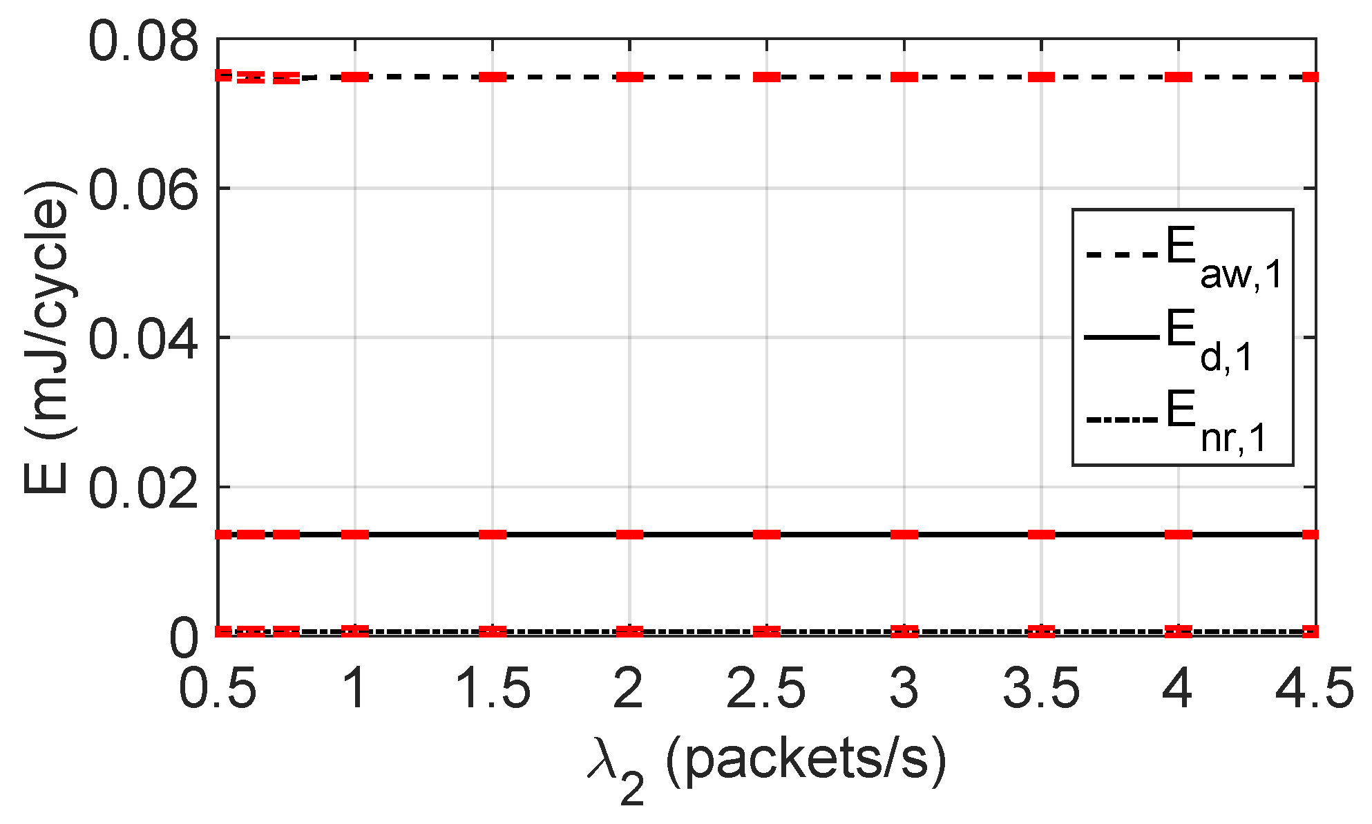
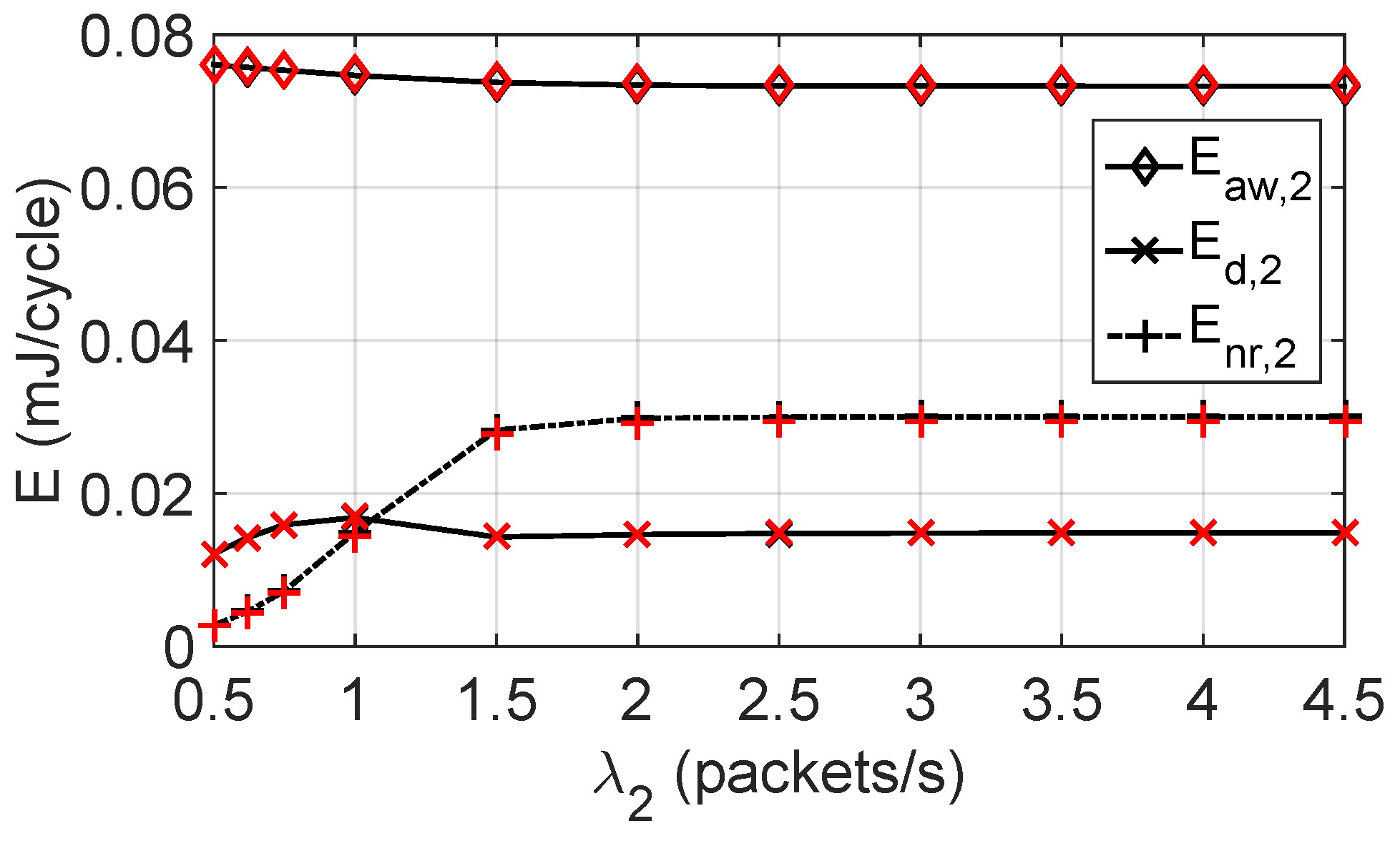
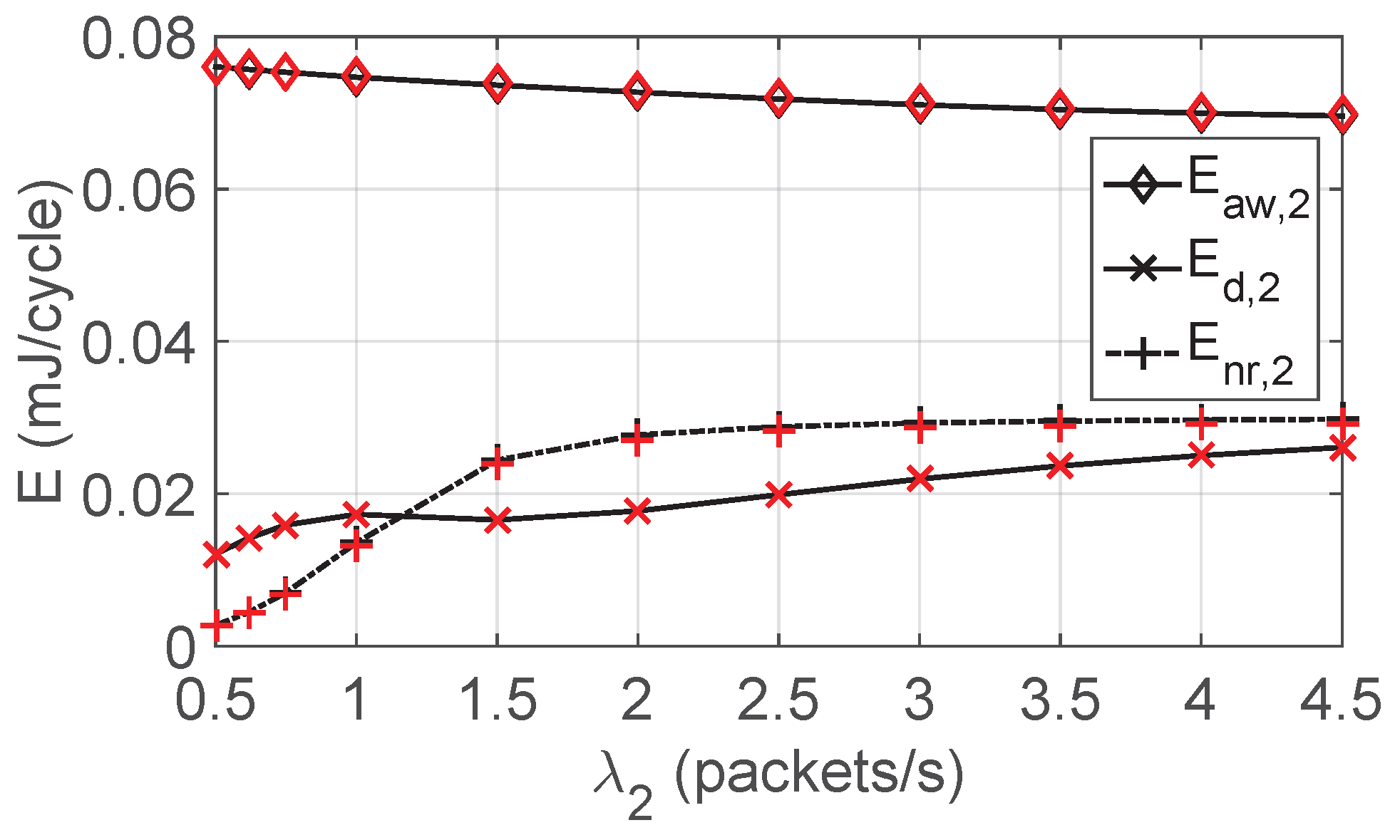
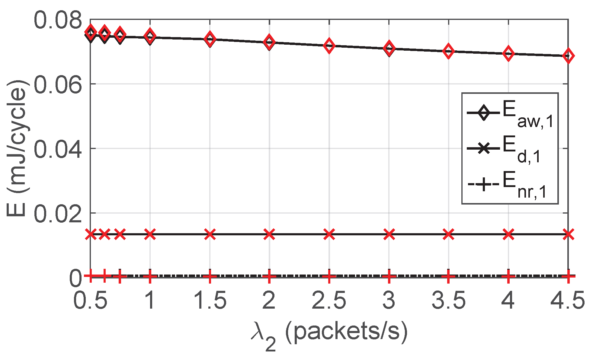
The proposed analytical model is an approximate model whose accuracy is validated by simulation. The analytical results have been obtained by solving the two 2D-DTMCs and finding their stationary probability distributions. On the other hand, simulation results have been obtained using a customized discrete-event simulation program developed in C language. It mimics the real behavior of the WSN. That is, in each cycle: (i) packets arrive in the queue of an SN according to a given discrete probability distribution; (ii) active SNs contend for channel access. (iii) if a SN wins the contention, it transmits a PF according to the transmission scheme configured in it (SPT or APT); (iv) if a collision occurs, all active SNs of the same class will switch to the sleep mode until the end of the cycle. The simulation results are completely independent from those obtained by the analytical model.

The simulation results presented have been obtained as the average of measurements performed over ${10}^8$ cycles. We have also obtained 95% confidence level intervals for the performance parameters of interest. However, being very small, they have been mostly omitted. For illustration purposes and as examples, confidence intervals have been drawn for the curves of Figure 3 and Figure 4. In the scenario studied in these figures, both classes deploy the SPT scheme ($F_1=F_2=1$), and the queue of $\mathrm{C}1$ and $\mathrm{C}2$ SNs can store a maximum of $Q_1=Q_2=10$ DATA packets, respectively. In these figures, black lines correspond to analytical values, while simulation values are represented by their corresponding red 95% confidence level intervals.

Please note that the load for $\mathrm{C}1$ SNs is constant (${\lambda }_1=0.5$ packets/s), while varies for $\mathrm{C}2$ SNs. The load offered to a single $\mathrm{C}1$ SN is one DATA packet every $33.3$ cycles, approximately, for a cycle of $T=60$ ms. The load offered to the 5 $\mathrm{C}1$ SNs is 5 DATA packets every $33.3$ cycles. On the other hand, when ${\lambda }_2=1$ packet/s, the load offered to a single $\mathrm{C}2$ SN is two DATA packet every $33.3$ cycles, approximately, and the load offered to the 20 $\mathrm{C}2$ SNs is 40 DATA packets every $33.3$ cycles.

Clearly, as ${\lambda }_2$ approaches 1 packet/s, the load offered to the WSN is larger than the maximum load the WSN can carry, i.e., $33.3$ DATA packet every $33.3$ cycles. As the offered load approaches the maximum carried load, the performance observed by $\mathrm{C}2$ SNs degrades, as $\mathrm{C}2$ SNs have lower access priority than $\mathrm{C}1$ SNs. Then, as observed in Figure 4, $\mathrm{C}2$ SNs experience a traffic congestion situation, even for traffic loads as small as ${\lambda }_2=0.5$ packet/s.

The energy consumed in awake cycles, $E_{aw,c}$, is identical for SNs of both classes. However, $E_{nr,2}$ is larger than $E_{nr,1}$. Recall that $E_{nr,c}$ measures the average energy consumed by $\mathrm{RN}c$ while it is in the sleep mode in normal cycles. Please note that $\mathrm{C}2$ SNs experience much more frequent collisions than $\mathrm{C}1$ SNs. Typically, an SN detects a collision when a CTS packet is not received after the transmission of the RTS packet. Upon detecting a collision, an SN switches to the sleep mode. Then, the time spent in the sleep mode is larger for classes that experience traffic congestion than for classes that do not experience it.

For the results presented in the following subsections, analytical results are represented by black lines with markers, while simulation results are represented by red markers. As it will be observed, the analytical and simulation markers completely overlap. This indicates a perfect match between the analytical and simulation results and proves that the results obtained by the approximate analytical model are very accurate.

5.3. Energy Consumed by $\mathrm{RN}1$ and $\mathrm{RN}2$ in the Data Period, the Awake and Normal Cycles

Figure 5 and Figure 6 show the energy consumed by $\mathrm{RN}1$ and $\mathrm{RN}2$ when deploying the APT transmission scheme with $F_1=F_2=2$ and $Q_1=Q_2=10$. Figure 5 shows that the energy consumed by $\mathrm{RN}1$ is virtually the same as in Figure 3, where $\mathrm{C}1$ SNs deployed the SPT scheme ($F_1=1$).

However, Figure 6 shows that $\mathrm{RN}2$ achieves the congestion state with a larger arrival rate than in the scenario of Figure 4, approximately, at an arrival rate twice as large as the previous one. In addition, the energy consumed in the congestion state is larger than the one consumed in the scenario of Figure 4, indicating that the packet throughput in the congestion state is larger when deploying $F_2=2$ (APT) than when deploying $F_2=1$ (SPT). The deployment of APT in $\mathrm{C}2$ SNs implies that more packets are sent when an SN wins the contention for medium access. This reduces the average number of active $\mathrm{C}2$ SNs per cycle, and, in turn, it leads to a higher medium access success rate.

Figure 7 and Figure 8 show the energy consumed by $\mathrm{RN}1$ and $\mathrm{RN}2$ when deploying the APT transmission scheme with $F_1=F_2=5$ and $Q_1=Q_2=10$. Also, Figure 9 and Figure 10 show the energy consumed by $\mathrm{RN}1$ and $\mathrm{RN}2$ when deploying the APT transmission scheme with $F_1=F_2=10$ and $Q_1=Q_2=10$.

As mentioned above, when large PFs are deployed ($F_c=5,10$), the average number of active nodes per cycle of a given class decreases with respect to scenarios with shorter PFs. This has a beneficial impact on the class, increasing its throughput and decreasing energy consumption, as fewer collisions occur and fewer retransmissions are required, which helps to conserve energy. Observe in Figure 7 that the energy consumed by $\mathrm{C}1$ SNs remain almost insensitive to the increase in the maximum PF size ($F_1$). However, for $\mathrm{C}2$ SNs, $E_{d,2}$ increases with the load, indicating that larger PFs are being transmitted when compared to the previous scenarios studied. Consequently, the $\mathrm{C}2$ SNs throughput is now also higher.

Note also the trend of the energy consumed in awake cycles as load increases. Clearly, $E_{aw,c}$ decreases as load increases, and this trend is more pronounced as the value of $F_c$ increases. This is because when an SN is in an awake cycle and transmits a PF with success, particularly when transmitting long PFs, it takes the SN longer to switch to the awake mode and activate the receiver. On the other hand, when an SN is in an awake cycle and transmits a PF that collides, the SN will switch to the awake operation mode and activate the receiver earlier than in cycles where the PF is successfully sent. Recall that a collision is detected quite early in the transmission process, when the corresponding CTS packet is not received. Then, the trend of the energy consumed in awake cycles as load increases clearly indicates that the success rate of transmitted PF increases with load as $F_c$ increases.

Note also that in the technical data sheet of the SN that has been used as a reference for the energy consumption values, the energy consumed in reception mode is larger than the one consumed while transmitting [29,31].

5.4. Energy Consumed by $\mathrm{RN}2$ Due to PF Transmissions with Success and Failure, and Due to Overhearing

In this subsection, we present the average energy consumed by $\mathrm{RN}1$ and $\mathrm{RN}2$ per cycle, along the data period of a cycle. We represent the variation of the different components of the energy consumed with the offered load to $\mathrm{C}2$ SNs (${\lambda }_2$), i.e., the energy consumed due to a PF transmitted with success, $E_{tx,s}^{d,2}$, the one when a PF collides, $E_{tx,f}^{d,2}$, and the one due to $\mathrm{RN}c$ overhearing the transmission of PFs by other SNs of the same class that win the contention to access the medium, $E_{oh}^{d,2}$. We also represent the total average energy consumed per cycle during the data period of a cycle, $E_{d,2}=E_{tx,s}^{d,2}+E_{tx,f}^{d,2}+E_{oh}^{d,2}$.

We evaluate a scenario where $\mathrm{C}c$ SNs deploy the APT transmission scheme with $F_1=F_2=10$ and have a queue capacity of $Q_1=Q_2=10$ DATA packets. The results are shown in Figure 11. Recall that $E_{oh}^{d,2}$ defines the average energy consumed by an active RN2 that looses the contention to access the channel. At the beginning of the data period of a cycle, active SNs start sensing the medium until their backoff timers expire or sense a busy medium. In the latter case, SNs move to the sleep mode until the end of the cycle. Then, $E_{oh}^{d,c}$ measures the average energy wasted by an active $\mathrm{RN}c$ per cycle due to having the receiver active to perform channel sensing along data periods where it loses the contention.

Observe that the average energy wasted per cycle due to PF collisions, $E_{tx,f}^{d,2}$, is almost negligible. That is, when $\mathrm{C}2$ SNs deploy the APT scheme with $F_2=10$, the packet collision rate is substantially reduced. As mentioned before, as F increases, fewer SNs per cycle are active, and a higher rate of successfully transmitted PFs is achieved.

To reinforce this perspective, we show the variation of the packet average access delay with the offered load to $\mathrm{C}2$ SNs (${\lambda }_2$), for different values of F in Figure 12. This figure is taken from [24]. Observe that the average DATA packet delay expressed in cycles for $\mathrm{C}1$ SNs, $D_1$, is insensitive to the value of $F_1$. However, $D_2$ decreases substantially as $F_2$ increases, confirming the benefits that can be obtained by deploying the APT scheme.

5.5. Accuracy of the New Methodology to Determine Energy Consumption

As mentioned in Section 1, the new proposed methodology to determine the average energy consumed by an SN per cycle has proved to be more accurate and systematic than those previously proposed. In this subsection, we compare the accuracy of the new methodology and the accuracy of a previous one [23] to determine the average energy consumed by an SN per cycle in the data period $E_{d,c}=E_{tx,s}^{d,c}+E_{tx,f}^{d,c}+E_{oh}^{d,c}$, $c=\left\{1,2\right\}$. Unfortunately, for the previous methodology, the average energy data consumed by an SN per cycle in the sleep mode and in awake cycles are not available.

A substantial part of the accuracy improvement of the new methodology with respect to previous ones [21,27,32,33,34] comes from the fact that previous energy computation methodologies required the definition of intermediate parameters, while in the new methodology, the energy computation is solely based on the stationary probability distribution ${\pi }_c\left(i,k\right)$, $c=\left\{1,2\right\}$.

As an example, Figure 13 shows the relative error of the average energy consumed by an SN per cycle in the data period in the scenario defined in Table 1. Relative values are obtained as $\left|x-y\right|/y$, where x is the value obtained by the analytical model, and y is the value obtained by simulation. Please note that ${\mathrm{P}}_{\mathrm{C}1}$ and ${\mathrm{P}}_{\mathrm{C}2}$ refer to the relative errors obtained using the previous methodology [23], while ${\mathrm{N}}_{\mathrm{C}1}$ and ${\mathrm{N}}_{\mathrm{C}2}$ refer to the relative errors obtained using the new methodology when measuring $E_{d,c}$, $c=\left\{1,2\right\}$, for $\mathrm{C}1$ and $\mathrm{C}2$ SNs, respectively.

Observe in Figure 13 that the relative errors represented for ${\mathrm{N}}_{\mathrm{C}1}$ and ${\mathrm{N}}_{\mathrm{C}2}$ are almost identical at each of the load points studied. Also, the relative errors represented for ${\mathrm{N}}_{\mathrm{C}1}$ and ${\mathrm{N}}_{\mathrm{C}2}$ have an homogeneous behavior with the load. Finally, we highlight that the relative errors of the new methodology are mostly below $1\%$, except for ${\lambda }_2=1$, where it is $1.5\%$,

However, the relative errors represented for ${\mathrm{P}}_{\mathrm{C}1}$ and ${\mathrm{P}}_{\mathrm{C}2}$ tend to have a less homogeneous behavior with the load than the relative errors obtained by the new methodology, and for ${\lambda }_2=1.5$, ${\mathrm{P}}_{\mathrm{C}2}$ achieves a relative error larger than $4.5\%$.

6. Conclusions

A novel energy consumption model has been proposed for sensor nodes that deploy the synchronous duty-cycled MAC protocol named Priority Sink Access MAC (PSA-MAC) in heterogeneous IoT WSNs. The new methodology to determine the average energy consumed by SNs in a cycle considers all the operation modes in the entire operation cycle. The model is based on two 2D-DTMCs that define the evolution of the active sensor nodes of each class, as well as the number of packets in their queues. Their stationary probability distributions are used to derive, in a systematic and conceptually simple way, closed-form expressions that allow to determine the average energy consumed by the sensor nodes along an operating cycle.

The model considers different classes of SNs, each with its own features and priority assignments, allowing the determination of the performance of complex heterogeneous WSNs. In addition, each class can independently support two packet transmission modes: the single DATA packet transmissions (SPT), or the more sophisticated aggregate DATA packet transmission (APT) mode.

The model has been designed to be able to compute the energy consumed in every period of the cycle, the sync (synchronization), data and sleep periods. In addition, the model considers normal and awake operating cycles. During a normal cycle, an inactive sensor node will remain in the sleep mode for the full duration of the cycle once the sync period ends. However, at the end of a sync period, active sensor nodes will start contending for access to the channel. After an active sensor node transmits a packet frame successfully, or as soon as it detects a collision, it will switch to the sleep mode. An active sensor node also switches to the sleep mode as soon as it detects that it has lost the contention. However, during awake cycles, an SN, instead of switching to the sleep mode, will remain awake until the end of the cycle to hear possible transmissions of SYNC packets. The proposed model determines the average energy consumed by an SN in both normal and awake cycles.

The accuracy of the proposed methodology to determine the average energy consumed by a sensor node in a cycle has been measured by comparing the results of the analytical model to those obtained by a customized discrete-event simulation program. The obtained results show that the approximate analytical model is very accurate.

In its current form, the model only considers ideal channels, i.e., an error-free channel from the MAC perspective. In a future work, we plan to extend the model to support a more realistic error-prone channel. This will allow the model to take into account the impact of the MAC layer, as well as the impact of the physical layer on the network performance.

References

1. Mansour, M.; Gamal, A.; Ahmed, A.I.; Said, L.A.; Elbaz, A.; Herencsar, N.; Soltan, A. Internet of Things: A Comprehensive Overview on Protocols, Architectures, Technologies, Simulation Tools, and Future Directions. Energies 2023, 16, 3465. [Google Scholar] [CrossRef]
2. Ahmed, S. Energy Aware Software Defined Network Model for Communication of Sensors Deployed in Precision Agriculture. Sensors 2023, 23, 5177. [Google Scholar] [CrossRef] [PubMed]
3. Pedditi, R.B.; Debasis, K. Energy Efficient Routing Protocol for an IoT-Based WSN System to Detect Forest Fires. Appl. Sci. 2023, 13, 3026. [Google Scholar] [CrossRef]
4. Chi, H.R.; Wu, C.K.; Huang, N.; Tsang, K.; Radwan, A. A Survey of Network Automation for Industrial Internet-of-Things Toward Industry 5.0. IEEE Trans. Ind. Inform. 2023, 19, 2065–2077. [Google Scholar] [CrossRef]
5. Li, B.; Zhao, Q.; Jiao, S.; Liu, X. DroidPerf: Profiling memory objects on android devices. In Proceedings of the 29th Annual International Conference on Mobile Computing and Networking (MobiCom 2023), Madrid, Spain, 2–6 October 2023; pp. 1–15. [Google Scholar]
6. Raut, S.; Bhandari, C.; Jain, H. A Comparative Study of Power Optimization Techniques for Microcontroller based IoT Applications. In Proceedings of the 2024 Fourth International Conference on Advances in Electrical, Computing, Communication and Sustainable Technologies (ICAECT), Bhilai, India, 11–12 January 2024; pp. 1–8. [Google Scholar]
7. Abdul-Qawy, A.; Alduais, N.; Saad, A.; Taher, M.; Nasser, A.; Saleh, S.; Khatri, N.B. An enhanced energy efficient protocol for large-scale IoT-based heterogeneous WSNs. Sci. Afr. 2023, 21, e01807. [Google Scholar] [CrossRef]
8. Abdulzahra, A.; Al-Qurabat, A.; Abdulzahra, S. Optimizing energy consumption in WSN-based IoT using unequal clustering and sleep scheduling methods. Internet Things 2023, 22, 100765. [Google Scholar] [CrossRef]
9. Banti, K.; Karampelia, I.; Dimakis, T.; Boulogeorgos, A.; Kyriakidis, T.; Louta, M. LoRaWAN Communication Protocols: A Comprehensive Survey under an Energy Efficiency Perspective. J. Telecom. 2022, 3, 322–357. [Google Scholar] [CrossRef]
10. Ghaderi, M.R.; Amiri, N. LoRaWAN sensor: Energy analysis and modeling. Wirel. Netw. 2024, 30, 1013–1036. [Google Scholar] [CrossRef]
11. Correia, F.; Alencar, M.; Assis, K. Stochastic Modeling and Analysis of the Energy Consumption of Wireless Sensor Networks. IEEE Lat. Am. Trans. 2023, 21, 434–440. [Google Scholar] [CrossRef]
12. Nguyen, M.T.; Nguyen, H.M.; Masaracchia, A.; Nguyen, C.V. Stochastic-Based Power Consumption Analysis for Data Transmission in Wireless Sensor Networks. EAI Endorsed Trans. Ind. Netw. Intell. Syst. 2019, 6, e5. [Google Scholar] [CrossRef]
13. Xu, D.; Wang, K. Stochastic Modeling and Analysis with Energy Optimization for Wireless Sensor Networks. Int. J. Distrib. Sens. Netw. 2014, 10, 672494. [Google Scholar] [CrossRef]
14. Rahimifar, A.; Kavian, Y.; Kaabi, H.; Soroosh, M. Predicting the energy consumption in software defined wireless sensor networks: A probabilistic Markov model approach. J. Ambient. Intell. Humaniz. Comput. 2021, 12, 9053–9066. [Google Scholar] [CrossRef]
15. Zhang, Y.; Li, W. Energy consumption analysis of a duty cycle wireless sensor network model. IEEE Access 2019, 7, 33405–33413. [Google Scholar] [CrossRef]
16. Xiao, W.; Kaneko, M.; El Rachkidy, N.; Guitton, A. Integrating lora collision decoding and mac protocols for enabling iot massive connectivity. IEEE Internet Things Mag. 2022, 5, 166–173. [Google Scholar] [CrossRef]
17. Wang, Y.; Vuran, M.C.; Goddard, S. Stochastic Analysis of Energy Consumption in Wireless Sensor Networks. In Proceedings of the 2010 7th Annual IEEE Communications Society Conference on Sensor, Mesh and Ad Hoc Communications and Networks (SECON), Boston, MA, USA, 21–25 June 2010; pp. 1–9. [Google Scholar]
18. Gallucio, L.; Palazzo, S. End-to-End Delay and Network Lifetime Analysis in a Wireless Sensor Network Performing Data Aggregation. In Proceedings of the 2010 In 2009 IEEE Global Telecommunications Conference (GLOBECOM 2009), Honolulu, HI, USA, 30 November–4 December 2010; pp. 1–6. [Google Scholar]
19. Li, Z.; Peng, Y.; Qiao, D.; Zhang, W. Joint Aggregation and MAC design to prolong sensor network lifetime. In Proceedings of the 2013 21st IEEE International Conference on Network Protocols (ICNP), Goettingen, Germany, 7–10 October 2013; pp. 1–10. [Google Scholar]
20. Li, Z.; Peng, Y.; Qiao, D.; Zhang, W. LBA: Lifetime balanced data aggregation in low duty cycle sensor networks. In Proceedings of the 31st Annual IEEE International Conference on Computer Communications (IEEE INFOCOM 2012), Orlando, FL, USA, 25–30 March 2012; pp. 1844–1852. [Google Scholar]
21. Guntupalli, L.; Martinez-Bauset, J.; Li, F.Y.; Weitnauer, A. Aggregated packet transmission in duty-cycled WSNs: Modeling and performance evaluation. IEEE Trans. Veh. Technol. 2016, 66, 563–579. [Google Scholar] [CrossRef]
22. Portillo, C.; Martinez-Bauset, J.; Pla, V.; Casares-Giner, V. Energy Modeling and Analysis for IoT Sensor Devices: A DTMC-Based Approach. In Proceedings of the Workshop on Innovation on Information and Communication Technologies (ITACA-WIICT 2018), Valencia, Spain, 13 July 2018; pp. 126–142. [Google Scholar]
23. Portillo, C.; Martinez-Bauset, J.; Pla, V.; Casares-Giner, V. Modeling of Duty-Cycled MAC Protocols for Heterogeneous WSN with Priorities. Electronics 2020, 9, 467. [Google Scholar] [CrossRef]
24. Portillo, C.; Martinez-Bauset, J.; Pla, V.; Casares-Giner, V. Heterogeneous WSN Modeling: Packet Transmission with Aggregation of Traffic. In Proceedings of the Interdisciplinary Conference on Mechanics, Computers and Electrics (ICMECE 2022), Barcelona, Spain, 6–7 October 2022; pp. 278–283. [Google Scholar]
25. Pereira, F.; Correia, R.; Carvalho, N.B. Comparison of active and passive sensors for IoT applications. In Proceedings of the 2018 IEEE Wireless Power Transfer Conference (WPTC), Montreal, QC, Canada, 3–7 June 2018; pp. 1–3. [Google Scholar]
26. Guntupalli, L.; Martinez-Bauset, J.; Li, F.Y. Performance of Frame Transmissions and Event-triggered Sleeping in Duty-Cycled WSNs with Error-Prone Wireless Links. Comput. Netw. 2018, 134, 215–227. [Google Scholar] [CrossRef]
27. Martinez-Bauset, J.; Guntupalli, L.; Li, F.Y. Performance analysis of synchronous duty-cycled MAC protocols. IEEE Wirel. Commun. Lett. 2015, 4, 469–472. [Google Scholar] [CrossRef]
28. Portillo, C.; Martinez-Bauset, J.; Pla, V.; Casares-Giner, V. The State Transition Probabilities of the Two 2D-DTMC with Traffic Aggregation. Technical Note. Available online: https://personales.upv.es/jmartine/public/2DDTMC.pdf (accessed on 10 June 2024).
29. MICAz Data Sheet. Crossbow Technology Incorporated, San Jose, CA, USA. Available online: http://courses.ece.ubc.ca/494/files/MICAz_Datasheet.pdf (accessed on 1 April 2024).
30. Zhang, S. Modeling, Analysis and Design of Energy Harvesting Communication Systems. Ph.D. Thesis, University of Rochester, Rochester, NY, USA, 2013. [Google Scholar]
31. Kramer, M.; Geraldy, A. Energy Measurements for Micaz Node; Technical Report KrGe06; University of Kaiserslautern: Kaiserslautern, Germany, 2006; pp. 1–6. [Google Scholar]
32. Yang, O.; Heinzelman, W. Modeling and throughput analysis for SMAC with a finite queue capacity. In Proceedings of the 2009 International Conference on Intelligent Sensors, Sensor Networks and Information Processing (ISSNIP), Melbourne, Australia, 7–10 December 2009; pp. 409–414. [Google Scholar]
33. Yang, O.; Heinzelman, W. Modeling and performance analysis for duty-cycled MAC protocols with applications to S-MAC and X-MAC. IEEE Trans. Mob. Comput. 2012, 11, 905–921. [Google Scholar] [CrossRef]
34. Portillo, C.; Martinez-Bauset, J.; Pla, V. Modelling of S-MAC for Heterogeneous WSN. In Proceedings of the 2018 9th IFIP International Conference on New Technologies, Mobility and Security (NTMS), Paris, France, 26–28 February 2018; pp. 1–6. [Google Scholar]
Figure 1. Heterogeneous WSN scenario with C 1 and C 1 SNs, and corresponding RN 1 and RN 2 .
Telecom 05 00036 g001
Figure 2. Transmission process in a transmission cycle for a heterogeneous WSN with two classes of nodes.
Telecom 05 00036 g002
Figure 3. Average energy consumed by RN 1 per cycle during the data period, and in the awake and normal cycles, when deploying SPT ( F 1 = 1 ).
Telecom 05 00036 g003
Figure 4. Average energy consumed by RN 2 per cycle during the data period, and in the awake and normal cycles, when deploying SPT ( F 2 = 1 ).
Telecom 05 00036 g004
Figure 5. Average energy consumed by RN 1 per cycle during the data period, and in the awake and normal cycles, when deploying APT ( F 1 = 2 ).
Telecom 05 00036 g005
Figure 6. Average energy consumed by RN 2 per cycle during the data period, and in the awake and normal cycles, when deploying APT ( F 2 = 2 ).
Telecom 05 00036 g006
Figure 7. Average energy consumed by RN 1 per cycle during the data period, and in the awake and normal cycles, when deploying APT ( F 1 = 5 ).
Telecom 05 00036 g007
Figure 8. Average energy consumed by RN 2 per cycle during the data period, and in the awake and normal cycles, when deploying APT ( F 2 = 5 ).
Telecom 05 00036 g008
Figure 9. Average energy consumed by RN 1 per cycle during the data period, and in the awake and normal cycles, when deploying APT ( F 1 = 10 ).
Telecom 05 00036 g009
Figure 10. Average energy consumed by RN 2 per cycle during the data period, and in the awake and normal cycles, when deploying APT ( F 2 = 10 ).
Telecom 05 00036 g010
Figure 11. Average energy consumed by RN 2 per cycle due to PF transmissions with success and failure, and to overhearing, when deploying APT ( F 2 = 10 ).
Telecom 05 00036 g011
Figure 12. Average packet delay for both SNs classes.
Telecom 05 00036 g012
Figure 13. Average relative errors of the current and previous (Pre-method) energy computation methodologies.
Telecom 05 00036 g013