Imaging, Dynamic Histomorphometry, and Mechanical Testing in Preclinical Bone Research


Department of Biomedicine, Aarhus University, 8000 Aarhus, Denmark
Osteology 2024, 4(3), 120-131; https://doi.org/10.3390/osteology4030010 (registering DOI)
Submission received: 25 May 2024
/
Revised: 12 July 2024
/
Accepted: 18 July 2024
/
Published: 24 July 2024
Abstract
:Advanced laboratory methods play a crucial role in bone research, allowing researchers and scientists to study the complex biology and nature of the skeleton. Dual-energy X-ray absorptiometry (DXA) is a non-invasive method of measuring bone mass, which is an important parameter for the diagnosis and treatment of several bone diseases. Micro-computed tomography (μCT) is a very high-resolution technique that can be used to investigate the 3D microstructure of trabecular bone. Dynamic bone histomorphometry is used to assess histological indices of bone formation and resorption using fluorochromes embedded into newly formed bone. Mechanical testing is used to measure bone strength and stiffness, providing important information about bone quality and fracture risk. All these methods are widely used in preclinical in vivo studies using rodents and in most clinical studies. Therefore, it is important for both researchers and scientists within the field of bone biology, and those in neighboring fields, to be familiar with their use, strengths, limitations, and important technical aspects. Several guidelines and protocols about the topic have been published, but are very exhaustive. The present review aimed to provide instructions for early-career researchers and outline important concepts and technical aspects of DXA, μCT, dynamic bone histomorphometry, and mechanical testing in bone research.
1. Introduction
Bone research is a multidisciplinary field of study that focuses on structure, function, skeletal development, and bone cells, as well as prevention and treatment strategies for bone-related diseases such as osteoporosis. The field is complex, rapidly evolving, and requires in-depth background knowledge about the use of advanced laboratory techniques, and this can be overwhelming for researchers and scientists outside the field of skeletal research.
In 1994, the World Health Organization (WHO) published revised diagnostic criteria for osteoporosis in post-menopausal women that for the first time included the use of dual-energy X-ray absorptiometry (DXA) to assess bone mass [1]. These criteria (T-score ≤ −2.5) have been widely accepted and are used in clinical medicine to provide intervention thresholds for treatment and as inclusion criteria in clinical trials of new pharmaceutical countermeasures [2]. In contrast to clinical medicine, preclinical skeletal biomedicine studies in rodents have embraced the use of micro-computed tomography (μCT) to study delicate microstructural parameters and asses the true 3D nature of bone. Similarly, dynamic bone histomorphometry and destructive mechanical testing of bone samples are extensively used in preclinical research.
The present review aimed to briefly and conveniently introduce the use of DXA to assess areal bone mineral density (aBMD) and bone mineral content (BMC), μCT to assess 3D trabecular microstructure and cortical morphology, dynamic bone histomorphometry to assess various histological indices of bone formation and resorption, and destructive mechanical testing to assess maximum bone strength. All these methods are widely used in skeletal research and are among the most used investigative methods in preclinical in vivo studies of skeletal deterioration from disuse in rodents [3,4]. Moreover, guidelines and statement papers are referenced and highlighted to easily redirect readers to more in-depth and detailed resources that are available elsewhere.
2. Dual-Energy X-ray Absorptiometry (DXA)
Bone mineral density can be measured using DXA because soft tissue and bone have different attenuation coefficients to X-rays [5,6]. Two X-rays with different energy levels are emitted from a radiation source aimed at the sample placed in front of a radiation detector. It is not possible to determine the amount of attenuation attributed to bone alone from a single X-ray passing through the sample [7]. Measurement of the transmission factors at two distinct energies allows the areal densities (i.e., mass per unit of projected area) of two different types of tissue (hydroxyapatite as bone mineral and soft tissue) to be deduced because the X-ray attenuation coefficient depends on both atomic number and photon energy. Hence, when two X-rays are used, the attenuation from soft tissue can be subtracted from the total absorption, leaving the attenuation attributed to bone and vice versa [5]. The DXA system is connected to a computer for analysis, where the raw data are processed to produce a map of aBMD that is computed pixel by pixel over the whole scan area and provides an image of the bone mineral density distribution (Figure 1) [5,6].
Since DXA uses 2D projections of the total distribution of BMC, it does not allow for a direct portrait of the 3D structure of bone. The 2D nature of DXA warrants careful and identical placement of bone samples when performing multiple scans since differences in bone area will substantially affect the calculation of aBMD. However, DXA is relatively simple to use, results are rapidly obtained, and the specimen is only exposed to low radiation compared to μCT for the quantitative analysis of changes in bone [8].
Figure 1.
DXA of the whole femur of rats injected with saline (Ctrl) or botulinum toxin type A (BTX). Purple color represents low bone mineral density and yellow color represents high bone mineral density. Note how the femoral bone mineral density is noticeably lower in the BTX-injected immobilized hind limb compared with Ctrl. Adapted from [9].

Newer DXA systems can compute a trabecular bone score (TBS) calculated from 2D projection images [10]. TBS has been evaluated in ex vivo studies of human cadaveric vertebrae for correlation analyses with trabecular microstructure obtained by μCT (maximum r2 = 0.67 for connectivity density) [11]. Instead, μCT can be used to measure 3D bone microstructure directly. Another limitation of DXA is that it might underestimate aBMD if excessive soft tissue is present on the bone samples, and fat tissue is also a major constraint on the accuracy [12]. Adipose tissue differs from lean tissue in its X-ray attenuation coefficient due to its higher hydrogen content. Variations in the soft tissue composition along the X-ray beam’s path through bone when compared to the nearby soft tissue reference area can therefore result in errors in the aBMD measurements. Therefore, soft tissue must carefully be removed from all bones before DXA scanning to minimize inaccurate estimations [5]. Finally, it is important to regularly perform quality assurance of the DXA scanner according to the manufacturer’s guidelines to ensure valid results.
No complete standardized protocol or guideline exists for the use of DXA in preclinical biomedicine research. However, Shi et al. published a guideline for the use of DXA to analyze trabecular bone-rich regions in mice [13]. They compared the correlation between BMC estimates from DXA with those obtained from micro-computed tomography (μCT) and found a strong correlation for the distal femur and proximal tibia (r = 0.85 and r = 0.88), respectively.
For the use of DXA in a clinical setting, Lewieck et al. published best practice guidelines to ensure high-quality acquisition, analysis, or interpretation of DXA data [14].
3. Micro-Computed Tomography (μCT)
The first μCT system was conceived in the early 1980s [15] and was first used to examine the 3D architecture of bone in 1989 [16]. The method allows for an extremely detailed investigation of cortical morphology and trabecular microstructure (Figure 2). The μCT system utilizes X-rays that travel through the bone sample to record a 2D projection on a detector placed behind the sample. The sample is rotated on a rotational stage in order to produce projections from all angles. Specialized computer software is then used to reconstruct a 3D volume from all the 2D projection images [17].
Since the attenuation of X-rays is dependent on atomic number, tissues with different X-ray attenuation can be separated [19]. However, attenuation is most pronounced where the bone sample is most dense and thickest because photons with higher energies are required to penetrate denser and thicker bone. Consequently, beam hardening effects might arise because only high-energy photons are left to contribute to the mean X-ray beam energy level. However, beam hardening effects can be reduced by placing a 0.5 mm aluminum filter between the micro-focus X-ray tube and the bone sample to narrow the photon energy spectrum.
It is essential to carefully consider the optimal voxel size to use for μCT scanning. Density artifacts can materialize if μCT scans are conducted using inappropriately large voxels. Volumetric bone mineral density (vBMD) might be underestimated due to the partial volume effect, and the object thickness is overestimated if a voxel size that is too large is used [17,20]. Moreover, if a voxel size that is too large is used relative to the microstructure of interest, the μCT scans will appear blurry, and delicate details might be lost (Figure 3). This effect is even more pronounced after lowpass filtration and segmentation.
One might argue that the smallest possible voxel size should always be used; however, this will inevitably result in larger data sets, more wear on the X-ray tube, and longer acquisition times. In theory, the Nyquist sampling theorem states that the sampling distance must be less than half the desired resolution distance. In practice, the manufacturer of the μCT system usually recommends using a voxel size not only two times smaller but also at least six times smaller than the size of the structure of interest (Scanco Medical, Wangen-Brüttisellen, Switzerland) [22]. Therefore, the desired voxel size used must be chosen carefully to ensure an optimal trade-off between scan time and voxel size.
The information content of a voxel depends on the sensitivity of the charge-coupled device detector and the signal-to-noise ratio (SNR). The total number of photons for each projection is dependent on the integration time, tube current, and number of times each projection is repeated (frame-averaged). The SNR can be improved by increasing the frame averaging and integration time, but this comes with a trade-off of higher radiation exposure and longer scan times (Figure 4) [17].
Another potential source of error is the incorrect delineation of volumes of interest (VOIs) to separate trabecular and cortical bone. For VOIs including trabecular bone, contours may be drawn manually a few voxels away from the endocortical surface and semi-automatically morphed across slices. The slices should then be visually inspected to ensure that the semi-automatic morphing contours have not drifted to include cortical bone. Other options include irregular anatomical contouring at the edge of the endocortical bone surface or a regular, uniformly shaped VOI, such as a cylinder or circle, delineated within the trabecular network (Figure 5).
Several guidelines and protocols for the use of μCT to assess rodent bone or dentoalveolar microstructure in biomedicine research have been published [17,20,23,24]. Nevertheless, the authoritative Journal of Bone and Mineral Research (JBMR) guideline by Bouxsein et al. should be followed to ensure consistency and standardized terminology when reporting results from in vivo μCT studies in rodents [17]. Table 1 is an adapted and short version of the minimum required reporting for such studies, μCT scan acquisition, and outcomes for trabecular bone microstructure and cortical morphology. The complete reporting guideline is available elsewhere [17].
4. Dynamic Bone Histomorphometry
The foundation for dynamic bone histomorphometry was established in 1957, when it was discovered that tetracycline is deposited in vivo into bone and that its fluorescence can be studied in undecalcified sections [25]. Later, Harold Frost (1921–2004) [26,27] and others [28,29] developed and refined different approaches to study histological bone remodeling using fluorescence microscopy. Since the initial studies with tetracycline, several other fluorochromes have been used successfully to label bone, such as alizarin, calcein green and blue, xylenol orange, doxycycline, and rolitetracycline (Figure 5) [30,31]. Today, dynamic bone histomorphometry is widely used by both basic scientists and clinicians.
The method is commonly used to assess mineralizing surface (MS/BS), mineral apposition rate (MAR), and bone formation rate (BFR/BS). To quantify the number of intersections with bone surfaces and the presence of single or double fluorochrome labels, an unbiased 2D counting frame and a randomly orientated line grid can be superimposed on the field of view, as demonstrated by Vegger et al. [32]. MS/BS denotes the amount of bone surface undergoing active mineralization and is calculated as the number of intersections with double fluorochrome labels plus half the number of intersections with single labels divided by the total number of intersections with an intact bone surface. MAR provides information about the average amount of bone mineral apposition and is calculated as the distance between the midpoints of two consecutive fluorochrome labels divided by the inter-labeling period. BFR/BS is the bone formation rate per unit of bone surface and is calculated as MS/BS × MAR [33].
If two fluorochromes are injected sequentially to generate double labels, it is important to inject them an appropriate number of days apart to be able to distinguish their individual fluorescence correctly. An inter-labeling period of 4 or 7 days can be used for mice and rats, respectively. When using double fluorochrome labels, there is also an inherent risk of “label escape” where only one fluorochrome label is present because formation either began after the first label was given or stopped before the second was given [34].
The visualization of fluorescent bone labels can be complicated by the pale green autofluorescence that calcified bone emits under ultraviolet light (Figure 6).
However, this can be overcome by increasing the camera exposure time or using fluorochromes in sharp contrast to pale green. Alternatively, narrow bandpass filters can be used. Tetracycline (yellow), alizarin (red), and calcein (green) were used in the experiment depicted in Figure 6, and these fluorochromes are relatively easy to distinguish from the pale green autofluorescence emitted by calcified bone. Alternatively, a red HC-mFISH filter (AHF Analysentechnik, Tübingen, Germany) for alizarin labels and a BV-2A filter (Nikon, Tokyo, Japan) for calcein labels can be used as needed to more easily distinguish these bone-specific fluorochromes. Similarly, other filters exist for fluorochromes with different emittance spectrums.
Dynamic bone histomorphometry is very labor-intensive and repetitive and is thus an attractive target for computational optimization using artificial intelligence (AI). The use of AI in bone research is rapidly evolving and has recently been reviewed in detail elsewhere [36].
The authoritative guideline on the standardized nomenclature system for bone histomorphometry, including static and dynamic parameters, was updated in 2012 by the ASMBR Histomorphometry Nomenclature Committee [33].
5. Mechanical Testing
The mechanical behavior of bone is determined by its geometrical shape and the properties of the material that it consists of [37]. The geometrical shapes of bones are very heterogeneous. Long bones comprise a large diaphysis, which almost exclusively contains cortical bone, and a smaller and wider portion towards the joints called the metaphysis, with a rich trabecular network. In contrast, irregular bones such as vertebrae mainly comprise a dense trabecular network surrounded by a thin layer of cortical bone [38].
Bone is a prime example of a material with spatial gradients in composition and structure. The material of bone consists of minerals, hydroxyapatite, the framework protein type I collagen (>90% of the organic component of bone), many other so-called non-collagenous proteins, and water [39]. Bone tissue exhibits a hierarchical structure that varies over various length scales (hierarchical structure in decreasing size: whole bone; compact and trabecular bone; osteonal and circumferential lamellar bone; structural organization of fibers into parallel arrays; woven, lamellar, or root dentin structures; mineralized collagen fibril arrays; mineralized collagen fibrils; collagen fibrils; and crystals) [37]. It is also a graded material as it may differ from one place to another either continuously or in distinct stages in terms of its composition, structure, and mechanical qualities. Because of the combination of these two characteristics, a material type is created that is extremely complex and cannot be adequately characterized by a single material property value.
Bending tests are by far the most common methods used to test whole bones; they are particularly used to characterize the mechanical behavior of small experimental animals such as mice and rats. Most investigations of the mechanical performance of whole bones from preclinical animal studies are conducted using 3-point bending tests. However, torsional loading and impact loading are also used, though less frequently [40].
For the 3-point bending test, when vertical load is applied to the mid-diaphysis of a long bone, one side of the bone undergoes tension, while the other side is loaded in compression (Figure 7) [37]. Fractures originate from the tension side and then progress to the compression side where the load is applied because bones are stronger in compression than in tension [41]. Long bones bear some resemblance to a tube, for which resistance towards bending is directly related to material stiffness and the moment of inertia. The cross-sectional moment of inertia (I) of a tube depends on the inner radius (ri) and outer radius (ro) and is given as follows [37]:
Consequently, small increases in the outer radius will substantially increase the moment of inertia and thus the bone strength.
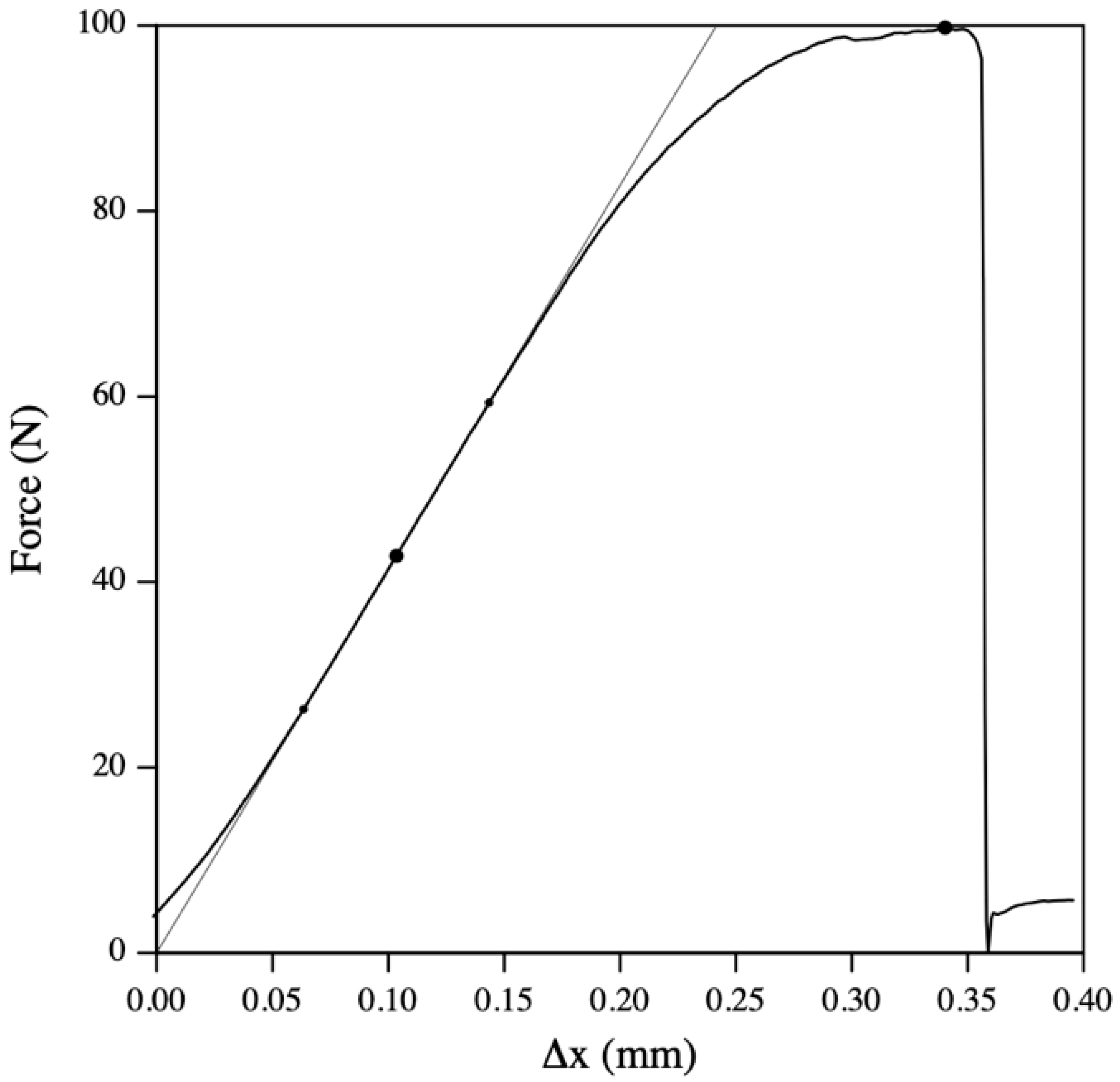
The maximum load to failure is determined as the highest force achieved at any point during compression testing (Figure 8). Load and deformation are linearly proportional until the yield point is reached. When the yield point is exceeded, the slope of the curve will start to decrease, and the bone will undergo plastic deformation that renders the bone unable to return to its original shape after unloading [42]. The plastic deformation results in irreversible structural damage such as slippage of cement lines, microcracks, and nanoscale damage of crystals and molecular arrangement. In contrast, elastic deformation occurs until the yield point, where the bone can elastically return most of the energy required for deformation and return to its original structure and shape [37,42].
The process of torsion testing a whole bone involves firmly embedding the tested epiphyseal ends in rectangular or cylindrical plastic material blocks that are fitted into the grips of the torsion testing machine [44,45]. This allows an approximate determination of the shear modulus of bone. One of several testing devices is used to apply a torque (twisting moment) to one of these grips while the other is kept firm. The load and angular deformation are then recorded [46]. In contrast, predicting how bones will behave under sudden loads in non-physiological directions (such as falling or high-velocity impact) requires simulating trauma-associated loading conditions, which demands high strain rates [47]. This fact prompted the development of a class of impact-type loading devices, such as pendulum loading, which involves dropping a precisely known-weight hammer from a known height (so that its potential energy is known) and hitting the bone sample with it. The results of these experiments can be used to determine how resistant whole bones are to impact loading at different configurations [41].
Destructive mechanical testing is the “gold standard” for determining bone strength and is an invaluable tool in preclinical research, but the method has some important inherent limitations. Mechanical testing results in the destruction of the bone sample, which renders it impossible to repeat the test if necessary. However, finite element models based on 3D data obtained with µCT can use the skeletal microstructure to predict bone strength non-destructively. Studies have shown that 80–90% of the variance in mechanical bone strength can be predicted by the finite element analysis estimate (vertebra: r2 = 0.78, proximal femur: r2 = 0.82, and distal radius: r2 = 0.92), and the method has been validated in both rodent and human bone samples [48]. Another limitation of mechanical testing is the inability to determine the relative contribution of bone density, material properties, and morphology to bone strength, and the method is unsuitable for clinical studies in humans. Finally, bone samples should be stored fresh-frozen for mechanical testing since storage in formalin or alcohol fixation changes the plastic mechanical properties of bone [49].
No authoritative guideline for mechanical testing exists for in vivo studies using rodents. However, several exhaustive reviews and protocol articles with illustrious figures have emerged, and readers are kindly referred to these for a more in-depth explanation of the mechanical testing of bones in biomedical science [9,37,42,50].
6. Conclusions
In vivo biomedical research uses a wide variety of advanced laboratory methods to investigate skeletal biology. Frequently used methods, such as DXA, μCT, dynamic histomorphometry, and mechanical testing are important to be familiar with for researchers and scientists conducting preclinical and translational bone research. The present review offers a concise introduction and richly illustrated brief overview of these methods and discusses their strengths, limitations, and technical nuances.
Funding
This research received no external funding.
Acknowledgments
The author is thankful for the unwavering support, academic mentorship, and invaluable insights about bone biology and laboratory methods that were instrumental in shaping the present review from Annemarie Brüel and Jesper Skovhus Thomsen. The present review is part of the author’s higher doctoral dissertation.
Conflicts of Interest
The author declares no conflicts of interest.
References
- Kanis, J.A.; Melton, L.J.; Christiansen, C.; Johnston, C.C.; Khaltaev, N. The Diagnosis of Osteoporosis. J. Bone Miner. Res. 1994, 9, 1137–1141. [Google Scholar] [CrossRef] [PubMed]
- Kanis, J.A.; McCloskey, E.V.; Johansson, H.; Oden, A.; Melton, L.J.; Khaltaev, N. A Reference Standard for the Description of Osteoporosis. Bone 2008, 42, 467–475. [Google Scholar] [CrossRef] [PubMed]
- Brent, M.B.; Brüel, A.; Thomsen, J.S. A Systematic Review of Animal Models of Disuse-Induced Bone Loss. Calcif. Tissue Int. 2021, 108, 561–575. [Google Scholar] [CrossRef] [PubMed]
- Donnelly, E. Methods for Assessing Bone Quality: A Review. Clin. Orthop. Relat. Res. 2011, 469, 2128. [Google Scholar] [CrossRef] [PubMed]
- Blake, G.M.; Fogelman, I. Technical Principles of Dual Energy X-Ray Absorptiometry. Semin. Nucl. Med. 1997, 27, 210–228. [Google Scholar] [CrossRef] [PubMed]
- Cullum, I.D.; Ell, P.J.; Ryder, J.P. X-Ray Dual-Photon Absorptiometry: A New Method for the Measurement of Bone Density. Br. J. Radiol. 1989, 62, 587–592. [Google Scholar] [CrossRef] [PubMed]
- Cherian, K.E.; Kapoor, N.; Meeta, M.; Paul, T.V. Dual-Energy X-Ray Absorptiometry Scanning in Practice, Technical Aspects, and Precision Testing. J. Midlife Health 2021, 12, 252. [Google Scholar] [CrossRef] [PubMed]
- Messina, C.; Maffi, G.; Vitale, J.A.; Ulivieri, F.M.; Guglielmi, G.; Sconfenza, L.M. Diagnostic Imaging of Osteoporosis and Sarcopenia: A Narrative Review. Quant. Imaging Med. Surg. 2018, 8, 86–99. [Google Scholar] [CrossRef]
- Brent, M.B.; Lodberg, A.; Thomsen, J.S.; Brüel, A. Rodent Model of Disuse-Induced Bone Loss by Hind Limb Injection with Botulinum Toxin A. MethodsX 2020, 7, 101079. [Google Scholar] [CrossRef]
- Martineau, P.; Leslie, W.D. Trabecular Bone Score (TBS): Method and Applications. Bone 2017, 104, 66–72. [Google Scholar] [CrossRef]
- Hans, D.; Barthe, N.; Boutroy, S.; Pothuaud, L.; Winzenrieth, R.; Krieg, M.A. Correlations Between Trabecular Bone Score, Measured Using Anteroposterior Dual-Energy X-Ray Absorptiometry Acquisition, and 3-Dimensional Parameters of Bone Microarchitecture: An Experimental Study on Human Cadaver Vertebrae. J. Clin. Densitom. 2011, 14, 302–312. [Google Scholar] [CrossRef] [PubMed]
- Cherif, R.; Vico, L.; Laroche, N.; Sakly, M.; Attia, N.; Lavet, C. Dual-Energy X-Ray Absorptiometry Underestimates in Vivo Lumbar Spine Bone Mineral Density in Overweight Rats. J. Bone Miner. Metab. 2018, 36, 31–39. [Google Scholar] [CrossRef] [PubMed]
- Shi, J.; Lee, S.; Uyeda, M.; Tanjaya, J.; Kim, J.K.; Pan, H.C.; Reese, P.; Stodieck, L.; Lin, A.; Ting, K.; et al. Guidelines for Dual Energy X-Ray Absorptiometry Analysis of Trabecular Bone-Rich Regions in Mice: Improved Precision, Accuracy, and Sensitivity for Assessing Longitudinal Bone Changes. Tissue Eng. Part C Methods 2016, 22, 451–463. [Google Scholar] [CrossRef] [PubMed]
- Lewiecki, E.M.; Binkley, N.; Morgan, S.L.; Shuhart, C.R.; Camargos, B.M.; Carey, J.J.; Gordon, C.M.; Jankowski, L.G.; Lee, J.K.; Leslie, W.D. Best Practices for Dual-Energy X-Ray Absorptiometry Measurement and Reporting: International Society for Clinical Densitometry Guidance. J. Clin. Densitom. 2016, 19, 127–140. [Google Scholar] [CrossRef] [PubMed]
- Elliott, J.C.; Dover, S.D. X-ray Microtomography. J. Microsc. 1982, 126, 211–213. [Google Scholar] [CrossRef] [PubMed]
- Feldkamp, L.A.; Goldstein, S.A.; Parfitt, M.A.; Jesion, G.; Kleerekoper, M. The Direct Examination of Three-dimensional Bone Architecture in Vitro by Computed Tomography. J. Bone Miner. Res. 1989, 4, 3–11. [Google Scholar] [CrossRef]
- Bouxsein, M.L.; Boyd, S.K.; Christiansen, B.A.; Guldberg, R.E.; Jepsen, K.J.; Müller, R. Guidelines for Assessment of Bone Microstructure in Rodents Using Micro-Computed Tomography. J. Bone Miner. Res. 2010, 25, 1468–1486. [Google Scholar] [CrossRef] [PubMed]
- Brent, M.B.; Thomsen, J.S.; Brüel, A. Short-Term Glucocorticoid Excess Blunts Abaloparatide-Induced Increase in Femoral Bone Mass and Strength in Mice. Sci. Rep. 2021, 11, 12258. [Google Scholar] [CrossRef] [PubMed]
- Shivaramu Effective Atomic Numbers for Photon Energy Absorption and Photon Attenuation of Tissues from Human Organs. Med. Dosim. 2002, 27, 1–9. [CrossRef]
- Christiansen, B.A. Effect of Micro-Computed Tomography Voxel Size and Segmentation Method on Trabecular Bone Microstructure Measures in Mice. Bone Rep. 2016, 5, 136–140. [Google Scholar] [CrossRef]
- Brent, M.B.; Simonsen, U.; Thomsen, J.S.; Brüel, A. Effect of Acetazolamide and Zoledronate on Simulated High Altitude-Induced Bone Loss. Front. Endocrinol. 2022, 13, 831369. [Google Scholar] [CrossRef] [PubMed]
- Zhao, Z.; Gang, G.J.; Siewerdsen, J.H. Noise, Sampling, and the Number of Projections in Cone-Beam CT with a Flat-Panel Detector. Med. Phys. 2014, 41, 061909. [Google Scholar] [CrossRef]
- du Plessis, A.; Broeckhoven, C.; Guelpa, A.; le Roux, S.G. Laboratory X-Ray Micro-Computed Tomography: A User Guideline for Biological Samples. Gigascience 2017, 6, gix027. [Google Scholar] [CrossRef] [PubMed]
- Chavez, M.B.; Chu, E.Y.; Kram, V.; de Castro, L.F.; Somerman, M.J.; Foster, B.L. Guidelines for Micro–Computed Tomography Analysis of Rodent Dentoalveolar Tissues. JBMR Plus 2021, 5, e10474. [Google Scholar] [CrossRef]
- Milch, R.A.; Rall, D.P.; Tobie, J.E. Bone Localization of the Tetracyclines. J. Natl. Cancer Inst. 1957, 19, 87–93. [Google Scholar] [CrossRef]
- Frost, H.M. Tetracycline-Based Histological Analysis of Bone Remodeling. Calcif. Tissue Res. 1969, 3, 211–237. [Google Scholar] [CrossRef] [PubMed]
- Frost, H.M. Measurement of Human Bone Formation By Means of Tetracycline Labelling. Can. J. Biochem. Physiol. 1963, 41, 31–42. [Google Scholar] [CrossRef] [PubMed]
- Marotti, G.; Marotti, F. Topographic-Quantitative Study of Bone Tissue Formation and Reconstruction in Inert Bones. In Calcified Tissues 1965; Springer: Berlin/Heidelberg, Germany, 1966; pp. 89–93. [Google Scholar]
- Haas, H.G.; Müller, J.; Schenk, R.K. Osteomalacia: Metabolic and Quantitative Histologic Studies. Clin. Orthop. Relat. Res. 1967, 53, 213–222. [Google Scholar] [CrossRef]
- van Gaalen, S.M.; Kruyt, M.C.; Geuze, R.E.; de Bruijn, J.D.; Alblas, J.; Dhert, W.J.A. Use of Fluorochrome Labels in in Vivo Bone Tissue Engineering Research. Tissue Eng. Part B Rev. 2010, 16, 209–217. [Google Scholar] [CrossRef]
- Pautke, C.; Vogt, S.; Tischer, T.; Wexel, G.; Deppe, H.; Milz, S.; Schieker, M.; Kolk, A. Polychrome Labeling of Bone with Seven Different Fluorochromes: Enhancing Fluorochrome Discrimination by Spectral Image Analysis. Bone 2005, 37, 441–445. [Google Scholar] [CrossRef]
- Vegger, J.B.; Brüel, A.; Dahlgaard, A.F.; Thomsen, J.S. Alterations in Gene Expression Precede Sarcopenia and Osteopenia in Botulinum Toxin Immobilized Mice. J. Musculoskelet. Neuronal Interact. 2016, 16, 355–368. [Google Scholar] [PubMed]
- Dempster, D.W.; Compston, J.E.; Drezner, M.K.; Glorieux, F.H.; Kanis, J.A.; Malluche, H.; Meunier, P.J.; Ott, S.M.; Recker, R.R.; Parfitt, A.M. Standardized Nomenclature, Symbols, and Units for Bone Histomorphometry: A 2012 Update of the Report of the ASBMR Histomorphometry Nomenclature Committee. J. Bone Miner. Res. 2013, 28, 2–17. [Google Scholar] [CrossRef] [PubMed]
- Schwartz, M.P.; Recker, R.R. The Label Escape Error: Determination of the Active Bone-Forming Surface in Histologic Sections of Bone Measured by Tetracycline Double Labels. Metab. Bone Dis. Relat. Res. 1982, 4, 237–241. [Google Scholar] [CrossRef] [PubMed]
- Brent, M.B.; Brüel, A.; Thomsen, J.S. PTH (1–34) and Growth Hormone in Prevention of Disuse Osteopenia and Sarcopenia in Rats. Bone 2018, 110, 244–253. [Google Scholar] [CrossRef] [PubMed]
- Brent, M.B.; Emmanuel, T. Contemporary Advances in Computer-Assisted Bone Histomorphometry and Identification of Bone Cells in Culture. Calcif. Tissue Int. 2023, 112, 1–12. [Google Scholar] [CrossRef] [PubMed]
- Sharir, A.; Barak, M.M.; Shahar, R. Whole Bone Mechanics and Mechanical Testing. Vet. J. 2008, 177, 8–17. [Google Scholar] [CrossRef] [PubMed]
- Clarke, B. Normal Bone Anatomy and Physiology. Clin. J. Am. Soc. Nephrol. 2008, 3 (Suppl. S3), S131. [Google Scholar] [CrossRef] [PubMed]
- Von Euw, S.; Wang, Y.; Laurent, G.; Drouet, C.; Babonneau, F.; Nassif, N.; Azaïs, T. Bone Mineral: New Insights into Its Chemical Composition. Sci. Rep. 2019, 9, 8456. [Google Scholar] [CrossRef]
- Simkin, A.; Robin, G. The Mechanical Testing of Bone in Bending. J. Biomech. 1973, 6, 31–39. [Google Scholar] [CrossRef]
- Turner, C.H. Bone Strength: Current Concepts. In Proceedings of the Annals of the New York Academy of Sciences; Blackwell Publishing Inc.: Hoboken, NJ, USA, 2006; Volume 1068, pp. 429–446. [Google Scholar]
- Cole, J.H.; Van Der Meulen, M.C.H. Whole Bone Mechanics and Bone Quality. Clin. Orthop. Relat. Res. 2011, 469, 2139–2149. [Google Scholar] [CrossRef]
- Brent, M.B.; Thomsen, J.S.; Brüel, A. The Efficacy of PTH and Abaloparatide to Counteract Immobilization-Induced Osteopenia Is in General Similar. Front. Endocrinol. 2020, 11, 588773. [Google Scholar] [CrossRef] [PubMed]
- Miller, A. Mechanical Testing of Sliding on Pivot-Locking Clamp (SOP-LC) Fracture Repair System in Four-Point Bending and Torsion. Vet. Comp. Orthop. Traumatol. 2024, 37, 163–172. [Google Scholar] [CrossRef] [PubMed]
- Grote, S.; Noeldeke, T.; Blauth, M.; Mutschler, W.; Bürklein, D. Mechanical Torque Measurement in the Proximal Femur Correlates to Failure Load and Bone Mineral Density Ex Vivo. Orthop. Rev. 2013, 5, 77–81. [Google Scholar] [CrossRef]
- Nazarian, A.; Bauernschmitt, M.; Eberle, C.; Meier, D.; Müller, R.; Snyder, B.D. Design and Validation of a Testing System to Assess Torsional Cancellous Bone Failure in Conjunction with Time-Lapsed Micro-Computed Tomographic Imaging. J. Biomech. 2008, 41, 3496–3501. [Google Scholar] [CrossRef] [PubMed]
- Quenneville, C.E.; Fraser, G.S.; Dunning, C.E. Development of an Apparatus to Produce Fractures from Short-Duration High-Impulse Loading with an Application in the Lower Leg. J. Biomech. Eng. 2010, 132, 014502. [Google Scholar] [CrossRef] [PubMed]
- Zysset, P.K.; Dall’Ara, E.; Varga, P.; Pahr, D.H. Finite Element Analysis for Prediction of Bone Strength. Bonekey Rep. 2013, 2, 386. [Google Scholar] [CrossRef] [PubMed]
- Tiefenboeck, T.M.; Payr, S.; Bajenov, O.; Dangl, T.; Koch, T.; Komjati, M.; Sarahrudi, K. Different Storage Times and Their Effect on the Bending Load to Failure Testing of Murine Bone Tissue. Sci. Rep. 2020, 10, 17412. [Google Scholar] [CrossRef]
- Bailey, S.; Vashishth, D. Mechanical Characterization of Bone: State of the Art in Experimental Approaches—What Types of Experiments Do People Do and How Does One Interpret the Results? Curr. Osteoporos. Rep. 2018, 16, 423–433. [Google Scholar] [CrossRef]
Figure 2.
Examples of cortical and trabecular 3D reconstructions of a mouse femur and L4 vertebra scanned with high-resolution μCT (μCT 35, Scanco Medical, Wangen-Brüttisellen, Switzerland). (A) Green represents the 1000 μm high volume of interest (VOI) at the distal femoral metaphysis. (B) Blue represents a VOI at the distal femoral epiphysis (approximately 490 μm high). (C) Purple represents an 820 μm high VOI at the femoral mid-diaphysis. (D) Orange represents the VOI at the L4 vertebral body (approximately 2000 μm high). Dimensions are not to scale. Adapted from [18].
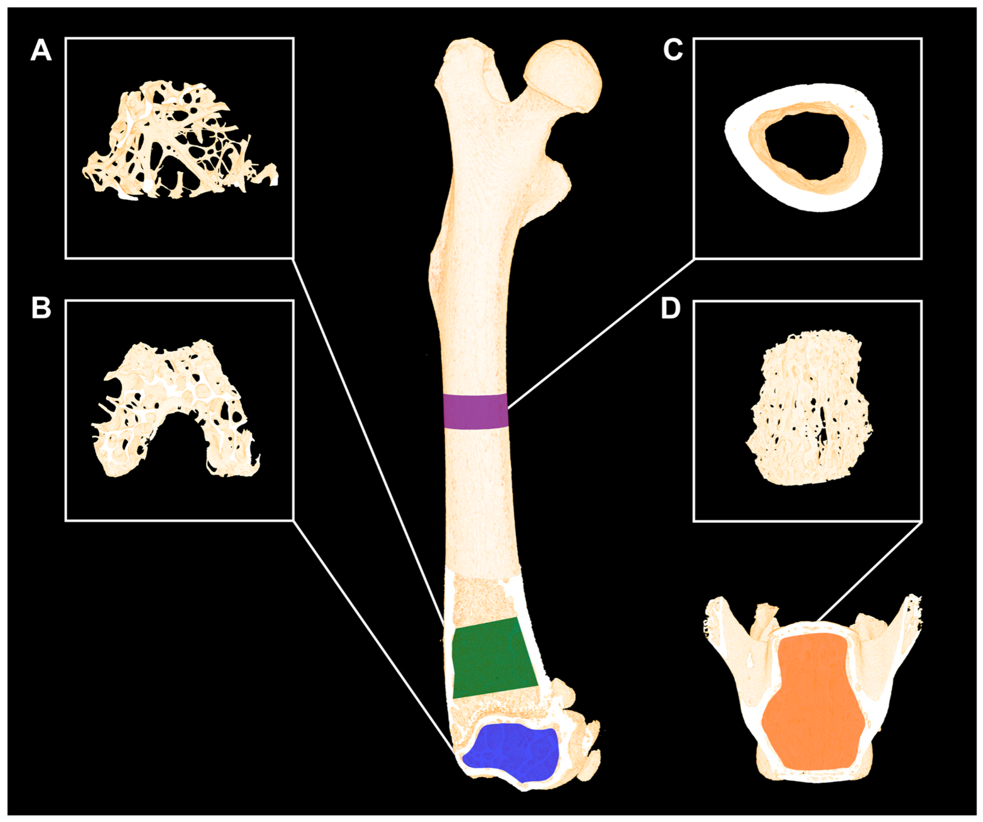
Figure 3.
(A–E) μCT (μCT 35, Scanco Medical, Wangen-Brüttisellen, Switzerland) scans of the same bone using different voxel sizes. The distal femoral metaphysis from a mouse used in a previously published study was scanned using identical settings, except for the voxel size [21]. The scan settings were high-resolution mode (1000 projections/180°), X-ray tube potential of 55 kVp, current of 145 μA, integration time of 800 ms, and isotropic voxel sizes from 3.5 μm to 18.5 μm. Beam hardening effects were reduced using a 0.5 mm aluminum filter. Note how the cortical and trabecular microstructure becomes less well-defined when the voxel size increases and delicate details are lost. Scale bars = 1 mm.
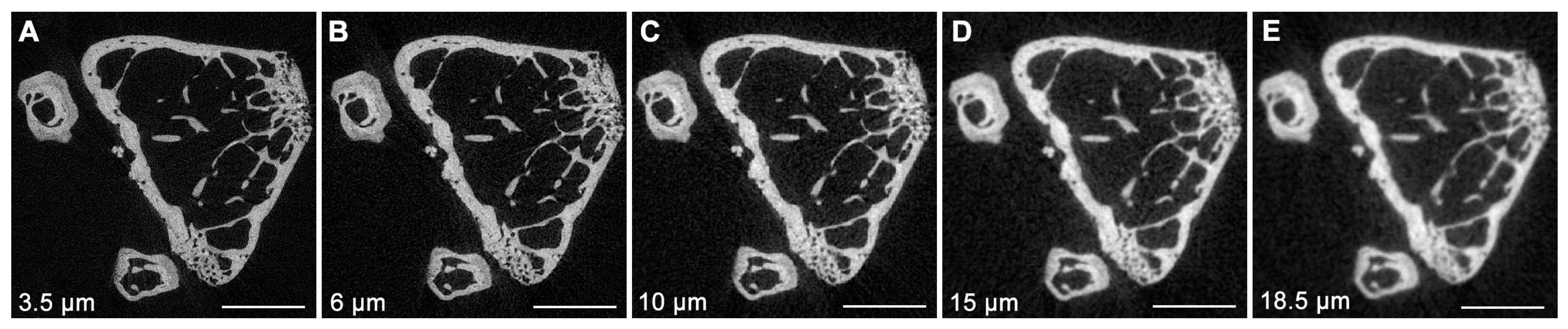
Figure 4.
(A–F) μCT (μCT 35, Scanco Medical, Wangen-Brüttisellen, Switzerland) scans using different integration times. The distal femoral metaphysis from a mouse used in a previously published study was scanned using identical settings, except for the voxel size [21]. The scan settings were high-resolution mode (1000 projections/180°), X-ray tube potential of 55 kVp, current of 145 μA, isotropic voxel size of 3.5 μm, and integration times from 100 ms to 3200 ms (800 ms frame-averaged up to four times). Using a low integration time resulted in an increased signal-to-noise ratio (SNR). The bone segments depicted in the figure were segmented using a fixed threshold of 574 mg HA/cm3. The threshold was identified as the minimum point between the marrow (black) and the bone (white) peak in the attenuation histogram. X-axes on the attenuation histograms are not to scale. Note how higher integration time results in less noise and, therefore, a narrower histogram. Scale bars = 1 mm.
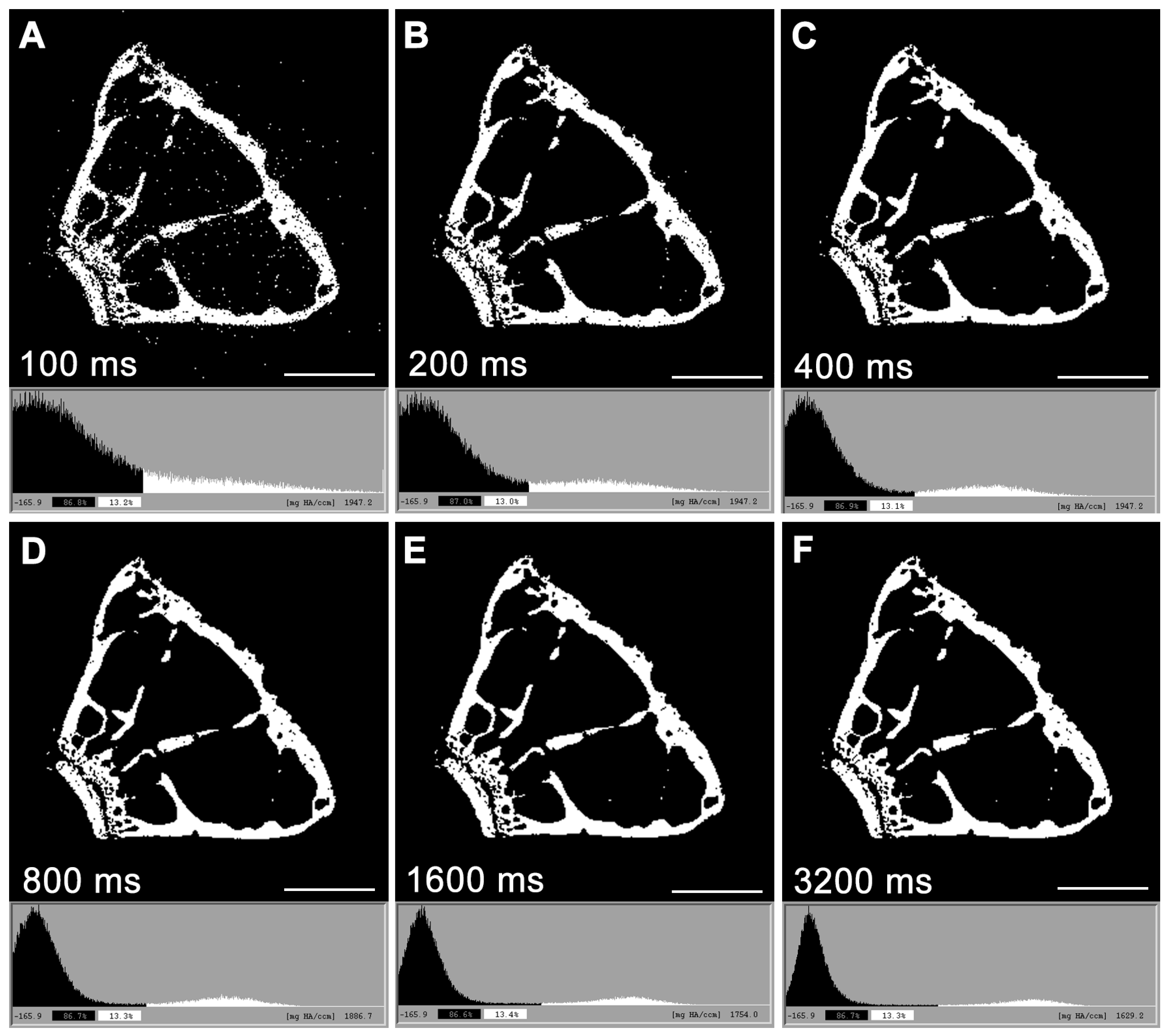
Figure 5.
Three different contouring methods to delineate trabecular bone. (A) Irregular anatomical contouring a few voxels away from the endocortical bone surface. This method is more suitable when morphing the volume of interest (VOI) between slices and minimizes the need for slice-by-slice correction from “line drift” into cortical bone. (B) Irregular anatomical contouring at the very edge of the endocortical bone surface. This method ensures that all trabecular bone is encompassed in the VOI, but it increases the risk of cortical “line drift” when morphing between slices. (C) Regular and uniform, non-anatomical method to contour quickly and easily. A cylindrical VOI is contoured in the middle of the trabecular-rich region of interest. A disadvantage of this method is that a substantial amount of trabecular bone is outside the VOI. Image acquired at 3.5 μm, 55 kVp, 145 mA, and 800 ms integration time (μCT 35, Scanco Medical, Wangen-Brüttisellen, Switzerland). Scale bar = 100 μm.
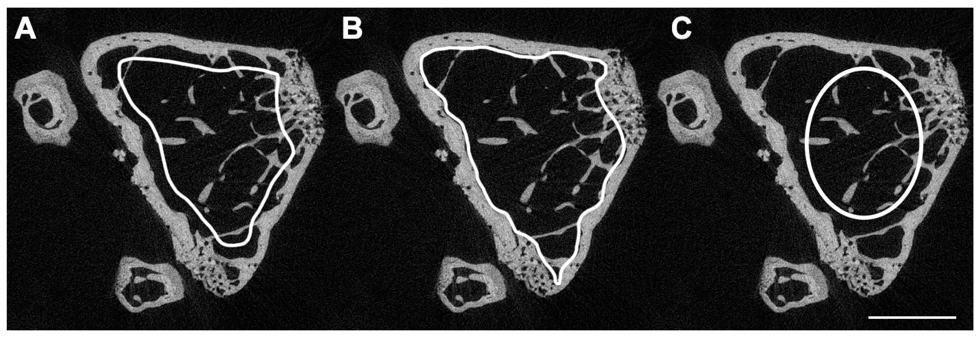
Figure 6.
Dynamic bone histomorphometry at the proximal tibial metaphysis of a rat with botulinum toxin (BTX)-induced hind limb disuse and treated with parathyroid hormone 1–34 (PTH) and growth hormone (GH) in combination [35]. The rat was injected subcutaneously with tetracycline (yellow), calcein (green), and alizarin (red). (A) Note how the pale green autofluorescence (black arrows) can be distinguished from the bright green calcein fluorochrome labels (white arrows). (B) Red HC-mFISH single-band filter. A red single-band filter can be used to enhance the visibility of alizarin fluorochrome labels if they appear dim. Scale bars = 100 μm.
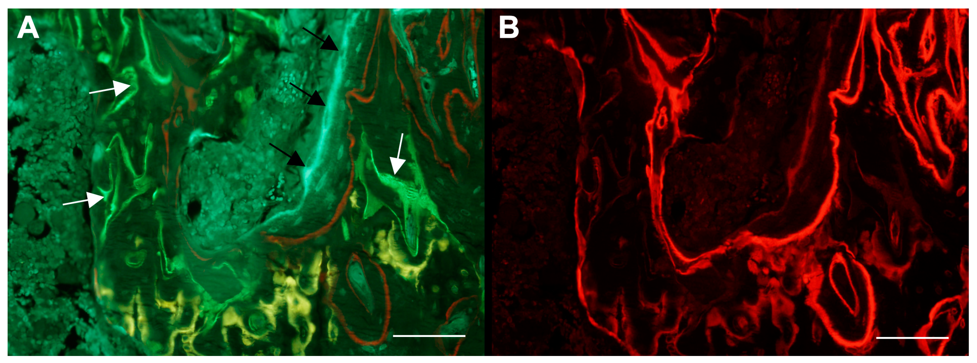
Figure 7.
Simplified illustration of the 3-point bending test of a long bone. (A) The bone is placed on two supporting bars. (B) Vertical load is applied using a rounded bar at the mid-diaphysis. The bottom half of the bone is loaded in tension (red arrows) and the top half is loaded in compression (blue arrows). (C) The fracture starts to develop at the tension side when the maximum load the bone can carry is exceeded. Created with images from Servier Medical Art (https://smart.servier.com (accessed on 1 April 2024)) under a CC BY 3.0 license.
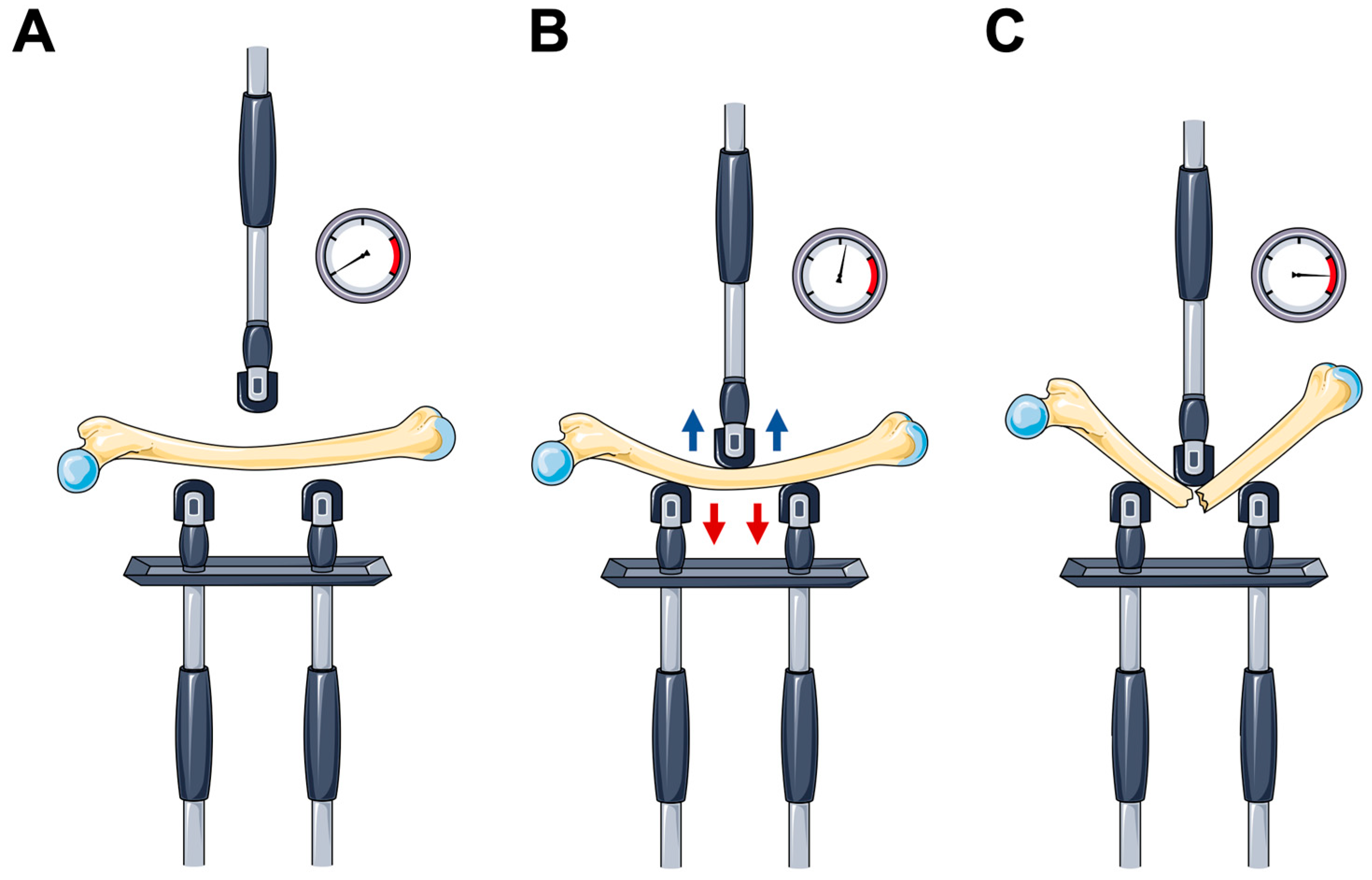
Figure 8.
Load deformation curve from destructive mechanical testing of the femoral neck from a rat [43]. The black circle at the top of the curve (approximately 100 N) marks the maximum load to failure. The yield point is where the curve starts to decrease and separate from the tangent line. The point of tangency (i.e., the point of maximum stiffness) is marked with a black circle (slightly above 40 N) located between two smaller black dots demarking the interval used to compute the tangent line.

Table 1.
Minimum parameters that should be reported for in vivo rodent studies using μCT, μCT scan acquisition, 3D outcomes of trabecular bone microstructure, and cortical morphology. Adapted from Bouxsein et al. [17].
Table 1.
Minimum parameters that should be reported for in vivo rodent studies using μCT, μCT scan acquisition, 3D outcomes of trabecular bone microstructure, and cortical morphology. Adapted from Bouxsein et al. [17].
| Minimum Reporting Requirements for Micro-Computed Tomography (μCT) | ||
|---|---|---|
| μCT scan acquisition | ||
| Variable | Description: | Standard unit |
| Voxel size | Basic discrete 3D unit of μCT image. The 3D volume represents two dimensions within the slice and slice thickness. | μm3 |
| X-ray tube potential (peak) | Applied peak electric potential of X-ray tube that accelerates electrons for generating X-ray photons. | kVp |
| Integration time | Duration of each tomographic projection. | ms |
| Trabecular bone microarchitecture | ||
| Bone volume fraction (BV/TV) | Ratio of the segmented bone volume to the total volume of the region of interest. | % |
| Trabecular number (Tb.N) | Measure of the average number of trabeculae per unit length. | 1/mm |
| Trabecular thickness (Tb.Th) | Mean thickness of trabeculae, assessed using direct 3D methods. | mm |
| Trabecular separation (Tb.Sp) | Mean distance between trabeculae, assessed using direct 3D methods. | mm |
| Cortical morphology | ||
| Total cross-sectional area (Tt.Ar) | Total cross-sectional area inside the periosteal envelope. | mm2 |
| Cortical area (Ct.Ar) | Cortical bone area = cortical volume (Ct.V) ÷ (number of slices × slice thickness). | mm2 |
| Relative cortical bone area to tissue area (Ct.Ar/Tt.Ar) | Cortical area fraction. | % |
| Cortical thickness (Ct.Th) | Average cortical thickness. | mm |
Disclaimer/Publisher’s Note: The statements, opinions and data contained in all publications are solely those of the individual author(s) and contributor(s) and not of MDPI and/or the editor(s). MDPI and/or the editor(s) disclaim responsibility for any injury to people or property resulting from any ideas, methods, instructions or products referred to in the content. |
© 2024 by the author. Licensee MDPI, Basel, Switzerland. This article is an open access article distributed under the terms and conditions of the Creative Commons Attribution (CC BY) license (https://creativecommons.org/licenses/by/4.0/).
Share and Cite
MDPI and ACS Style
Brent, M.B. Imaging, Dynamic Histomorphometry, and Mechanical Testing in Preclinical Bone Research. Osteology 2024, 4, 120-131. https://doi.org/10.3390/osteology4030010
AMA Style
Brent MB. Imaging, Dynamic Histomorphometry, and Mechanical Testing in Preclinical Bone Research. Osteology. 2024; 4(3):120-131. https://doi.org/10.3390/osteology4030010
Chicago/Turabian StyleBrent, Mikkel Bo. 2024. "Imaging, Dynamic Histomorphometry, and Mechanical Testing in Preclinical Bone Research" Osteology 4, no. 3: 120-131. https://doi.org/10.3390/osteology4030010
Article Metrics
Article metric data becomes available approximately 24 hours after publication online.