Hand-Eye Calibration via Linear and Nonlinear Regressions

Abstract

For a robot to pick up an object viewed by a camera, the object’s position in the image coordinate system must be converted to the robot coordinate system. Recently, a neural network-based method was proposed to achieve this task. This methodology can accurately convert the object’s position despite errors and disturbances that arise in a real-world environment, such as the deflection of a robot arm triggered by changes in the robot’s posture. However, this method has some drawbacks, such as the need for significant effort in model selection, hyperparameter tuning, and lack of stability and interpretability in the learning results. To address these issues, a method involving linear and nonlinear regressions is proposed. First, linear regression is employed to convert the object’s position from the image coordinate system to the robot base coordinate system. Next, B-splines-based nonlinear regression is applied to address the errors and disturbances that occur in a real-world environment. Since this approach is more stable and has better calibration performance with interpretability as opposed to the recent method, it is more practical. In the experiment, calibration results were incorporated into a robot, and its performance was evaluated quantitatively. The proposed method achieved a mean position error of 0.5 mm, while the neural network-based method achieved an error of 1.1 mm.

1. Introduction

Vision technologies and robots are employed in various fields, including industry and medicine. In manufacturing, advancements in robot-based automation have addressed the problem of manpower shortage and enabled 24-h production. One common task in robot-based automation is picking up objects viewed by a camera with a robot hand. To accomplish this, precise conversion of object locations from the image coordinate system to the robot coordinate system is required. The general procedure to achieve it involves constructing a precise mathematical model for accurate conversion [1,2,3,4,5,6] and optimizing this model through calibration [7,8,9,10,11,12,13,14,15], known as hand-eye calibration. This can be accomplished by taking images of a board with a specific pattern, such as a checkerboard pattern, from various positions and then using the image group taken to optimize a mathematical model.

However, a reported drawback to precise mathematical models is that they lack robust responses to the various changes and errors found in real environments [16,17]. For example, if calibration is based upon structure from motion, then incorrect feature correspondences often arise in real environments, causing large camera posture estimation errors [18]. In addition, robot structural deflections complicating accurate co-registration of robot arms and vision systems have been reported [19]. Thus, expressing all the errors that might occur in a real environment by a mathematical model could significantly reduce robot hand location errors. However, this is difficult. Recently, an approach has been proposed to address these problems using a neural network [16]. This approach involves training a neural network to convert an object’s location in the image coordinate system into the robot coordinate system accurately. Using the learning data, including various errors acquired in real environments, and a neural network with high expressivity makes robust conversion possible. This process has the advantage of simplicity since it no longer requires the design of complicated mathematical models while enabling end-to-end learning, thus simplifying its use. However, as learning results depend on the type of network model and hyperparameters, learning results are unstable and low in explainability.

To solve these problems, this study proposes a regression-based approach using data acquired in real-world environments. A linear regression model is used to convert object positions from the image coordinate system to the robot coordinate system, and a nonlinear regression model based on B-splines is used to handle errors that cannot be handled by linear regression. Using both linear and nonlinear regressions simplifies the calculation and results in more accurate conversion with better stability. In the experiments, the proposed method was compared to three neural network models with different structures in terms of calibration performance. The calibration results were used to operate a robot and evaluated. The proposed method has the following advantages:

• The proposed method has more stability and explainability than the neural network-based method because the regression equations are obtained;
• The proposed approach needs reduced effort because the number of hyperparameters, which must be adjusted by a user, is smaller;
• Compared to the approach based on the neural network, the proposed method can achieve better calibration performance.

2. Related Work

Several studies conducted on hand-eye calibration have adopted the approach of designing a mathematical model [1,2,3,4,5,6]. A basic model example is $AX=XB$ [4]. A and B are both homogeneous transformation matrices, respectively, expressing the relative motions of a camera attached to a robot hand. X is a transformation matrix between a camera and hand that must be estimated through calibration. The general procedure includes capturing images of a board with a specific pattern, such as a checkerboard, and optimizing the model using the captured image set. Several mathematical models and calibration boards [20] have been proposed to achieve more accurate and faster calibration. To optimize the mathematical model, there are two main approaches, which are the separation and simultaneous methods. In the former, a rotation matrix of X and translation vector are optimized separately [7,8,9,10,11]. In the latter, both are solved for simultaneously [12,13,14,15].

Recent research related to hand-eye calibration is reviewed next. Fu et al. developed constrained least squares and nonlinear calibration models that consider the effect of robot pose error [21]. Calibration for high-precision robotic machining was achieved by selecting rotation parameters that have a significant impact on solution accuracy. Do et al. addressed the recognition of six degrees of freedom for workpieces using an RGB-D camera to automate robot picking and placing for production works [22]. For accurate grasping, robot error compensation using a checkerboard was introduced. In this compensation, a polynomial fitting algorithm was used to reduce errors. Su et al. developed a calibration method to manipulate products with variable height using a robot [23]. They experimentally calibrated a rigid transformation model and considered distortion in the camera lens. The four-point calibration method with a calibration plate set at different heights was applied to calculate the rigid transformation matrix. Dekel et al. proposed a least squares formulation using dual quaternions and efficient optimization algorithms to solve a noisy hand-eye calibration problem [24]. In this approach, a global minimum is guaranteed by using only a 1D line search of a convex function. Yang et al. developed a tool center point (TCP) calibration method without the need for external tools [25]. The efficiency and accuracy of TCP calibration were achieved by establishing a constraint model and minimizing reprojection error. Zhang et al. proposed a calibration method using a time-of-flight camera [26]. After capturing a calibration board from different robot poses, the calibration using singular value decomposition was performed to achieve stable manipulation. Kalia et al. developed a method for accurate medical augmented reality [27]. In this method, a procedure of hand-eye calibration was divided into pre-operative and intra-operative steps. Accurate calibration is possible by utilizing information that a camera position does not change drastically. Valassakis et al. solved a calibration problem using learning-based methods from a single RGB image [28]. The developed models predict an extrinsic matrix from an image and regress 2D keypoints, depth, and segmentation maps, achieving better performance than other approaches. Lembono et al. proposed a calibration method that simultaneously improves kinematic parameters of six degrees of freedom and extrinsic parameters of a 2D laser range finder [29]. A flat plate was located around the robot, and calibration parameters were optimized using geometric planar constraints, which reduced average position and orientation errors.

In addition to the above studies, some methods not based on mathematical models have been proposed [2,16]. One of the reasons for adopting these approaches is the complexity of mathematical models accounting for the various noise and errors in real environments. Examples include mismatching of feature points in structure from motion [18] and robot arm deflection [19]. Using data including noise and errors acquired in real environments and learning a network model with high expressivity enables robust conversion; this approach is expressed by $B=f_{\mathrm{NN}}\left(A\right)$. A is the location of an object in the image coordinate system, $f_{\mathrm{NN}}$ is a neural network, and B is the result of A converted with a neural network and expresses the location in the robot coordinate system. This approach enables preparing learning data while a network model enables calibration, thus simplifying its use.

However, this approach has several disadvantages. For example, it is difficult to find which model structure is best. In addition, hyperparameter adjustment is time- and labor-intensive, and there is no stability to final calibration results. Moreover, the network model is low in explainability. Therefore, this study proposes a linear and nonlinear regression-based approach. First, a linear regression model is trained using data acquired in a real environment to convert the location from the image coordinate system to the robot coordinate system. Then, a nonlinear regression model is trained to further minimize the conversion error. By combining these models in a coarse-to-fine manner, the stability and accuracy of the calibration process are improved, and the results are highly explainable. The hyperparameter selection problem is also avoided. This new approach can be expressed as $B=f_{\mathrm{NLR}}\left(f_{\mathrm{LR}}\left(A\right)\right)$; $f_{\mathrm{LR}}$ is a linear regression model and $f_{\mathrm{NLR}}$ is a nonlinear regression model. The details of this procedure are described below.

3. Proposed Method

Algorithm 1 summarizes the logical flow of the proposed method. First, data to be used for regression analysis are created using a robot and tablet terminal. Next, linear regression is employed to convert a position in the image coordinate system to the robot base coordinate system using the data. To reduce error in the linear regression, nonlinear regression based on B-splines is applied. To minimize the error as much as possible, the control points are optimized using an evolutionary computation technique, artificial bee colony (ABC). Finally, the obtained calibration results are used for evaluation using the robot.

Algorithm 1 Flow of the proposed method.

1: // Regression phase 2: Data creation using a robot and tablet terminal for regression analysis (Section 3.1) 3: Linear regression to transform the coordinate system (Section 3.2) 4: while Not end of iteration do 5:    Nonlinear regression based on B-splines (Section 3.3) 6:    Optimization of control points to minimize error by ABC (Section 3.3.1) 7: // Evaluation phase 8: Evaluation of the calibration results using a robot (Section 4)

3.1. Preparation

In the neural network-based method proposed by Hua et al. [16], the preliminary preparation involves taking images of a checkerboard with a camera and acquiring multiple corner coordinates in the image coordinate system (${\Sigma }_I$). This coordinate group corresponds to A in $B=f_{\mathrm{NN}}\left(A\right)$. Subsequently, a robot is manually operated such that a manipulator tip touches one corner, and the hand location in a robot coordinate system is acquired (${\Sigma }_R$). B is obtained when this data acquisition is performed for all corners. By using A as the learning data and B as the ground truth to learn a neural network ($f_{\mathrm{NN}}$), it is possible to directly convert location in the image coordinate system into the robot coordinate system.

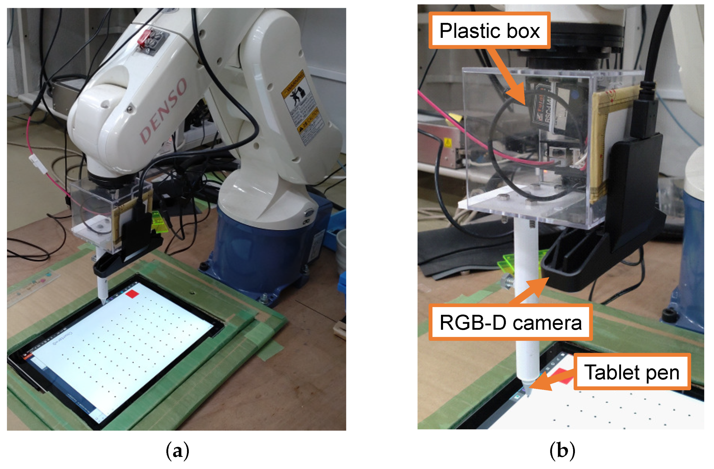
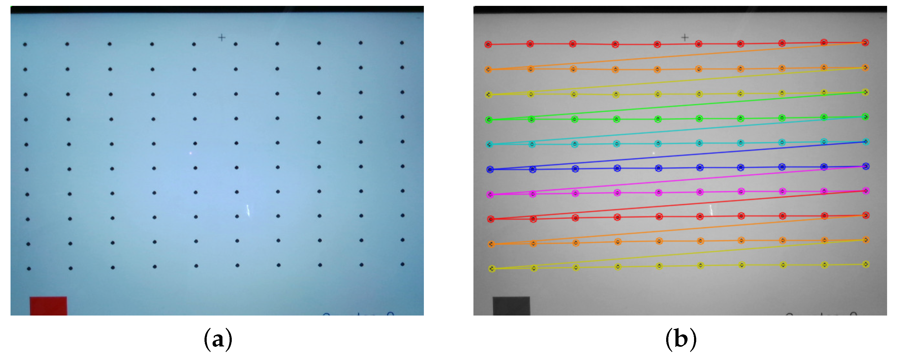
The proposed method necessitates the prior preparation of A and B as shown in Figure 1. Considering this requirement, a system was constructed, as shown in Figure 2a. A 6-axis articulated robot (DENSO VP-6242 [30]) and a tablet terminal (Surface Pro 7 (Microsoft, Redmond, WA, USA)), instead of a checkerboard, were used. This reason is explained later. Figure 2b shows the details of the end-effector. A plastic box was attached to the hand tip, with an RGB-D camera and tablet pen further attached to this box. To acquire A, 100 black dots were displayed in Figure 3a. Tablet images were taken using an RGB-D camera. In this study, calibration was performed for tasks, such as bolt picking in Furukawa et al. [31], and the workspace accounts for the area were covered with black dots. The attached camera was an Intel RealSense SR300; thus, there was no need to account for image distortion [32]. When images were taken, OpenCV [33] was used to acquire the location at the black dot ${\Sigma }_I$ (Figure 3b). To acquire B, the robot hand was manually manipulated such that one black dot and the tablet pen tip touched. Thus, the hand location in ${\Sigma }_R$ was acquired. By performing this for all black dots, it is possible to acquire B.

When the prepared A and B are plotted, they appear as in Figure 4. Both distributions are the same, but there are several points to note. First, the units are different. Therefore, while A is the image coordinate system and has a unit of px, B is the robot coordinate system with a unit of millimeters. To account for this difference in units, the location in ${\Sigma }_I$, which is conventionally based on a pinhole camera model, is converted into the camera coordinate system in millimeters. Then, a mathematical model is used to convert it into a location in ${\Sigma }_R$ [2,16]. In contrast, the method proposed by Hua et al. and the proposed method perform direct conversion with a neural network ($f_{\mathrm{NN}}$) or linear and nonlinear regression ($f_{\mathrm{LR}}$ and $f_{\mathrm{NLR}}$) without the need for the above procedure. Second, errors occur when preparing B, making it difficult to manipulate the robot hand manually such that the black dots and pen tip exactly match, resulting in frequent small errors. Although preparing an error-free B is time-consuming, it is not realistic due to the intensive labor involved. Consequently, calibration using data that include such errors is required.

3.2. Linear Regression

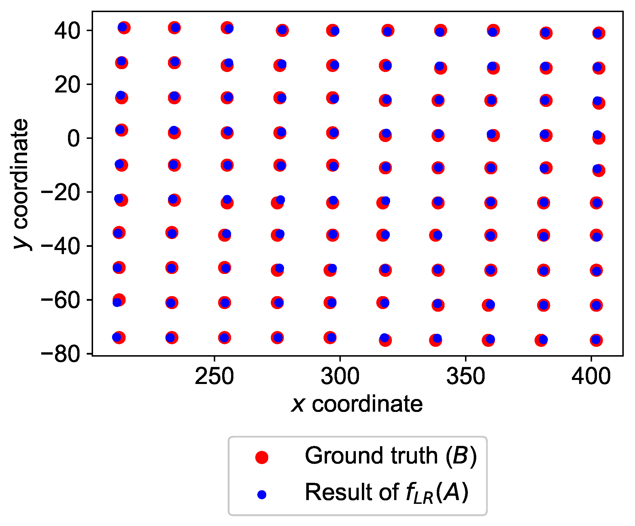
As shown in Figure 4, the distributions of A and B are the same. Therefore, linear regression analysis can be used to obtain $f_{\mathrm{LR}}$ by converting the location in ${\Sigma }_I$ (${(x_i^{\prime },y_i^{\prime })}^T$) into ${\Sigma }_R$. Figure 5 shows an example of conversion results; while the conversion is generally accurate, many mislocating errors are present due to errors in the ground truth B. As the misplacement direction was irregular, it was difficult to transform the results of $f_{\mathrm{LR}}\left(A\right)$ such that errors at all points were minimized by affine transformation or perspective projection transformation. To overcome this problem, nonlinear regression analysis ($f_{\mathrm{NLR}}$) based on B-splines was applied in this method.

3.3. Nonlinear Regression Based on B-Splines

The deformation based on B-splines can realize the deformation that cannot be realized by affine transformation and perspective projection transformation [34,35]. The specific formula is shown below.

$$\begin{array}{ccc}\hfill {\mathbf{p}}_i^{\prime }& =& f_{\mathrm{NLR}}\left({\mathbf{p}}_i\right)=\sum _{n=0}^3\sum _{m=0}^3{f}_m\left(u\right)f_n\left(v\right){\mathbf{c}}_{j+m,k+n}\hfill \end{array}$$

(1)

$$\begin{array}{ccc}\hfill u& =& \left(x_i-x_{j+m,k+n}^c\right)/w\hfill \end{array}$$

(2)

$$\begin{array}{ccc}\hfill v& =& \left(y_i-y_{j+m,k+n}^c\right)/h\hfill \end{array}$$

(3)

$$\begin{array}{ccc}\hfill f_0\left(t\right)& =& {\left(1-t\right)}^3/6\hfill \end{array}$$

(4)

$$\begin{array}{ccc}\hfill f_1\left(t\right)& =& \left(3t^3-6t^2+4\right)/6\hfill \end{array}$$

(5)

$$\begin{array}{ccc}\hfill f_2\left(t\right)& =& \left(-3t^3+3t^2+3t+1\right)/6\hfill \end{array}$$

(6)

$$\begin{array}{ccc}\hfill f_3\left(t\right)& =& t^3/6\hfill \end{array}$$

(7)

The above equations are explained in Figure 6. ${\mathbf{p}}_i={(x_i,y_i)}^T$ represents the coordinates of the ith black dot converted by $f_{\mathrm{LR}}$. Moving these using the control points (${\mathbf{c}}_{j+m,k+n}={(x_{j+m,k+n}^c,y_{j+m,k+n}^c)}^T$) represented by gray squares is considered. First, $4\times 4$ enclosing control points with ${\mathbf{p}}_i$ at the center are selected. If the number of control points arranged in the horizontal and vertical directions is J and K, respectively, the top-left control point is expressed by ${\mathbf{c}}_{j,k}$ ($j\in [0,J-1]$, $k\in [0,K-1]$). Consequently, each of the $4\times 4$ control points are expressed by ${\mathbf{c}}_{j+m,k+n}$ ($m,n\in [0,3]$). Subsequently, Equations (2) and (3) are used to determine u and v. w and h are the width and height between adjacent control points, respectively. Inputting u and v into cubic B-splines basis functions ($f_m$,$f_n$), it is possible to obtain the converted coordinate (${\mathbf{p}}_i^{\prime }$). In the proposed method, the artificial bee colony (ABC)—an evolutionary computation method—is used to optimize the location of all control points such that these coordinates are as close as possible to B, which is the ground truth.

3.3.1. Optimization of Control Point Locations with ABC

ABC [36], proposed by Sato et al., is used in the proposed method to optimize the locations of the control point group. ABC is an evolutionary computation method with a higher search performance than other population-based metaheuristic algorithms in deformation parameter estimation tasks for image alignment [37]. It also has the advantage of adjusting fewer hyperparameters by trial and error in advance. For these reasons, the ABC proposed by Sato et al. is adopted.

Algorithm 2 shows the procedure for using this ABC to optimize control point locations. First, a target point group resulting from $f_{\mathrm{LR}}\left(A\right)$ and ground truth B is used as input. Next, $J\times K$ control points are arranged. Then, the search range of the control points, number of individuals, and generations that are the hyperparameters of ABC are set. The arrangement of the control point group in ABC is arranged such that it minimizes the fitness function (F). The fitness function used is the sum of the Euclidean distances between the point group moved by the optimized control points and each point (${\mathbf{p}}_i^{\mathrm{GT}}$) of B, which is the ground truth, as shown below.

$$\begin{array}{c}\hfill F=\sum _{i=0}^{99}{\left|\left|{\mathbf{p}}_i^{\prime }-{\mathbf{p}}_i^{\mathrm{GT}}\right|\right|}_2\end{array}$$

(8)

Algorithm 2 Optimization by artificial bee colony (ABC).

1: Input target points (result of $f_{\mathrm{LR}}\left(A\right)$) and ground truth (B) 2: Place $J\times K$ control points 3: Set search range of the control points and hyperparameters of ABC 4: Optimize the control point locations based on a fitness function

Figure 7 shows an example of optimization results. By comparing (a) with (b), the arrangement of the control points indicated by the green squares has changed. In (b), the points where the error is less than the result of $f_{\mathrm{LR}}\left(A\right)$ due to the introduction of nonlinear regression are rendered in cyan. In this example, the $3/4$ error is reduced, indicating that the introduction of nonlinear regression contributes to further error reduction.

4. Experiment

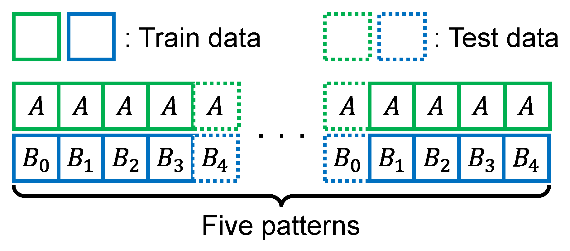
One A and five B were prepared to evaluate the proposed method and a comparative method through the five-fold cross validation (Figure 8). Four learning datasets for learning regression analysis or a neural network model were used. Then, each of the learning results was evaluated using one remaining dataset as test data. Equation (8) was used to evaluate the learning results by test data.

In linear regression analysis in the proposed method, Equation (9) was employed.

$$\begin{array}{c}\hfill \left[\begin{array}{c}{x}_i\\ y_i\end{array}\right]=\left[\begin{array}{cc}{\alpha }_{00}& {\alpha }_{01}\\ {\alpha }_{10}& {\alpha }_{11}\end{array}\right]\left[\begin{array}{c}{x}_i^{\prime }\\ y_i^{\prime }\end{array}\right]+\left[\begin{array}{c}{\beta }_0\\ {\beta }_1\end{array}\right]\end{array}$$

(9)

Here, $\alpha$ and $\beta$ are the coefficients and intercepts estimated by regression analysis, respectively. The three models shown in Figure 9 were prepared as the comparative neural network model. In order to compare the proposed method with that of Hua and Zeng [16], it would have been ideal to reproduce their model. However, detailed information was not provided in their paper, making replication difficult. I considered alternative models, but the number of hyperparameters is too large and this is not the main objective of this study. Considering this reason and the fact that the dataset used in this study does not have a complex distribution, as shown in Figure 4, the simple three models shown in Figure 9 were prepared and compared. They are capable of linear and nonlinear regressions like the proposed method. The number of weights affects regression performance. However, it is difficult to predict in advance the best number of weights for hand-eye calibration. Therefore, models with three different numbers of weights were prepared. These models were developed previously by the author through trial and error and have good performance. A mean squared error loss function was set for learning. For the optimizer, Adam [38] was used, and a learning coefficient of 0.01 was set. The number of epochs was 5000.

The individual size of ABC used in control point optimization was set to a sufficiently large value of 1000 to avoid falling into a local solution. The number of evaluations for the fitness function was set to $3\times {10}^6$. The number of control points arranged in the horizontal and vertical directions (J and K) was 14 and 13, respectively. Therefore, the number of dimensions of variables optimized by ABC was $14\times 13\times 2=364$. The horizontal and vertical distances (w and h) between adjacent control points were 20 and 14, respectively. The search range of each optimized control point was $[-5,5]$.

4.1. Results and Discussion

4.1.1. Five-Fold Cross Validation (CV)

Table 1. Results of five-fold cross validation (CV).

	Mean Distance Error (mm)
CV	${\mathit{f}}_{\mathbf{NLR}}\left({\mathit{f}}_{\mathbf{LR}}\right)$	${\mathit{f}}_{\mathbf{LR}}$	${\mathit{f}}_{\mathbf{NN}}$ (Model 1)	${\mathit{f}}_{\mathbf{NN}}$ (Model 2)	${\mathit{f}}_{\mathbf{NN}}$ (Model 3)
1	0.53	0.69	1.08	0.80	0.86
2	0.57	0.70	0.71	0.79	4.64
3	0.61	0.66	1.44	0.88	5.08
4	0.66	0.67	1.65	1.61	2.84
5	0.64	0.68	2.15	1.98	5.67
Ave.	0.60	0.68	1.40	1.21	3.82
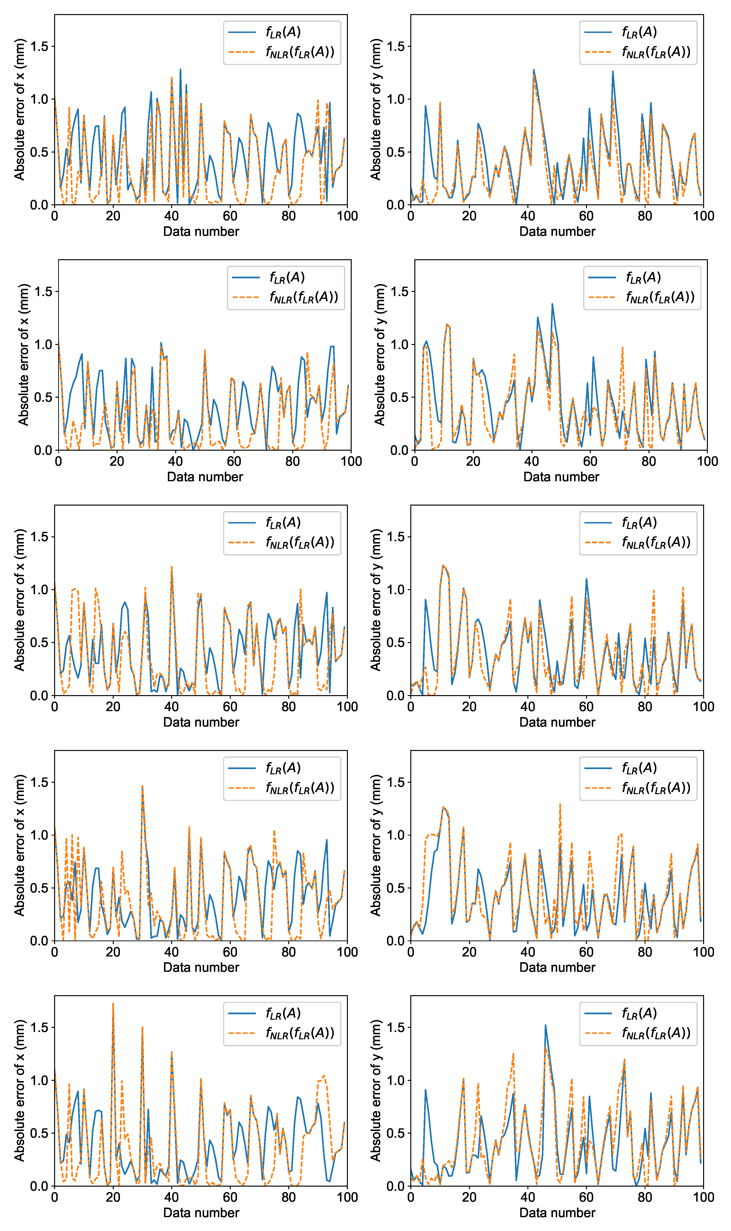
SD	0.04	0.01	0.49	0.49	1.76

shows the results of five-fold CV. When comparing $f_{\mathrm{LR}}$, which performs only linear regression, and a neural network-based method ($f_{\mathrm{NN}}$), the former has a smaller mean test data error. In addition, minimal error variance was observed. Consequently, the linear regression model has higher stability. In addition, the neural network model was equal to that of the linear regression model in results. However, the large variance in results resulted in poor stability.

Table 2. Acquired partial regression coefficients and constants by the linear regression analysis.

CV	Partial Regression Coefficients	Constants
1	$\left[\begin{array}{cc}3.3\times {10}^{-1}& 8.1\times {10}^{-4}\\ -6.8\times {10}^{-5}& 3.3\times {10}^{-1}\end{array}\right]$	$\left[\begin{array}{c}203.8\\ -93.4\end{array}\right]$
2	$\left[\begin{array}{cc}3.3\times {10}^{-1}& 8.4\times {10}^{-4}\\ -5.6\times {10}^{-6}& 3.3\times {10}^{-1}\end{array}\right]$	$\left[\begin{array}{c}203.8\\ -93.4\end{array}\right]$
3	$\left[\begin{array}{cc}3.3\times {10}^{-1}& 9.8\times {10}^{-4}\\ 1.1\times {10}^{-6}& 3.3\times {10}^{-1}\end{array}\right]$	$\left[\begin{array}{c}203.7\\ -93.4\end{array}\right]$
4	$\left[\begin{array}{cc}3.3\times {10}^{-1}& 9.6\times {10}^{-4}\\ -9.6\times {10}^{-5}& 3.3\times {10}^{-1}\end{array}\right]$	$\left[\begin{array}{c}203.7\\ -93.5\end{array}\right]$
5	$\left[\begin{array}{cc}3.3\times {10}^{-1}& 9.0\times {10}^{-4}\\ -1.4\times {10}^{-4}& 3.3\times {10}^{-1}\end{array}\right]$	$\left[\begin{array}{c}203.7\\ -93.4\end{array}\right]$

lists the partial regression coefficient and constant term obtained by linear regression analysis using the learning data. By comparing the result of applying the nonlinear regression formula based on B-splines to the obtained linear regression formula ($f_{\mathrm{NLR}}\left(f_{\mathrm{LR}}\right)$), the mean distance error was smaller than $f_{\mathrm{LR}}$. Consequently, nonlinear regression contributes to the further reduction in error. Figure 10 shows the absolute errors of x and y directions by $f_{\mathrm{LR}}\left(A\right)$ and $f_{\mathrm{NLR}}\left(f_{\mathrm{LR}}\left(A\right)\right)$, respectively. Not all, but many errors were decreased.

4.1.2. Evaluation Using Robot

Subsequently, the calibration results obtained through each method were evaluated by introducing them to the robot hand shown in Figure 2. A hand holding a tablet pen touched 100 black dots displayed on the tablet screen, and the mean touch error was obtained. As a tablet terminal was used, it is possible to measure the distance error of the ground truth black dots and touched locations. The obtained results were in px units and can be converted to mm using the following formula:

$$\begin{array}{c}\hfill p_{\mathrm{mm}}=p_{\mathrm{px}}\times \frac{25.4}{\mathrm{PPI}}\times s,\end{array}$$

(10)

where $p_{\mathrm{mm}}$, $p_{\mathrm{px}}$, PPI, and s are the converted result in mm, position in pixel, pixel per inch, and display scale of the tablet computer, respectively. The PPI and s depend on a used tablet computer. In the developed system, $\mathrm{PPI}=267$ and $s=2$ were set. For $f_{\mathrm{NN}}$, the experimentation was conducted using Model 2, which had the smallest error, with the results listed in Table 1.

Even in the experiment using a robot (

Table 3. Evaluation results for each calibration method using robot.

	Mean Touching Error
Method	px	mm
$f_{\mathrm{NLR}}\left(f_{\mathrm{LR}}\right)$	2.63	0.50
$f_{\mathrm{LR}}$	4.12	0.78
$f_{\mathrm{NN}}$ (Model 2)	5.79	1.10

), the mean touch error of $f_{\mathrm{NLR}}\left(f_{\mathrm{LR}}\right)$ was the smallest. Compared to $f_{\mathrm{LR}}$, the error was reduced by 0.28 mm. Consequently, introducing nonlinear regression contributes to error reduction. In addition, the neural network model mean touch error was 1 mm or more. If other network structures or models were used, this error may be even smaller. However, several structures and models have been previously proposed and selecting the optimal model for the tasks in this study was not easy. Even tentative selection requires the adjustment of various parameters at then time of learning. When these points are considered, fewer hyperparameters in the proposed method must be considered, thus making it stable and robustly responsive to differences in learning data. The mean touching error of $f_{\mathrm{NLR}}\left(f_{\mathrm{LR}}\right)$ was not a great achievement compared to the position repeatability of the used robot ($\pm 0.02$ mm [30]). However, the error was the smallest compared to the other methods. Consequently, when comprehensively assessed, the approach in the proposed method has higher performance than a neural network-based approach.

5. Conclusions

This study attempted to construct a method with improved stability and better performance than the recently proposed neural network-based hand-eye calibration. A neural network uses high expressivity and can directly convert locations in the image coordinate system to the robot coordinate system. However, the learning results are not stable. Therefore, the proposed method focuses on regression analysis to address the stability problem. As the linear regression of data, including various noise and error, is insufficient, nonlinear regression based on B-splines has been introduced. When learning results were introduced to a robot and the touch error was measured, the regression-based hand-eye calibration could achieve higher stability and lower touch error than that of the neural network-based model. In addition, linear regression analysis error could be further reduced by introducing nonlinear regression analysis.

In future work, the method must be improved to further reduce error. In addition, a method that takes into account 3D space will be constructed. The reason for this is that it is necessary when considering assembly automation in 3D space using robots.

References

1. Sato, J. Hand-Eye Calibration Using a Tablet Computer. Math. Comput. Appl. 2023, 28, 22. [Google Scholar] [CrossRef]
2. Enebuse, I.; Foo, M.; Ibrahim, B.S.K.K.; Ahmed, H.; Supmak, F.; Eyobu, O.S. A Comparative Review of Hand-Eye Calibration Techniques for Vision Guided Robots. IEEE Access 2021, 9, 113143–113155. [Google Scholar] [CrossRef]
3. Jiang, J.; Luo, X.; Luo, Q.; Qiao, L.; Li, M. An Overview of Hand-Eye Calibration. Int. J. Adv. Manuf. Technol. 2022, 22, 77–97. [Google Scholar] [CrossRef]
4. Shiu, Y.C.; Ahmad, S. Calibration of wrist-mounted robotic sensors by solving homogeneous transform equations of the form AX = XB. IEEE Trans. Robot. Autom. 1989, 5, 16–29. [Google Scholar] [CrossRef]
5. Motai, Y.; Kosaka, A. Hand-Eye Calibration Applied to Viewpoint Selection for Robotic Vision. IEEE Trans. Ind. Electron. 2008, 55, 3731–3741. [Google Scholar] [CrossRef]
6. Zhuang, H.; Roth, Z.; Sudhakar, R. Simultaneous robot/world and tool/flange calibration by solving homogeneous transformation equations of the form AX = YB. IEEE Trans. Robot. Autom. 1994, 10, 549–554. [Google Scholar] [CrossRef]
7. Tsai, R.Y.; Lenz, R.K. A new technique for fully autonomous and efficient 3D robotics hand/eye calibration. IEEE Trans. Robot. Autom. 1989, 5, 345–358. [Google Scholar] [CrossRef]
8. Wang, C.C. Extrinsic calibration of a vision sensor mounted on a robot. IEEE Trans. Robot. Autom. 1992, 8, 161–175. [Google Scholar] [CrossRef]
9. Park, F.C.; Martin, B.J. Robot sensor calibration: Solving AX = XB on the Euclidean group. IEEE Trans. Robot. Autom. 1994, 10, 717–721. [Google Scholar] [CrossRef]
10. Ma, S.D. A self-calibration technique for active vision systems. IEEE Trans. Robot. Autom. 1996, 12, 114–120. [Google Scholar]
11. Daniilidis, K. Hand-Eye Calibration Using Dual Quaternions. Int. J. Robot. Res. 1999, 18, 286–298. [Google Scholar] [CrossRef]
12. Horaud, R.; Dornaika, F. Hand-Eye Calibration. Int. J. Robot. Res. 1995, 14, 195–210. [Google Scholar] [CrossRef]
13. Andreff, N.; Horaud, R.; Espiau, B. Robot Hand-Eye Calibration using Structure from Motion. Int. J. Robot. Res. 2001, 20, 228–248. [Google Scholar] [CrossRef]
14. Zhao, Z. Hand-eye calibration using convex optimization. In Proceedings of the International Conference on Robotics and Automation, Shanghai, China, 9–13 May 2011; pp. 2947–2952. [Google Scholar]
15. Heller, J.; Havlena, M.; Pajdla, T. Globally Optimal Hand-Eye Calibration Using Branch-and-Bound. IEEE Trans. Pattern Anal. Mach. Intell. 2016, 38, 1027–1033. [Google Scholar] [CrossRef] [PubMed]
16. Hua, J.; Zeng, L. Hand-Eye Calibration Algorithm Based on an Optimized Neural Network. Actuators 2021, 10, 85. [Google Scholar] [CrossRef]
17. Sun, W.; Liu, J.; Zhao, Y.; Zheng, G. A Novel Point Set Registration-Based Hand-Eye Calibration Method for Robot-Assisted Surgery. Sensors 2022, 22, 8446. [Google Scholar] [CrossRef]
18. Zhi, X.; Schwertfeger, S. Simultaneous Hand-Eye Calibration and Reconstruction. In Proceedings of the IEEE/RSJ International Conference on Intelligent Robots and Systems, Vancouver, BC, Canada, 24–28 September 2017; pp. 1470–1477. [Google Scholar]
19. Wang, Z.; Liu, Z.; Ma, Q.; Cheng, A.; Hui Liu, Y.; Kim, S.; Deguet, A.; Reiter, A.; Kazanzides, P.; Taylor, R.H. Vision-Based Calibration of Dual RCM-Based Robot Arms in Human-Robot Collaborative Minimally Invasive Surgery. IEEE Robot. Autom. Lett. 2018, 3, 672–679. [Google Scholar] [CrossRef]
20. Lin, W.; Liang, P.; Luo, G.; Zhao, Z.; Zhang, C. Research of Online Hand-Eye Calibration Method Based on ChArUco Board. Sensors 2022, 119, 3805. [Google Scholar] [CrossRef]
21. Fu, J.; Ding, Y.; Huang, T.; Liu, X. Hand-eye calibration method with a three-dimensional-vision sensor considering the rotation parameters of the robot pose. Int. J. Adv. Robot. Syst. 2020, 17, 1–13. [Google Scholar] [CrossRef]
22. Do, Q.T.; Chang, W.Y.; Chen, L.W. Dynamic Workpiece Modeling with Robotic Pick-Place Based on Stereo Vision Scanning Using Fast Point-Feature Histogram Algorithm. Appl. Sci. 2021, 11, 11522. [Google Scholar] [CrossRef]
23. Su, S.; Gao, S.; Zhang, D.; Wang, W. Research on the Hand-Eye Calibration Method of Variable Height and Analysis of Experimental Results Based on Rigid Transformation. Appl. Sci. 2022, 12, 4415. [Google Scholar] [CrossRef]
24. Dekel, A.; Häenstam-Nielsen, L.; Caccamo, S. Optimal least-squares solution to the hand-eye calibration problem. In Proceedings of the IEEE/CVF Conference on Computer Vision and Pattern Recognition (CVPR’2020), Seattle, WA, USA, 13–19 June 2020; pp. 13595–13603. [Google Scholar]
25. Yang, Z.; Gong, L.; Liu, C. Efficient TCP Calibration Method for Vision Guided Robots Based on Inherent Constraints of Target Object. IEEE Access 2021, 9, 8902–8911. [Google Scholar] [CrossRef]
26. Zhang, X.; Yao, M.; Cheng, Q.; Liang, G.; Fan, F. A novel hand-eye calibration method of picking robot based on TOF camera. Front. Plant Sci. 2023, 13, 1099033. [Google Scholar] [CrossRef] [PubMed]
27. Kalia, M.; Mathur, P.; Navab, N.; Salcudean, S.E. Marker-less real-time intra-operative camera and hand-eye calibration procedure for surgical augmented reality. Healthc. Technol. Lett. 2019, 6, 255–260. [Google Scholar] [CrossRef] [PubMed]
28. Valassakis, E.; Drezckowski, K.; Johns, E. Learning Eye-in-Hand Camera Calibration from a Single Image. In Proceedings of the Conference on Robot Learning (CoRL’2021), Virtual, 8–11 November 2021; pp. 1–11. [Google Scholar]
29. Lembono, T.S.; Suárez-Ruiz, F.; Pham, Q.C. SCALAR: Simultaneous Calibration of 2D Laser and Robot Kinematic Parameters Using Planarity and Distance Constraints. In Proceedings of the IEEE/RSJ International Conference on Intelligent Robots and Systems (IROS’2018), Madrid, Spain, 1–5 October 2018; pp. 5570–5575. [Google Scholar]
30. Denso Robot User Manuals. Available online: http://eidtech.dyndns-at-work.com/support/RC8_Manual/005929.html (accessed on 1 February 2023).
31. Furukawa, H.; Sato, J.; Yamada, T.; Ito, K.; Ito, S. Grasping Position Detection Using Template Matching and Differential Evolution for Bulk Bolts. In Proceedings of the 45th Annual Conference of the Industrial Electronics Society, Lisbon, Portugal, 14–17 October 2019; pp. 5482–5487. [Google Scholar]
32. Projection in Intel RealSense SDK 2.0. Available online: https://dev.intelrealsense.com/docs/projection-in-intel-realsense-sdk-20 (accessed on 1 February 2023).
33. OpenCV. Available online: https://opencv.org/ (accessed on 1 February 2023).
34. Nakane, T.; Xie, H.; Zhang, C. Image Deformation Estimation via Multiobjective Optimization. IEEE Access 2022, 10, 53307–53323. [Google Scholar] [CrossRef]
35. Lee, S.; Wolberg, G.; Shin, S.Y. Scattered Data Interpolation with Multilevel B-Splines. IEEE Trans. Vis. Comput. Graph. 1997, 3, 228–244. [Google Scholar] [CrossRef]
36. Sato, J.; Yamada, T.; Ito, K.; Akashi, T. Artificial Bee Colony for Affine and Perspective Template Matching. IEEJ Trans. Electr. Electron. Eng. 2022, 17, 566–574. [Google Scholar] [CrossRef]
37. Sato, J.; Yamada, T.; Ito, K.; Akashi, T. Performance Comparison of Population-Based Meta-Heuristic Algorithms in Affine Template Matching. IEEJ Trans. Electr. Electron. Eng. 2021, 16, 117–126. [Google Scholar] [CrossRef]
38. Kingma, D.P.; Ba, J.L. Adam: A Method for Stochastic Optimization. In Proceedings of the International Conference on Learning Representations, San Diego, CA, USA, 7–9 May 2015; pp. 1–15. [Google Scholar]
Figure 1. Outline of the prior preparation.
Automation 04 00010 g001
Figure 2. (a) Appearance of developed system. (b) Details of end-effector.
Automation 04 00010 g002
Figure 3. (a) Captured tablet display. (b) Circle detection to acquire ith position in Σ I ( ( x i , y i ) T ).
Automation 04 00010 g003
Figure 4. (a) Created A (px). (b) Created B (mm).
Automation 04 00010 g004
Figure 5. Prediction result by the linear regression ( f LR ( A ) ).
Automation 04 00010 g005
Figure 6. B-splines-based deformation.
Automation 04 00010 g006
Figure 7. An example of the optimization result of the control points (a) before and (b) after.
Automation 04 00010 g007
Figure 8. Five-fold cross validation.
Automation 04 00010 g008
Figure 9. Compared multi-layer perceptrons (MLPs).
Automation 04 00010 g009
Figure 10. Absolute errors of x (left column) and y (right column) directions by f LR ( A ) and f NLR ( f LR ( A ) ) , respectively. Each row from the top shows the result of CV 1 to CV 5.
Automation 04 00010 g010