An Efficient Approach for Damage Identification of Beams Using Mid-Span Static Deflection Changes

Abstract

In structural health monitoring, determining the location and index of damage is a critical task in order to ensure the safe operation of the construction project and to enable the early recovery of losses. This paper presents a novel method for identifying damage location and damage index in simply supported (SS) beams by analyzing deflection changes at the mid-span point. Theoretical equations for mid-span deflection of simply supported beams with local damage are derived based on the principle of Virtual Work. Utilizing mid-span deflection, formulas for deflection change (DC) between two structural states, along with the first and second derivatives of DC at the mid-span point, are developed. The method of determining the location and damage index is then extended from intact beams to cases of beams with multiple damage zones and from damaged beams to beams with new failures. The graphical analysis of these quantities facilitates the determination of the number, location, and index of new damages. Various case studies on simply supported beams, involving one, two, and four damage zones at different positions and with varying damage indexes, are examined. The comparison of the theoretical method with the numerical simulations using Midas FEA NX 2020 (v1.1) software yields consistent results, affirming the accuracy and efficacy of the proposed approach in identifying and determining the damage locations as well as the damage indices.

1. Introduction

Damage to civil structures (including dams, bridges, and buildings, among others) often do not initially result in serious consequences for the structures’ operation and use. However, if left undetected and unrepaired, issues can escalate over time, leading to significant structural harm, and in some cases, complete failure such as progressive collapse or sudden collapse. Therefore, it is imperative to promptly identify structural damages, preferably as soon as they occur. This proactive approach not only helps to mitigate losses at a lower cost but also enables the continued use of structures during the repair process.

Structural damage encompasses more than just the appearance of cracks; it includes issues such as metal corrosion, damage to connections, etc., which are often manifested by decreased hardness and stiffness in certain structural components. When this reduction is substantial, it can manifest in various structural responses. Traditionally, damage detection involves physically sending engineers to meet the construction site engineers and visually inspect defects. They use crack extension meters, employ ultrasonic equipment, and more. Subsequently, the survey results are analyzed to assess the current levels of structural health. While this method is straightforward and does not demand high levels of technical expertise, it tends to be expensive, and accessing the structure is often challenging. In recent years, structural health monitoring (SHM) systems have gained widespread adoption in structural evaluation. These systems employ one or more sensor devices, mounted onto the structure or onto moving vehicles, in order to assess and monitor structural health [1,2,3,4]. Unlike traditional methods, SHM is non-destructive and diagnoses structural health by comparing the structure’s different states. This approach has become a fundamental aspect of numerous recent studies [5,6,7,8,9,10,11,12,13,14].

Regarding the SHM system, damage determination methods and their use can be classified into three primary categories: (1) utilizing static measurements, (2) employing dynamic measurements, and (3) combining static and dynamic measurements. The method of determining damage based on dynamic measurement results has seen significant development. In this approach, structural responses under dynamic loads are predicted based on measurement data such as acceleration, velocity, deformation, dynamic deflection, etc., in the time domain. These results are often transformed into the frequency domain and combined with various data processing methods to ascertain natural frequencies and possibly establish the shape modes of the structure [9,15,16,17,18,19]. However, several challenges must be overcome when using dynamic measurement methods to assess structural damage. Firstly, it is often not easy to determine the vibration mode shapes of real structures accurately. Additionally, most damage detection methods based on dynamic measurements assume the simplification of eliminating variation in mass and damping, while structural dynamic behavior is highly dependent on factors such as structural stiffness, mass, connection stiffness, damping coefficient, etc. [20,21]. Notable publications relating to dynamic measurement methods include Refs. [22,23,24,25,26,27,28,29].

On the other hand, the method of determining damage based on static measurement results primarily depends on the stiffness of the structural system. When the stiffness of the structure decreases, it may lead to damage. At this point, the static reactions of the system also change accordingly and are observable externally, possibly through parameters such as deflection, strain, etc., which can be measured. Static measurement results are independent of time, mass variation, or damping factors, making this method simpler and more efficient than dynamic measurement.

To measure the static deflection within a structure, it is often necessary to install deflection-measuring devices, a task that can prove challenging, especially when these devices need connections to both the structure and the ground. In recent years, non-contact measurement techniques, typically utilizing light or lasers, have emerged, offering promising applications in static deflection measurement [17,20,30,31]. In these methods, static deflection can be directly measured by applying static loads or estimated based on vibration test results [32]. With the advent of non-contact measurement techniques, numerous publications have explored damage determination in beam structures based on structural deflection under static loads. For instance, Ma et al. [33] employed wavelet analysis to locate the damages in a simply supported beam using static deflection. The article of Cao et al. [34] focused on the sensitivity of cantilever beam characteristics—fundamental mode shape and static deflection—to identify damages. Results were corroborated using a three-dimensional finite element model. Seyedpoor and Yazdanpanah [8] utilized a static-strain energy-based index to locate the structural failures, established based on the change in strain energy between intact and damaged beam states under static loads. Le et al. [21] proposed a method in order to identify the damage position and index based on deflection changes at all points on a simply supported beam when a unit load is applied at the mid-span point, leveraging the Euler–Bernoulli beam theory. When beam stiffness is reduced, specific alterations occur in its deflection compared to that of an intact beam. This discrepancy enables diagnosis to pinpoint both the location and severity of the damage. To assess beam deflection at various points along its length, which occurs due to a unit load being positioned at the mid-span point, this study necessitates either (1) arranging and installing multiple devices along the beam’s length and conducting one experimental cycle, or (2) conducting multiple experimental cycles when there are insufficient measuring devices. However, achieving this can be challenging due to inadequate equipment or difficulties accessing all the points along the beam.

Addressing these limitations, this paper proposes a novel method in order to identify the damage location and index based on beam deflection at the mid-span point under the influence of a quasi-static load moving along the beam. We explore the potential of doing so using a slow-speed method. By analyzing the disparity in deflection influence lines at the mid-span position of a simply supported beam under two structural states, this study determines the location and index of damage (where this paper defines the deflection influence line as the representation of the deflection at the mid-span position when a quasi-static load is positioned at any point along the beam). Unlike Le et al.’s approach, this method requires only one deflection-measuring device, making it more feasible and practical, especially considering that the point with the greatest deflection typically lies at the mid-span position. Furthermore, this research can extend to assessing offsets at any point along the beam, acknowledging situations where accessing the mid-span position may be challenging. Nonetheless, the mid-span point remains the primary focus due to typically exhibiting the largest deflection. This article confines its scope to damage that occurs between two beam bearings; damage outside this range (from beam end to bearing) will be addressed in future studies.

2. Governing Equations of Mid-Span Deflection of Simply Supported Beams with Local Damage

Damage to a simply supported (SS) beam can be due to the deterioration of the properties of the beam’s constituent material, metal corrosion, or the appearance of cracks, etc. As the beam’s deflection under static load is inversely proportional to its structure stiffness, the response of a damaged beam may deviate from that of an intact one. Recognizing and addressing this disparity can pinpoint the location and extent of damage zones. Unlike previous studies, such as [21], this study focuses on evaluating the mid-span deflection of the SS beam to assess its deflection change (DC) due to damage zones. To achieve this objective, three case studies are considered, including scenarios with (1) a single damaged location, (2) two damaged locations, and (3) multiple damaged locations. The Euler–Bernoulli beam theory is applied, considering that the deflection of the beam due to local damages is minimal. It is assumed that multiple damage zones do not overlap and that when new damage occurs or develops, the superposition is linear.

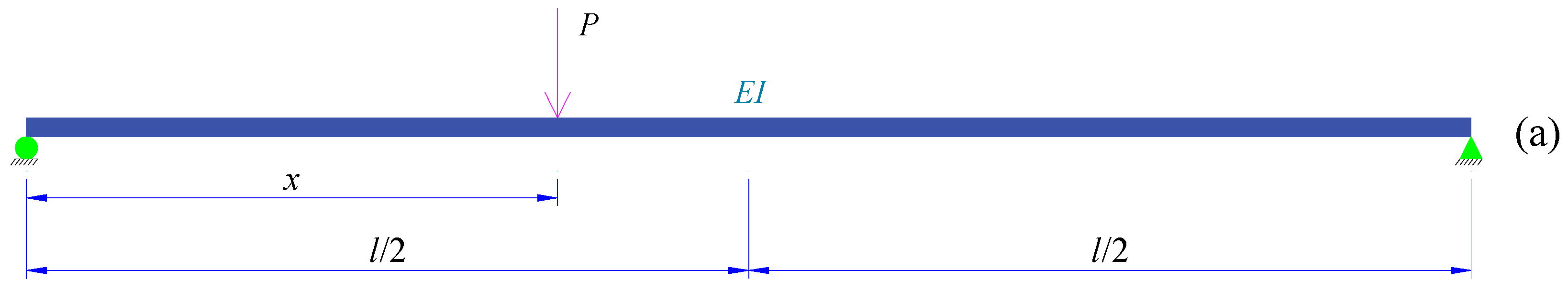
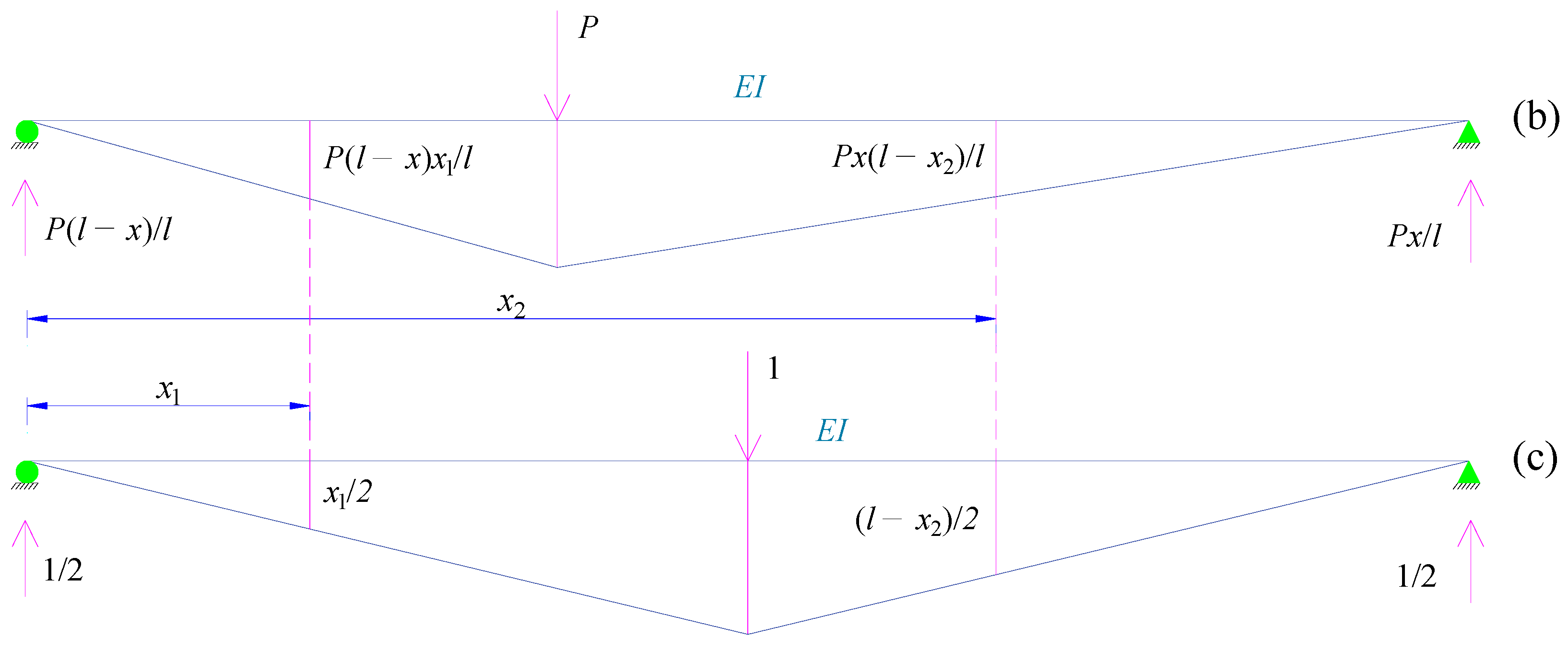
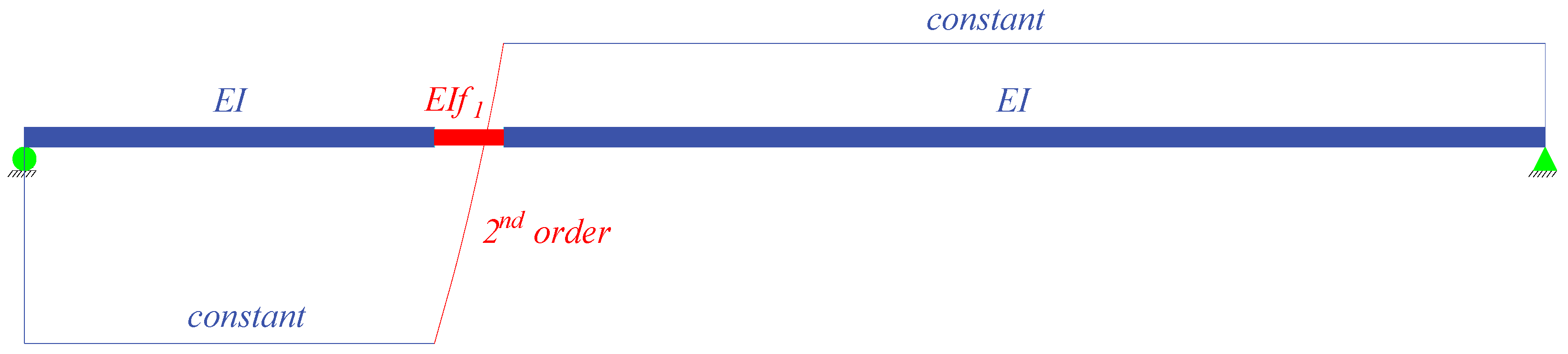
2.1. Mid-Span Deflection of the Simply Supported Beam with a Single Damaged Location

An intact SS beam with the constant bending stiffness EI under a point load P at coordinate x is considered, as depicted in Figure 1a. The deflection of the mid-span point is calculated using the following equation based on the Virtual Work principle [21,35]:

$$y^{\mathrm{intact}}={\displaystyle \underset{0}{\overset{l}{\int }}\frac{M\left(x_1\right)m\left(x_1\right)}{EI}d{x}_1}$$

(1)

where y^intact represents mid-span deflection; M(x₁) is the bending moment of the beam under point load P; m(x₁) is the bending moment of the beam subjected to the virtual unit point load at point x₁; and l is the beam length. The diagrams of M(x₁) and m(x₁) are presented in Figure 1b and Figure 1c, respectively.

By applying the boundary conditions of the beam and the formulas of M(x₁) and m(x₁) into Equation (1), the deflection of the mid-span point of the intact beam is given as follows in Equation (2):

$$y^{\mathrm{intact}}=\frac{P}{48EI}\times \{\begin{array}{ll}\left(4x^3-3x{l}^2\right)\hfill & \mathrm{if}x\le \frac{l}{2}\hfill \\ \left[4{\left(l-x\right)}^3-3\left(l-x\right)l^2\right]\hfill & \mathrm{if}x>\frac{l}{2}\hfill \end{array}$$

(2)

After establishing the formula of deflection at the mid-span point of an intact beam, the SS beam with a single-damage zone is then considered. It is assumed that the damaged zone, with a width of b, is distributed in the range [a; (a + b)] as shown in Figure 2. The damage zone has a constant bending stiffness of EIf₁, where f₁ refers to the remaining stiffness of the beam (0 ≤ f₁ ≤ 1). Three possible cases of damage locations on the SS beam are illustrated in Figure 2. Similar to the case of an intact SS beam, the mid-span deflection of the damaged beam under the point load P at position x can be calculated using Equation (3):

$$\begin{array}{l}{y}^{\mathrm{damage}1}={\displaystyle \underset{0}{\overset{a}{\int }}\frac{M\left(x_1\right)m\left(x_1\right)}{EI}d{x}_1}+{\displaystyle \underset{a}{\overset{a+b}{\int }}\frac{M\left(x_1\right)m\left(x_1\right)}{EI{f}_1}d{x}_1}+{\displaystyle \underset{a+b}{\overset{l}{\int }}\frac{M\left(x_1\right)m\left(x_1\right)}{EI}d{x}_1}\\ \hspace{0.17em}\hspace{0.17em}\hspace{0.17em}\hspace{0.17em}\hspace{0.17em}\hspace{0.17em}\hspace{0.17em}\hspace{0.17em}\hspace{0.17em}\hspace{0.17em}={\displaystyle \underset{0}{\overset{l}{\int }}\frac{M\left(x_1\right)m\left(x_1\right)}{EI}d{x}_1}+{\displaystyle \underset{a}{\overset{a+b}{\int }}\frac{1-f_1}{f_1}\frac{M\left(x_1\right)m\left(x_1\right)}{EI}d{x}_1}\\ \hspace{0.17em}\hspace{0.17em}\hspace{0.17em}\hspace{0.17em}\hspace{0.17em}\hspace{0.17em}\hspace{0.17em}\hspace{0.17em}\hspace{0.17em}\hspace{0.17em}=y^{\mathrm{intact}}+{\displaystyle \underset{a}{\overset{a+b}{\int }}\frac{1-f_1}{f_1}\frac{M\left(x_1\right)m\left(x_1\right)}{EI}d{x}_1}\end{array}$$

(3)

where y^damage1 represents the mid-span deflection of the beam with a single-damage zone. The deflection change (DC) Δy¹⁰ between the beam with a single-damage zone and the intact SS beam is then determined using Equation (4):

$$\mathsf{\Delta }{y}^{10}=y^{\mathrm{damage}1}-y^{\mathrm{intact}}={\displaystyle \underset{a}{\overset{a+b}{\int }}\frac{1-f_1}{f_1}\frac{M\left(x_1\right)m\left(x_1\right)}{EI}d{x}_1}$$

(4)

The integral in Equation (4) is then calculated as follows in Equations (5)–(7):

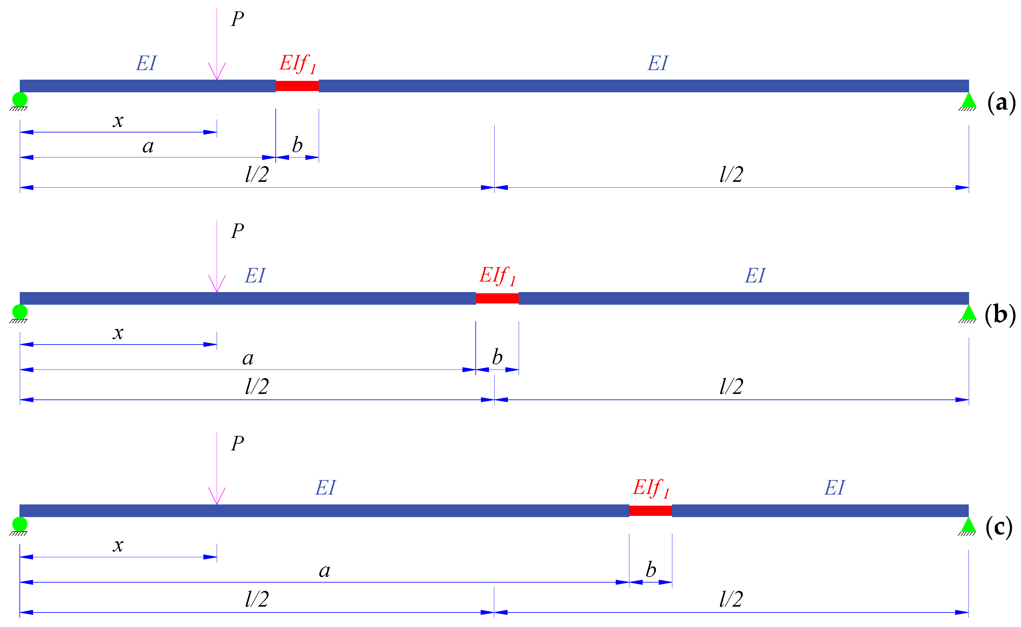
• The damage zone is located on the left-half beam:

$$\mathsf{\Delta }{y}^{10}=\frac{P}{ EI}\frac{\left(1-f_1\right)}{f_1}\times \{\begin{array}{ll}\frac{b\left(6a^2+6ab+2b^2-6la-3lb\right)}{12l}x\hfill & \mathrm{if}0\le x<a\hfill \\ \frac{\left[2l{a}^3+\left(6a^{2}b+6a{b}^2+2b^3-3l{\left(a+b\right)}^2\right)x+l{x}^3\right]}{12l}\hfill & \mathrm{if}a\le x<\left(a+b\right)\hfill \\ -\frac{b\left(3a^2+3ab+b^2\right)}{6l}\left(l-x\right)\hfill & \mathrm{if}\left(a+b\right)\le x\hfill \end{array}$$

(5)

• The damage zone is located at the mid-span point:

$$\mathsf{\Delta }{y}^{10}=\frac{P}{ EI}\frac{\left(1-f_1\right)}{f_1}\times \{\begin{array}{ll}-\frac{\left(8{\left(a+b-l\right)}^3+8a^3-12a^{2}l+3l^3\right)}{48l}x\hfill & \mathrm{if}0\le x<a\hfill \\ \left[\frac{4l{x}^3-\left(8{\left(a+b-l\right)}^3+8a^3+3l^3\right)x+8a^{3}l}{48l}\right]\hfill & \mathrm{if}a\le x<\frac{l}{2}\hfill \\ \left[\frac{4l{\left(l-x\right)}^3-8x{\left(a+b-l\right)}^3-8x{a}^3-3l^3\left(l-x\right)+8a^{3}l}{48l}\right]\hfill & \mathrm{if}\frac{l}{2}\le x<\left(a+b\right)\hfill \\ \frac{\left[8{\left(a+b\right)}^3-12l{\left(a+b\right)}^2+8a^3+l^3\right]}{48l}\left(l-x\right)\hfill & \mathrm{if}x>\left(a+b\right)\hfill \end{array}$$

(6)

• The damage zone is located on the right-half beam:

$$\mathsf{\Delta }{y}^{10}=\frac{P}{ EI}\frac{\left(1-f_1\right)}{f_1}\times \{\begin{array}{ll}-\frac{b \left(3a^2+3ab-6al+b^2-3bl+3l^2\right)}{6 l}x\hfill & \mathrm{if}x<a\hfill \\ -\frac{\left[\begin{array}{l}l{x}^3-3l^2{x}^2+a^{2}l\left(2a-3l\right)\\ +\left(2{\left(a+b-l\right)}^3-2a^3+3a^{2}l+2l^3\right)x\end{array}\right]}{12 l}\hfill & \mathrm{if}a\le x<\left(a+b\right)\hfill \\ \frac{b \left(6a^2+6ab+2b^2-6la-3lb\right)}{12l}\left(l-x\right)\hfill & \mathrm{if}x\ge \left(a+b\right)\hfill \end{array}$$

(7)

For simplicity, Equations (5)–(7) are condensed as Equation (8):

$$\mathsf{\Delta }{y}^{10}=\frac{P}{ EI}\times \frac{\left(1-f_1\right)}{f_1}\times [\begin{array}{ll}{g}^3\left(x\right)\hfill & \mathrm{in}\mathrm{the}\mathrm{damage}\mathrm{zone}\hfill \\ h^1\left(x\right)\hfill & \mathrm{outside}\mathrm{the}\mathrm{damage}\mathrm{zone}\hfill \end{array}$$

(8)

where h¹(x) and g³(x) are linear and cubic functions of x, respectively. These functions depend only on the parameters a, b, and l, as shown in Equations (5)–(7). Figure 3 shows the value of Δy¹⁰ when the applied load P is “moving” on the beam. As depicted, the mid-span deflection change equals zero at the two bearings, rises progressively as it approaches the damage zone, and reaches its maximum value in this zone. Therefore, the damage zone can be approximated around the extreme point of deflection change, Δy¹⁰, or near the point where two deflection change lines converge. Furthermore, Figure 3 illustrates how the interval boundaries between the cubic function and two linear functions can be used to identify the damage zone more accurately.

In addition, the first and second derivatives of DC (details are shown in the Appendix A) are obtained using Equations (9) and (10):

$$\frac{\partial \mathsf{\Delta }{y}^{10}}{\partial x}=\frac{P}{ EI}\times \frac{\left(1-f_1\right)}{f_1}\times [\begin{array}{ll}{g}^2\left(x\right)\hfill & \mathrm{in}\mathrm{the}\mathrm{damage}\mathrm{zone}\hfill \\ \mathrm{constant}\hfill & \mathrm{outside}\mathrm{the}\mathrm{damage}\mathrm{zone}\hfill \end{array}$$

(9)

$$\frac{{\partial }^2\mathsf{\Delta }{y}^{10}}{\partial x^2}=\frac{P}{ EI}\times \frac{\left(1-f_1\right)}{f_1}\times [\begin{array}{ll}{g}^1\left(x\right)\hfill & \mathrm{in}\mathrm{the}\mathrm{damage}\mathrm{zone}\hfill \\ 0\hfill & \mathrm{outside}\mathrm{the}\mathrm{damage}\mathrm{zone}\hfill \end{array}$$

(10)

where g¹(x) and g²(x) are the linear and quadratic functions of x, respectively. The first- and second derivatives of DC are illustrated in Figure 4 and Figure 5. As depicted in Figure 4, the first derivative of DC is a quadratic curve in the damage zone that takes constant values on the left and right sides of this zone. In the damage zone, the second derivative of DC provides non-zero values (a linear function), but provides zero elsewhere, as shown in Figure 5. These are also important indicators for identifying the location of the damage zones.

2.2. Damage Index

If f₁ represents the remaining stiffness of the SS beam, the damage severity coefficient is (1 − f₁). Thus, the damage index can be defined as β = (1 − f₁)/f₁. This damage index is easily determined using Equations (8)–(10) if the damage location, the stiffness EI, and the load P are known. However, in reality, beam stiffness is often unknown or not precisely determined, especially for the structure in use. Therefore, it is necessary to find a method to determine the damage index β when the stiffness EI is unknown and when the applied load P is not constant. Equations (2), (8)–(10) can be written as Equations (11)–(14) as follows:

$$y^{\mathrm{intact}}=\frac{P}{EI}\times k^3\left(x\right)$$

(11)

$$\mathsf{\Delta }{y}^{10}=\frac{P}{ EI}\times \beta \times [\begin{array}{ll}{g}^3\left(x\right)\hfill & \mathrm{in}\mathrm{the}\mathrm{damage}\mathrm{zone}\hfill \\ h^1\left(x\right)\hfill & \mathrm{outside}\mathrm{the}\mathrm{damage}\mathrm{zone}\hfill \end{array}$$

(12)

$$\frac{\partial \mathsf{\Delta }{y}^{10}}{\partial x}=\frac{P}{ EI}\times \beta \times [\begin{array}{ll}{g}^2\left(x\right)\hfill & \mathrm{in}\mathrm{the}\mathrm{damage}\mathrm{zone}\hfill \\ \mathrm{constant}\hfill & \mathrm{outside}\mathrm{the}\mathrm{damage}\mathrm{zone}\hfill \end{array}$$

(13)

$$\frac{{\partial }^2\mathsf{\Delta }{y}^{10}}{\partial x^2}=\frac{P}{ EI}\times \beta \times [\begin{array}{ll}{g}^1\left(x\right)\hfill & \mathrm{in}\mathrm{the}\mathrm{damage}\mathrm{zone}\hfill \\ 0\hfill & \mathrm{outside}\mathrm{the}\mathrm{damage}\mathrm{zone}\hfill \end{array}$$

(14)

where k³(x) is the cubic function of x. As seen in these equations, P/EI can be eliminated by dividing both sides of Equations (12)–(14) by Equation (11) leading to Equations (15)–(17). This allows for the determination of the damage index as well as the remaining stiffness.

$$\frac{\mathsf{\Delta }{y}^{10}}{y^{\mathrm{intact}}}=\frac{\beta }{ k^3\left(x\right)}\times [\begin{array}{ll}{g}^3\left(x\right)\hfill & \mathrm{in}\mathrm{the}\mathrm{damage}\mathrm{zone}\hfill \\ h^1\left(x\right)\hfill & \mathrm{outside}\mathrm{the}\mathrm{damage}\mathrm{zone}\hfill \end{array}$$

(15)

$$\frac{\partial \mathsf{\Delta }{y}^{10}}{\partial x}\times \frac{1}{y^{\mathrm{intact}}}=\frac{\beta }{ k^3\left(x\right)}\times [\begin{array}{ll}{g}^2\left(x\right)\hfill & \mathrm{in}\mathrm{the}\mathrm{damage}\mathrm{zone}\hfill \\ \mathrm{constant}\hfill & \mathrm{outside}\mathrm{the}\mathrm{damage}\mathrm{zone}\hfill \end{array}$$

(16)

$$\frac{{\partial }^2\mathsf{\Delta }{y}^{10}}{\partial x^2}\times \frac{1}{y^{\mathrm{intact}}}=\frac{\beta }{ k^3\left(x\right)}\times [\begin{array}{ll}{g}^1\left(x\right)\hfill & \mathrm{in}\mathrm{the}\mathrm{damage}\mathrm{zone}\hfill \\ 0\hfill & \mathrm{outside}\mathrm{the}\mathrm{damage}\mathrm{zone}\hfill \end{array}$$

(17)

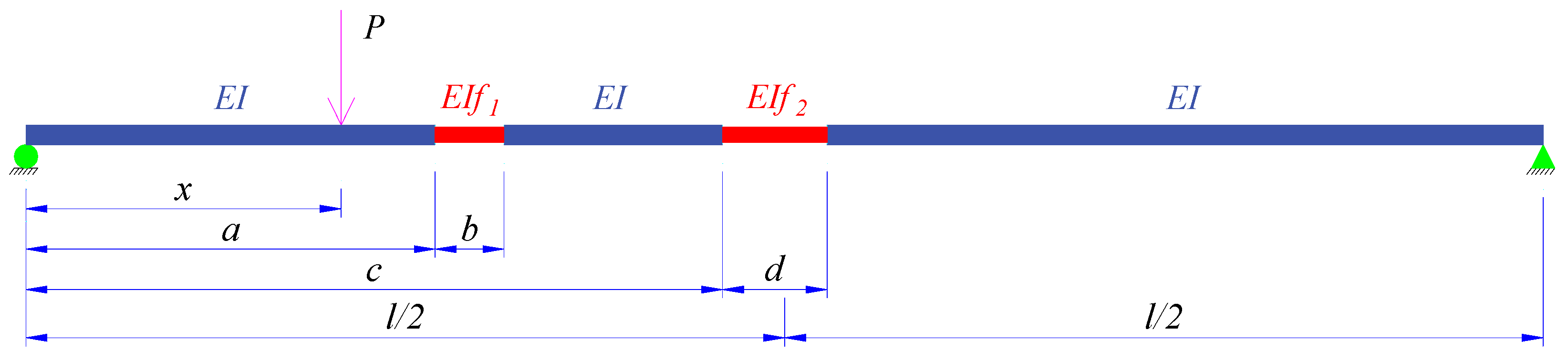
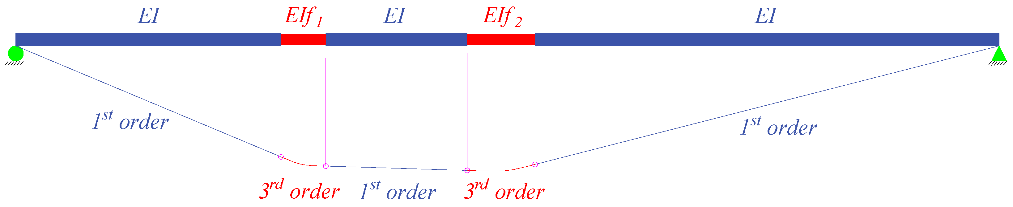
2.3. Mid-Span Deflection of the Simply Supported Beam with Two Damaged Locations

In the second case study, let us assume that there is an SS beam with two damage zones, as depicted in Figure 6. The first damage zone mirrors the information from the first case study. For the second damage zone, positioned at c from the left bearing, a width of d is considered. This second damage zone maintains a constant bending stiffness of EIf₂, where f₂ represents the remaining beam stiffness within this zone. Mid-span deflection can be represented as follows:

$$\begin{array}{l}{y}^{\mathrm{damage}2}={\displaystyle \underset{0}{\overset{a}{\int }}\frac{M\left(x_1\right)m\left(x_1\right)}{EI}d{x}_1}+{\displaystyle \underset{a}{\overset{a+b}{\int }}\frac{M\left(x_1\right)m\left(x_1\right)}{EI{f}_1}d{x}_1}+{\displaystyle \underset{a+b}{\overset{c}{\int }}\frac{M\left(x_1\right)m\left(x_1\right)}{EI}d{x}_1}\\ +{\displaystyle \underset{c}{\overset{c+d}{\int }}\frac{M\left(x_1\right)m\left(x_1\right)}{EI{f}_2}d{x}_1}+{\displaystyle \underset{c+d}{\overset{l}{\int }}\frac{M\left(x_1\right)m\left(x_1\right)}{EI}d{x}_1}\\ ={\displaystyle \underset{0}{\overset{a}{\int }}\frac{M\left(x_1\right)m\left(x_1\right)}{EI}d{x}_1}+{\displaystyle \underset{a}{\overset{a+b}{\int }}\frac{M\left(x_1\right)m\left(x_1\right)}{EI{f}_1}d{x}_1}+{\displaystyle \underset{a+b}{\overset{l}{\int }}\frac{M\left(x_1\right)m\left(x_1\right)}{EI}d{x}_1}\\ +{\displaystyle \underset{c}{\overset{c+d}{\int }}\frac{1-f_2}{f_2}\frac{M\left(x_1\right)m\left(x_1\right)}{EI}d{x}_1}\end{array}$$

(18)

where y^damage2 is the mid-span deflection of the beam with two damage zones. Equation (18) can be re-expressed using Equation (19) via combination with Equation (3):

$$y^{\mathrm{damage}2}=y^{\mathrm{damage}1}+{\displaystyle \underset{c}{\overset{c+d}{\int }}\frac{1-f_2}{f_2}\frac{M\left(x_1\right)m\left(x_1\right)}{EI}d{x}_1}$$

(19)

Therefore, the DC from one damage area to two damage zones can be written as shown in Equation (20):

$$\mathsf{\Delta }{y}^{21}=y^{\mathrm{damage}2}-y^{\mathrm{damage}1}={\displaystyle \underset{c}{\overset{c+d}{\int }}\frac{1-f_2}{f_2}\frac{M\left(x_1\right)m\left(x_1\right)}{EI}d{x}_1}$$

(20)

Similar to the first case study in Section 2.1, it is possible to determine the location of the damage in this scenario. The results remain the same as those in Equations (5)–(7), except that the three parameters a, b, and f₁ are replaced by c, d, and f₂, respectively.

The DC in this scenario can be expressed as the cubic function in the second damage zone, as shown in Figure 7, and as the linear function in the remaining zone, analogous to the description in Section 2.1. Consequently, the determination of the position of the second damage can also be performed as explained in Section 2.1. The DC in the scenario from the intact beam to the beam with two damage zones can be expressed as shown in Figure 8 and Equation (21):

$$\mathsf{\Delta }{y}^{20}=y^{\mathrm{damage}2}-y^{\mathrm{intact}}=\left(y^{\mathrm{damage}2}-y^{\mathrm{damage}1}\right)+\left(y^{\mathrm{damage}1}-y^{\mathrm{intact}}\right)=\mathsf{\Delta }{y}^{21}+\mathsf{\Delta }{y}^{10}$$

(21)

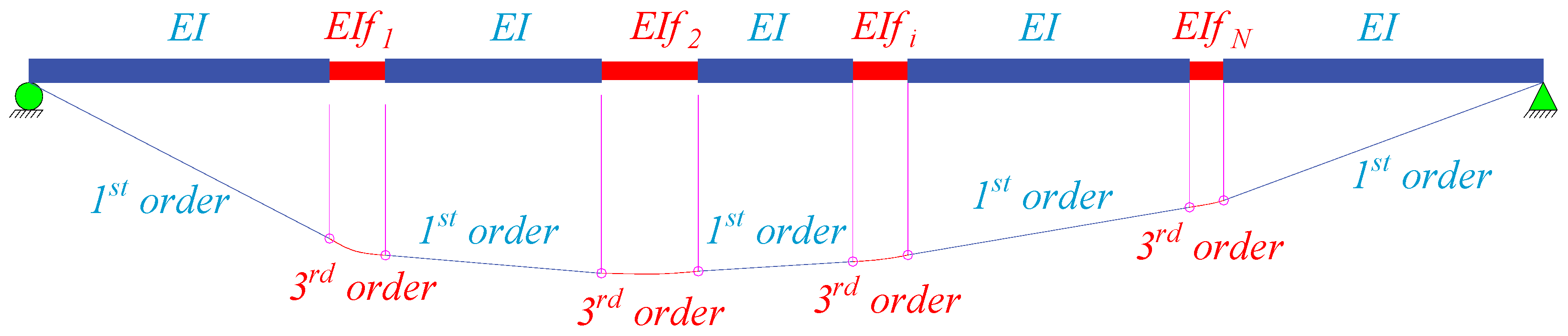
2.4. Mid-Span Deflection of the Simply Supported Beam with Many Damaged Locations

Using this characteristic, the calculation for an SS beam with an N damage zones follows the same procedure outlined in Section 2.3, utilizing Equation (22):

$$\mathsf{\Delta }{y}^{N0}={\displaystyle \sum _N^1\mathsf{\Delta }{y}^{i\left(i-1)\right)}}=\mathsf{\Delta }{y}^{N\left(N-1\right)}+\dots +\mathsf{\Delta }{y}^{21}+\mathsf{\Delta }{y}^{10}$$

(22)

The pattern of the Δy^N0 diagram can be discerned from the Δyⁱ⁽ⁱ⁻¹⁾ diagrams. Similar to the Δy²¹ diagram presented in Section 2.3, the Δyⁱ⁽ⁱ⁻¹⁾ diagram comprises two components: there is (1) a cubic line within the ith damage zone and there are (2) straight lines in the remaining zones. It should be noted that combining two straight lines results in another straight line while adding a straight line to a cubic curve will yield a cubic curve. Consequently, the Δy^N0 diagram features cubic curves at N damage zones and straight lines in the remaining zones, as depicted in Figure 9.

2.5. The Proposed Framework of Identification of Damage Zones in SS Beam

Assuming that the first structural state is known, the proposed method outlined above facilitates the identification of new existing damage zones from this state until the second structural state. The procedure entails the following:

• Step 1: Calculate y^N, representing the mid-span deflection at the second structural state, by applying a static load P at various positions along the beam.
• Step 2: Determine Δy^N0 = y^N − y⁰ where y⁰ denotes the mid-span deflection at the first structural state.
• Step 3: Plot the Δy^N0 diagram.
• Step 4: Identify the new damage zones following these fundamental principles:

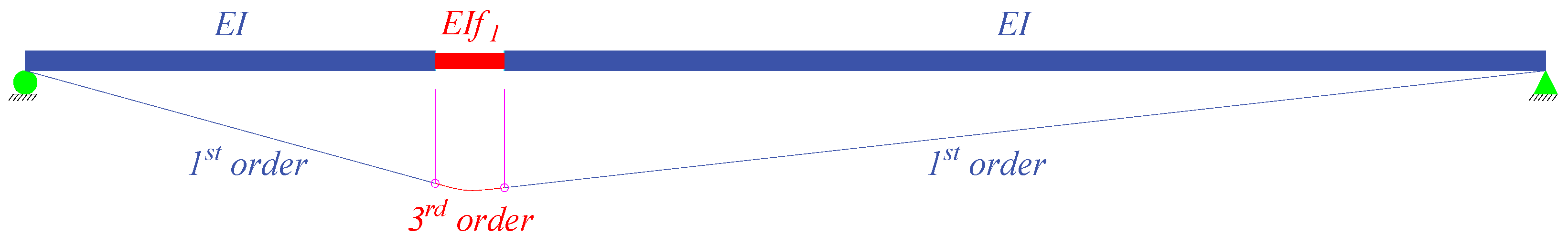
• New damage zones exhibit cubic curve shapes, while the remaining zones display straight-line shapes.
• New damaged positions are typically found near the intersection of two consecutive first-order lines on the diagram, and new damage zones are discerned through the two consecutive intersection points between the first-order line and the cubic curve.
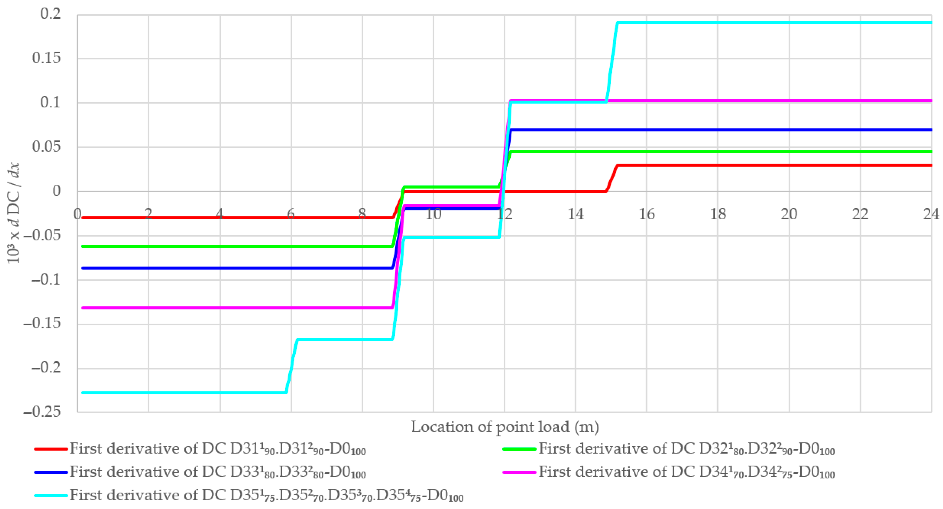
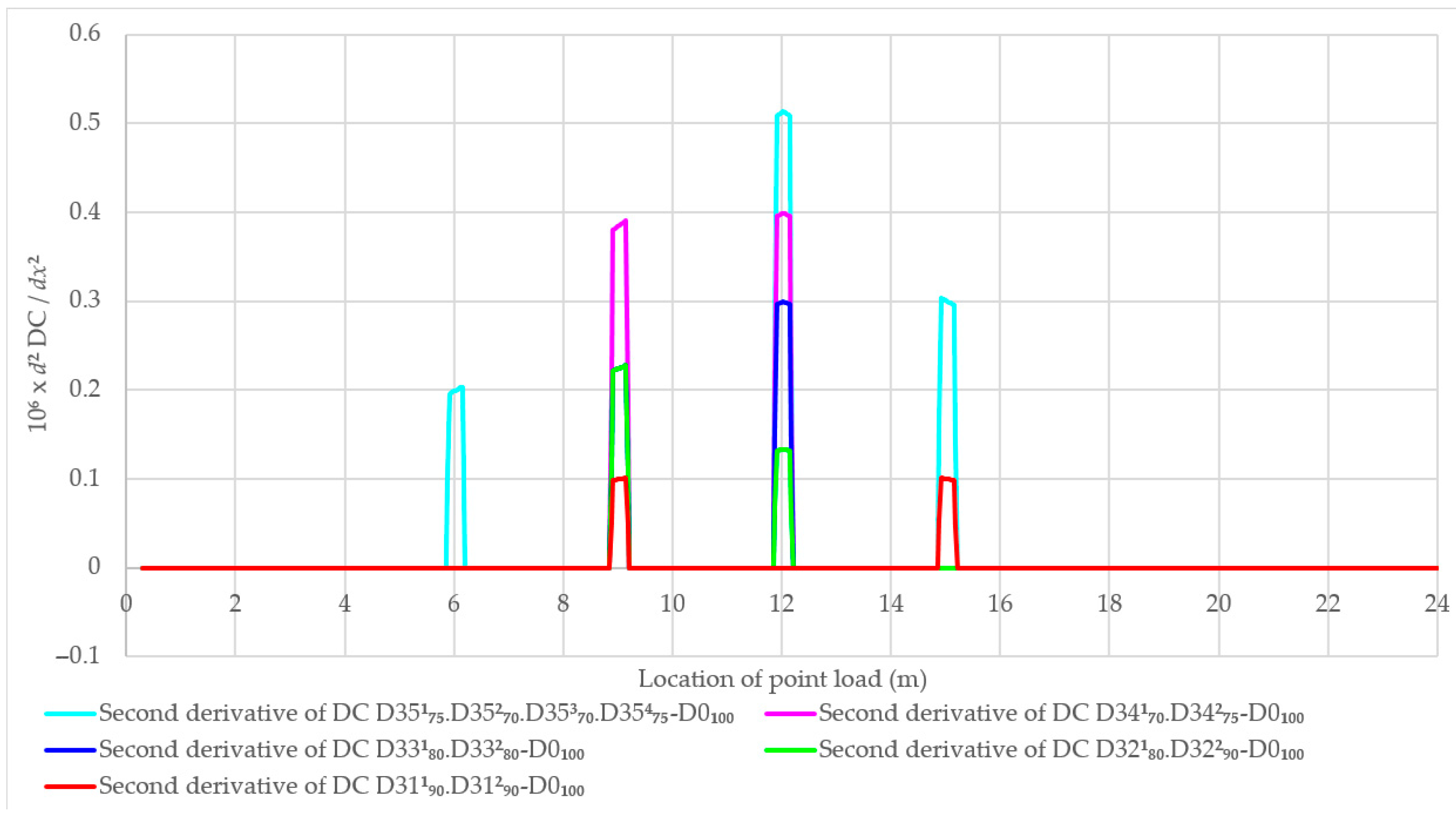
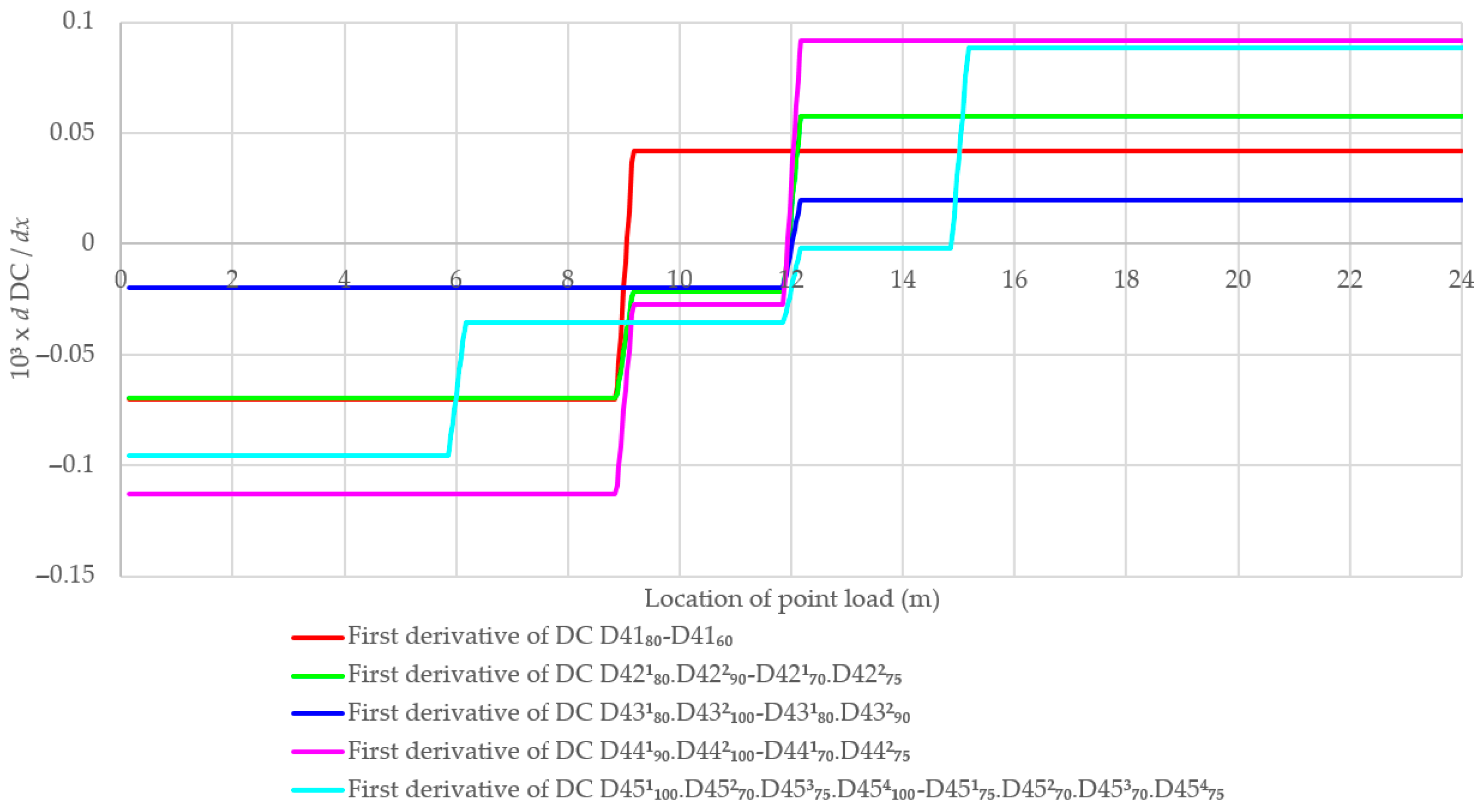
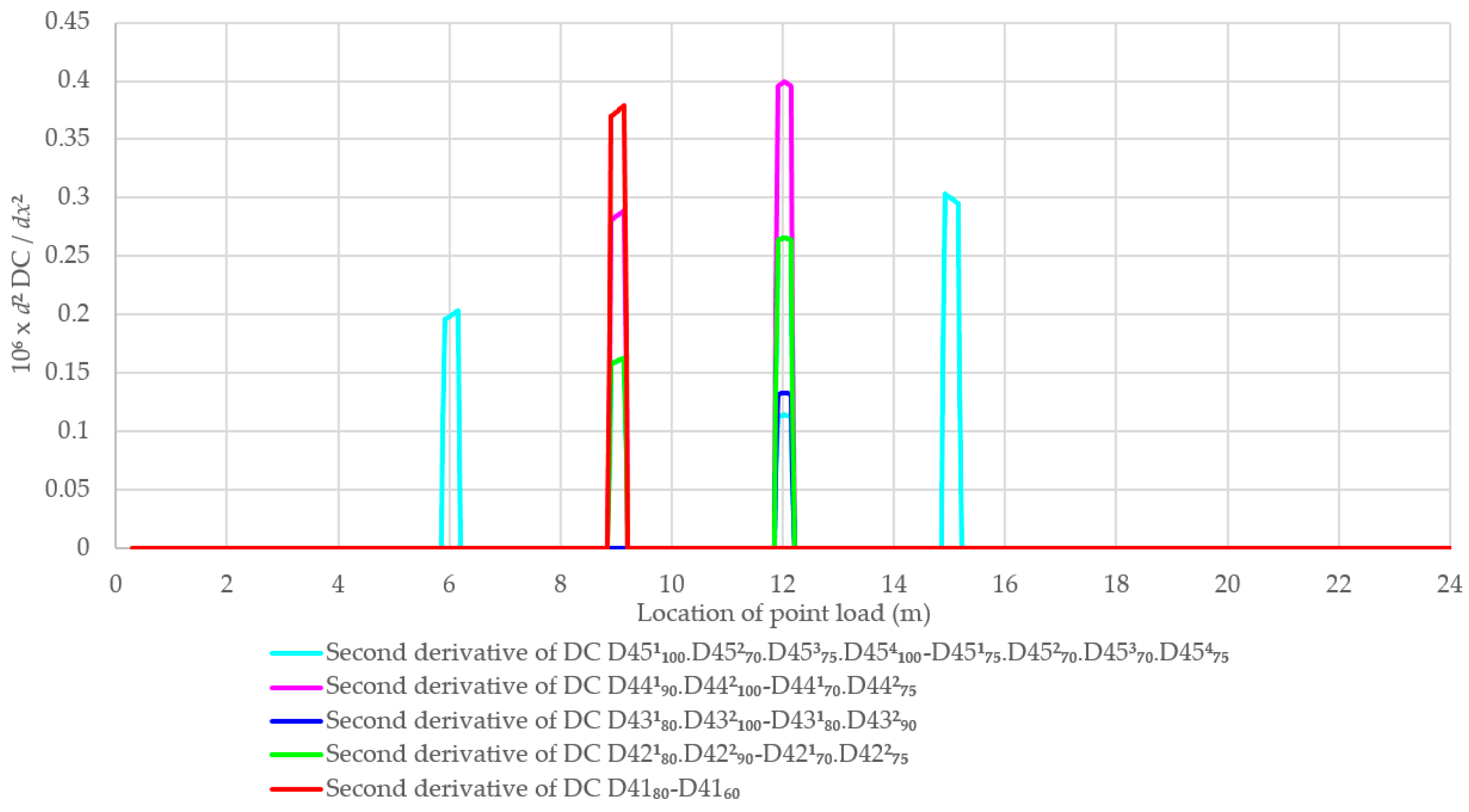
• The first and second derivatives of DC can also aid in determining the damage location and the damage index.

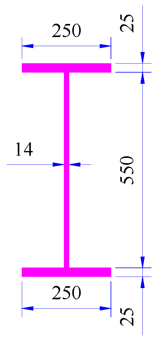
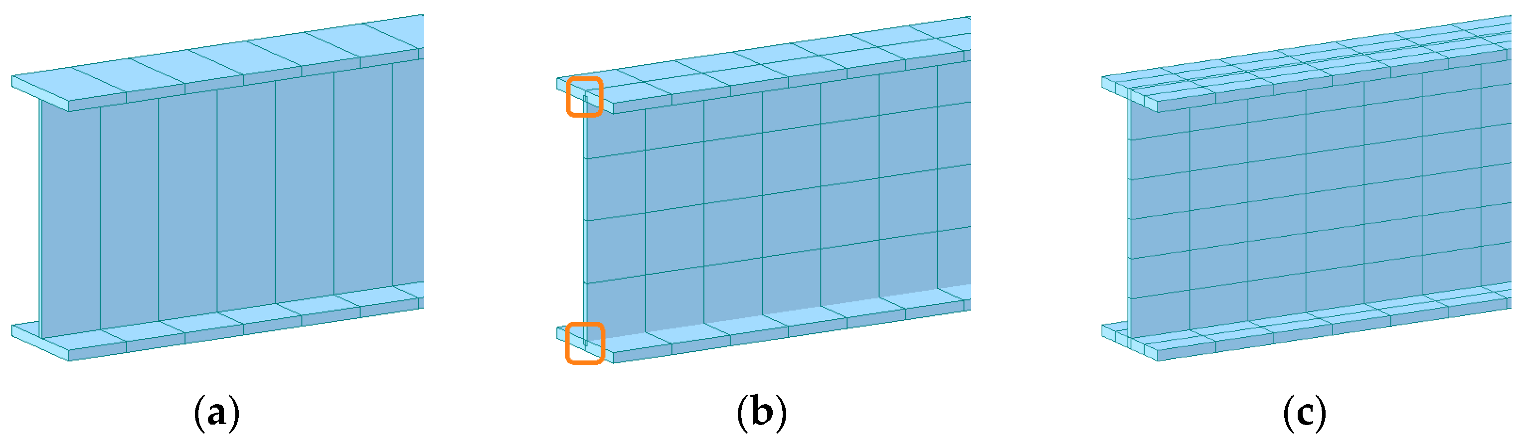
3. Description of Case Studies

In this study, an SS beam with a length of 24,000 mm is considered. The two supports (bearings) are positioned at the beam’s ends. The beam’s cross-section is a wide flange section comprising a compression flange and a tension flange of 250 × 25 mm, along with a web of 550 × 14 mm, as illustrated in Figure 10. The Poisson’s ratio is set at 0.3 and the density of steel is 7850 kg/m³. Additionally, the elastic modulus of steel is 200 GPa. To estimate the beam responses, a static point load P of 5 tons (49.05 kN) is applied in a downward direction at various points along the beam. Three numerical models, implemented in Midas FEA NX 2020 (v1.1) software [36], are employed to validate the proposed theoretical method. The first model utilizes beam elements to describe the I-beam, the next model employs plate elements to describe the compression flange, tension flange, and beam web, and the final model uses solid elements to describe the I-beam, as depicted in Figure 11. Unlike the proposed theoretical method, these numerical models apply the Timoshenko–Ehrenfest beam theory, which converges towards the Euler–Bernoulli beam theory. Figure 12 illustrates the mid-span deflection curves in the intact SS beam obtained by using the proposed method with Equation (2) and numerical models.

As evident from the figure, the curves derived from both the theoretical and numerical methods exhibit minimal discrepancies. The mid-span deflection values obtained from the proposed method and the numerical models, using beam, plate, and solid elements, are as follows: −57.9364 mm, −56.7014 mm, −57.9528 mm, and −57.5064 mm, respectively. The lowest deflection result from the plate element is attributed to material superposition between the compression flange–beam web and the tension flange–beam web, as indicated in the orange section in Figure 11b. In this scenario, a portion of the beam web is calculated twice on the two flanges, increasing beam stiffness and consequently resulting in a significant decrease in deflection. For the remaining three models, the deflection of the proposed model is approximately 0.74% to 0.77% lower than that of the beam and solid models, respectively. This variance arises from the inherent assumptions of the Timoshenko–Ehrenfest beam theory compared to the Euler–Bernoulli beam theory. Subsequently, several case studies of the damaged beam are considered using the following information, while the results and discussions are presented in Section 4. The deflection values of the finite element (FE) beam and FE solid models are nearly identical. Consequently, the subsequent sections will employ the FE beam model as the numerical representation.

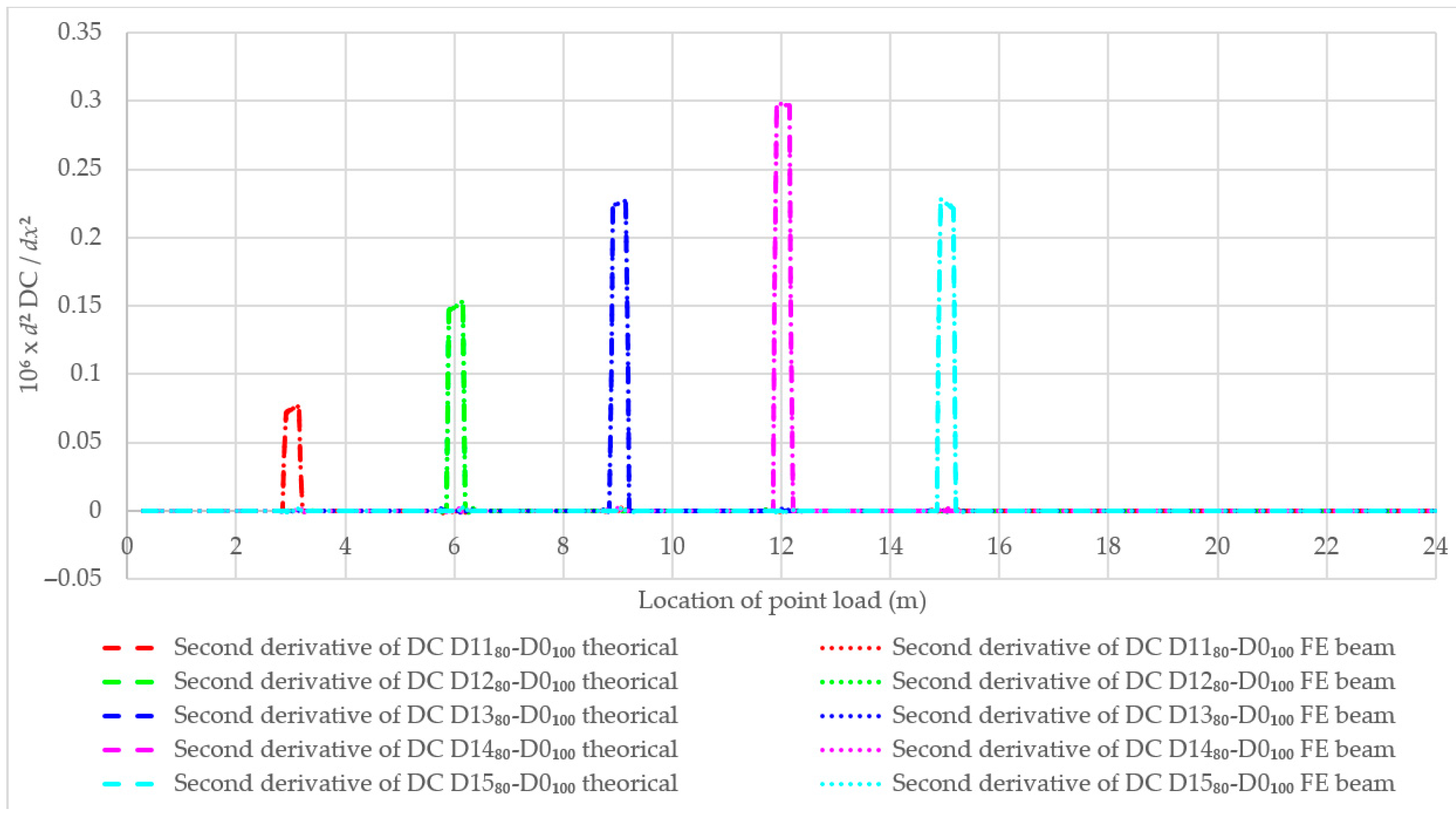
3.1. Single-Damage Beams with Different Positions and the Same Remaining Stiffness

The first case study examines a beam with a single-damage zone at various positions along its length. Specifically, five locations are investigated, including points at 1/8, 1/4, 3/8, 1/2, and 5/8 of the beam’s length. In all cases, the remaining stiffness of the damage zone remains constant, set at 80% of the intact beam stiffness. These scenarios are summarized in

Table 1. Single-damage cases with different positions.

No	Damage Case	Damage Location	Remaining Stiffness of the Damage Zone	Remarks
1-0	D0100%			Intact beam
1-1	D1180%	2850–3150 mm	80%	One new damage zone
1-2	D1280%	5850–6150 mm	80%	One new damage zone
1-3	D1380%	8850–9150 mm	80%	One new damage zone
1-4	D1480%	11,850–12,150 mm	80%	One new damage zone
1-5	D1580%	14,850–15,150 mm	80%	One new damage zone

.

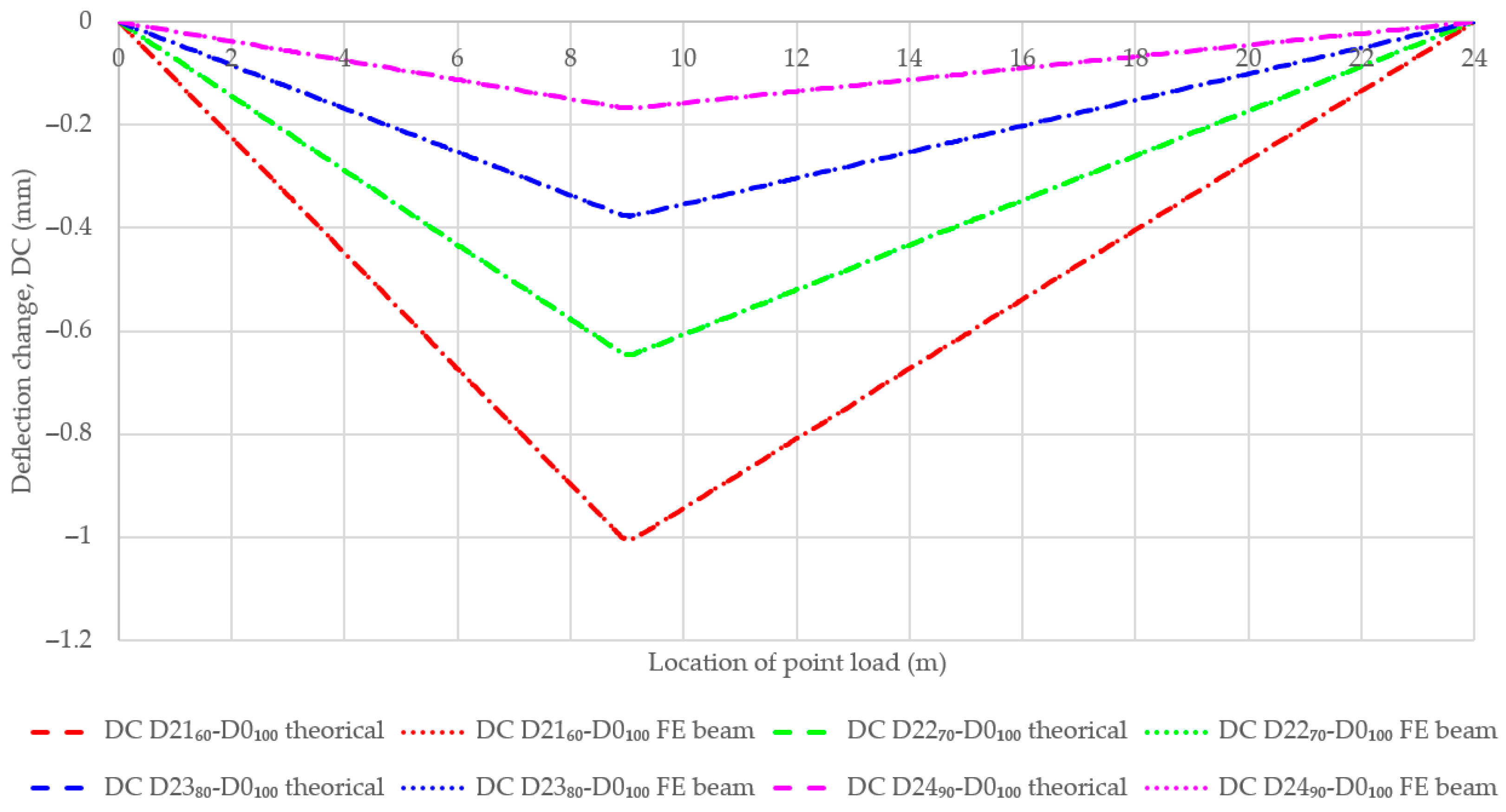
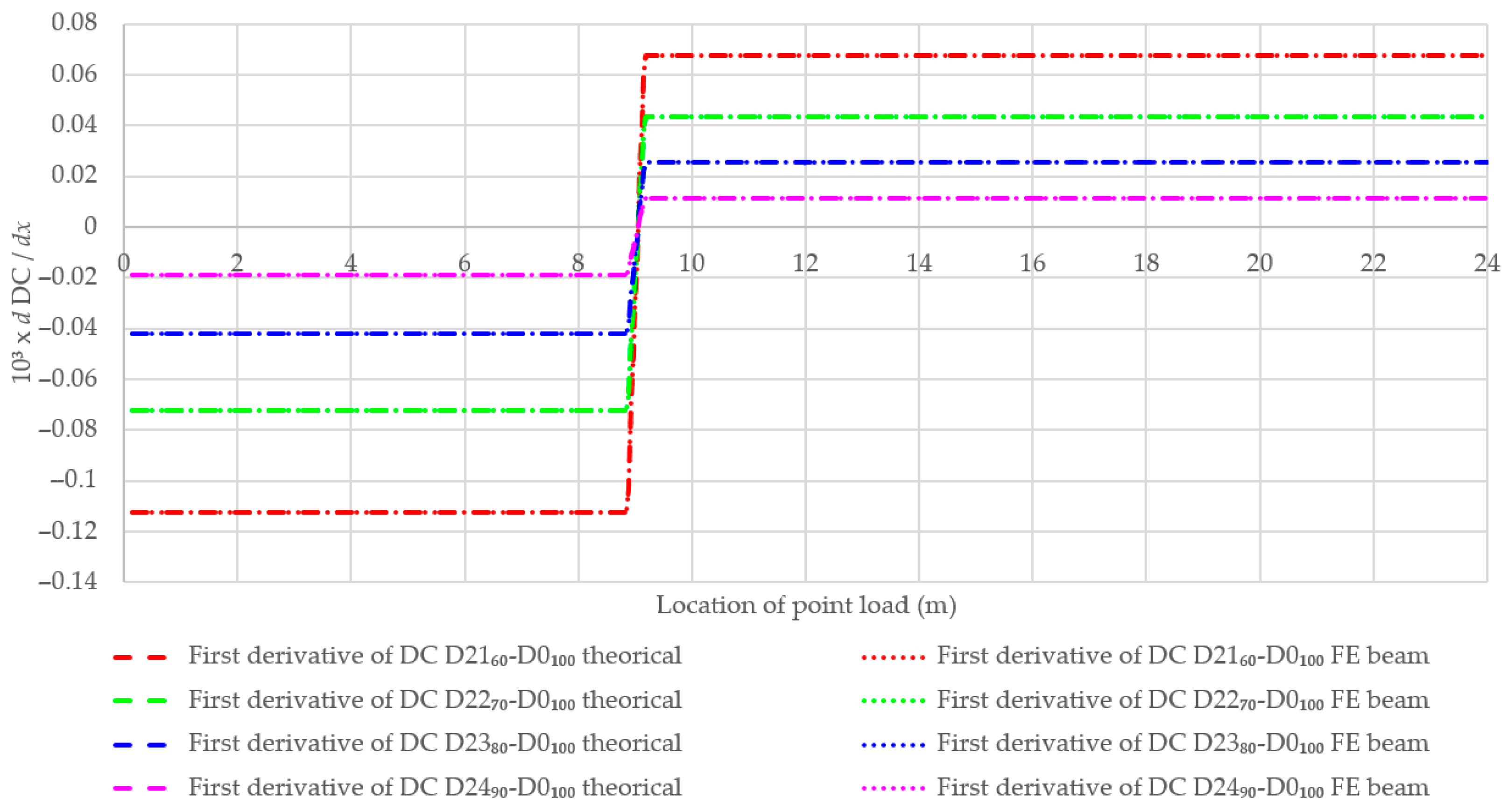
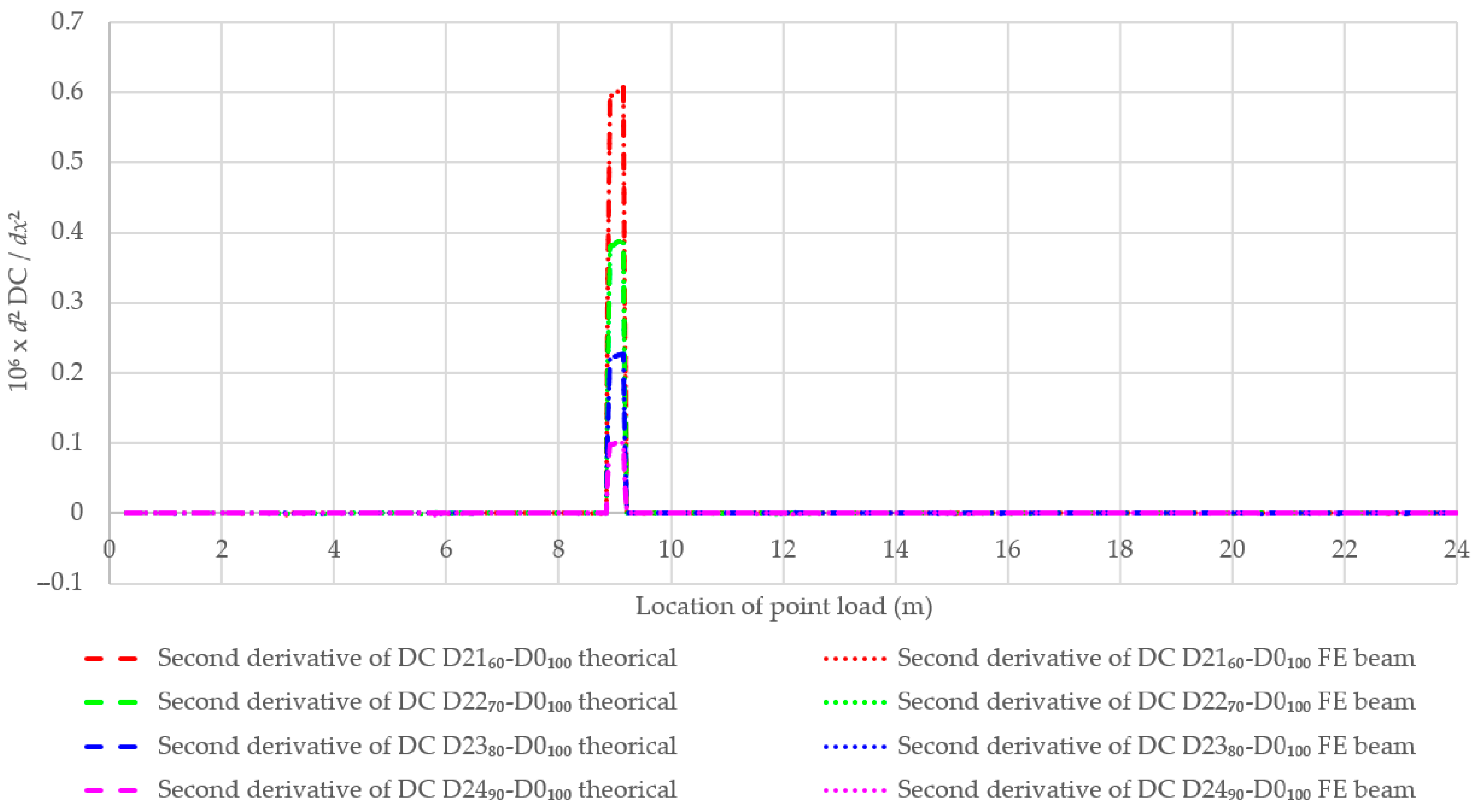
3.2. Single-Damage Beam at the Same Positions with Different Remaining Stiffness

This case study focuses on a beam with a single-damage zone fixed at the 3/8 point of the beam’s length. However, the remaining stiffness of the damage zone varies across cases, ranging from 60% to 90% of the intact beam’s stiffness. Details of these cases are provided in

Table 2. Single-damage cases with different remaining stiffness.

No	Damage Case	Damage Location	Remaining Stiffness of the Damage Zone	Remarks
2-1	D2160%	8850–9150 mm	60%	One new damage zone
2-2	D2270%	8850–9150 mm	70%	One new damage zone
2-3	D2380%	8850–9150 mm	80%	One damage zone, same case of D1380%
2-4	D2490%	8850–9150 mm	90%	One new damage zone

.

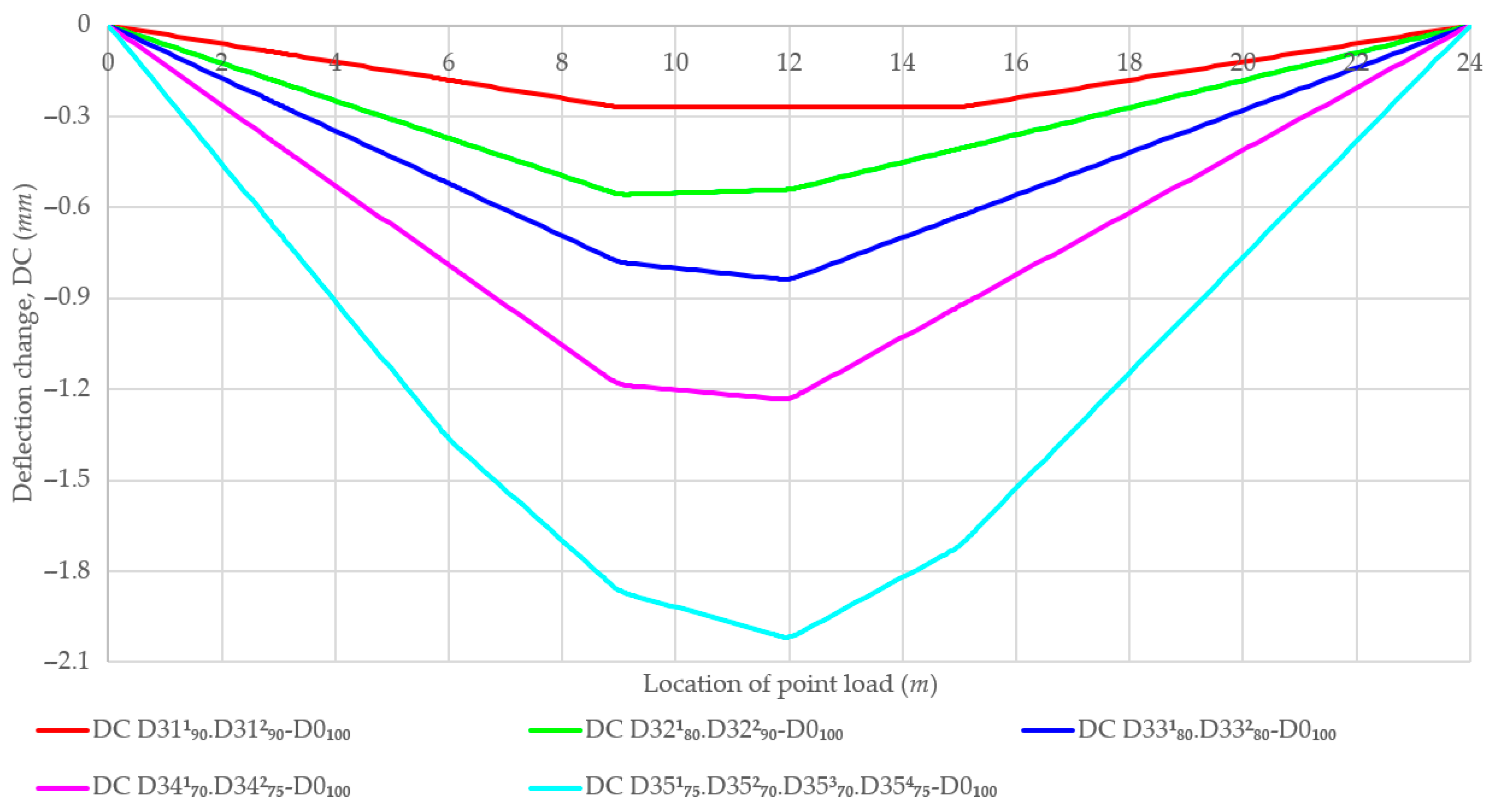
3.3. Beam with Multiple Damage Zones Compared to Intact Beam

In this case study, the effects of multiple damage zones on the mid-span deflection are taken into account by comparing them with the intact beam. Various scenarios with two and four damage zones are considered, including cases with identical and differing remaining stiffness values. These are presented in

Table 3. Multiple damage cases compared to intact beam.

No	Damage Case	Damage Location	Remaining Stiffness of the Damage Zone	Remarks
3-1	D31190%.D31290%	D311: 8850–9150 mm	90%	Two new damage zones
		D314: 14,850–15,150 mm	90%
3-2	D32180%.D32290%	D321: 8850–9150 mm	80%	Two new damage zones
		D322: 11,850–12,150 mm	90%
3-3	D33180%.D33280%	D331: 8850–9150 mm	80%	Two new damage zones
		D332: 11,850–12,150 mm	80%
3-4	D34170%.D34275%	D341: 8850–9150 mm	70%	Two new damage zones
		D342: 11,850–12,150 mm	75%
3-5	D35175%.D35270%.D35370%.D35475%	D351: 5850–6150 mm	75%	Four new damage zones
		D352: 8850–9150 mm	70%
		D353: 11,850–12,150 mm	70%
		D354: 14,850–15,150 mm	75%

.

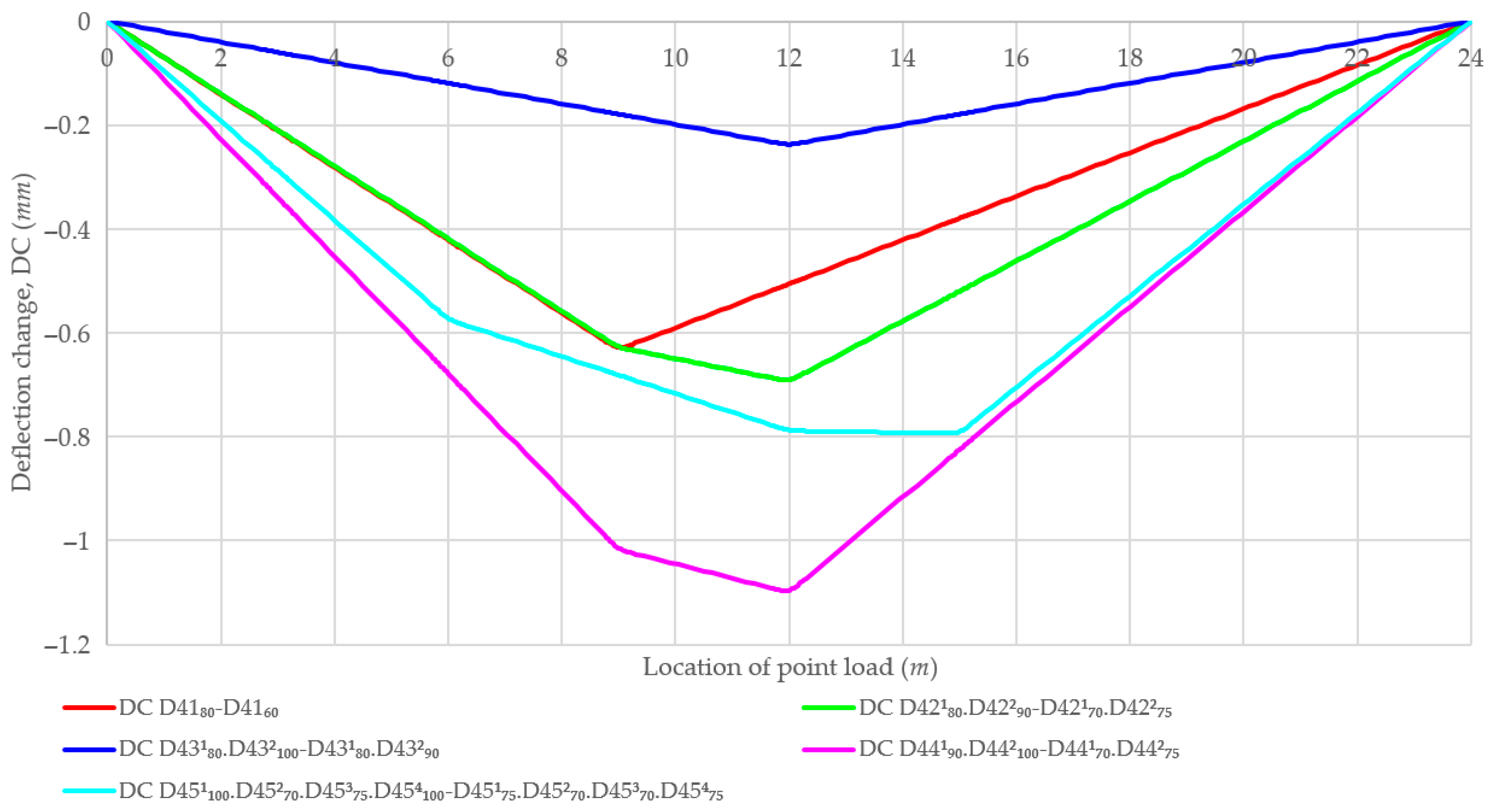
3.4. Beam with Multiple Damage Zones Considering New Damages and Development of Existing Damage

This case study extends the previous scenarios in Section 3.1, Section 3.2 and Section 3.3 to investigate the effects of developing new damage zones or the continued growth of existing ones. Five specific cases are examined, detailed in

Table 4. Multiple damage beam with new damages and development of existing damages.

No	Damage Case	Damage Location	Remaining Stiffness		Remarks
			1st Structural State	2nd Structural State
4-1	D4180% → D4160%	D41: 8850–9150 mm	80%	60%	One existing damage zone is developing.
4-2	D42180%.D42290% → D42170%.D42275%	D421: 8850–9150 mm	80%	70%	Two existing damage zones are developed simultaneously.
		D422: 11,850–12,150 mm	90%	75%
4-3	D43180%.D432100% → D43180%.D43290%	D431: 8850–9150 mm	80%	80%	The existing damage is not developed, but new damage appears.
		D432: 11,850–12,150 mm	100%	90%
4-4	D44190%.D442100% → D44170%.D44275%	D441: 8850–9150 mm	90%	70%	The existing damage is developing, while new damage appears.
		D442: 11,850–12,150 mm	100%	75%
4-5	D451100%.D45270%.D45375%.D454100% → D45175%.D45270%.D45370%.D45475%	D451: 5850–6150 mm	100%	75%	One existing damage zone is developing and one other is not, while two new damage zones appear.
		D452: 8850–9150 mm	70%	70%
		D453: 11,850–12,150 mm	75%	70%
		D454: 14,850–15,150 mm	100%	75%

. These include scenarios where existing damages continue to develop, new damage zones emerge, or a combination of both occurs.

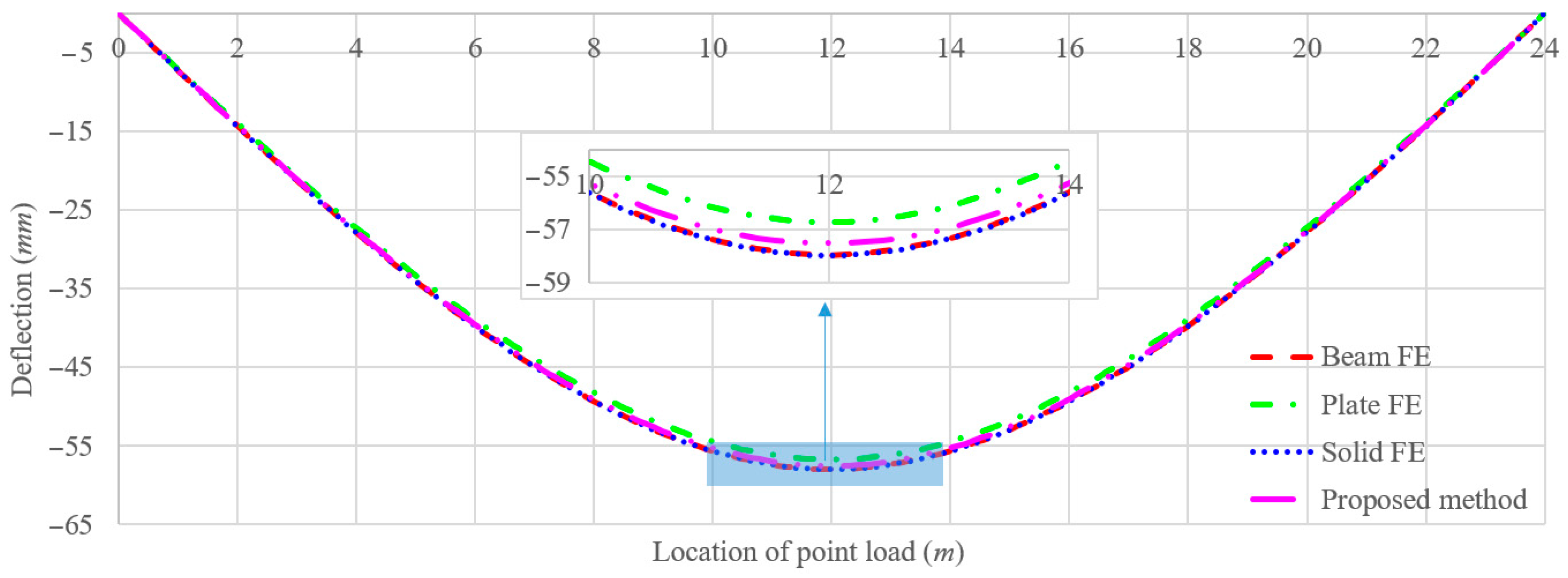
4. Results and Discussion

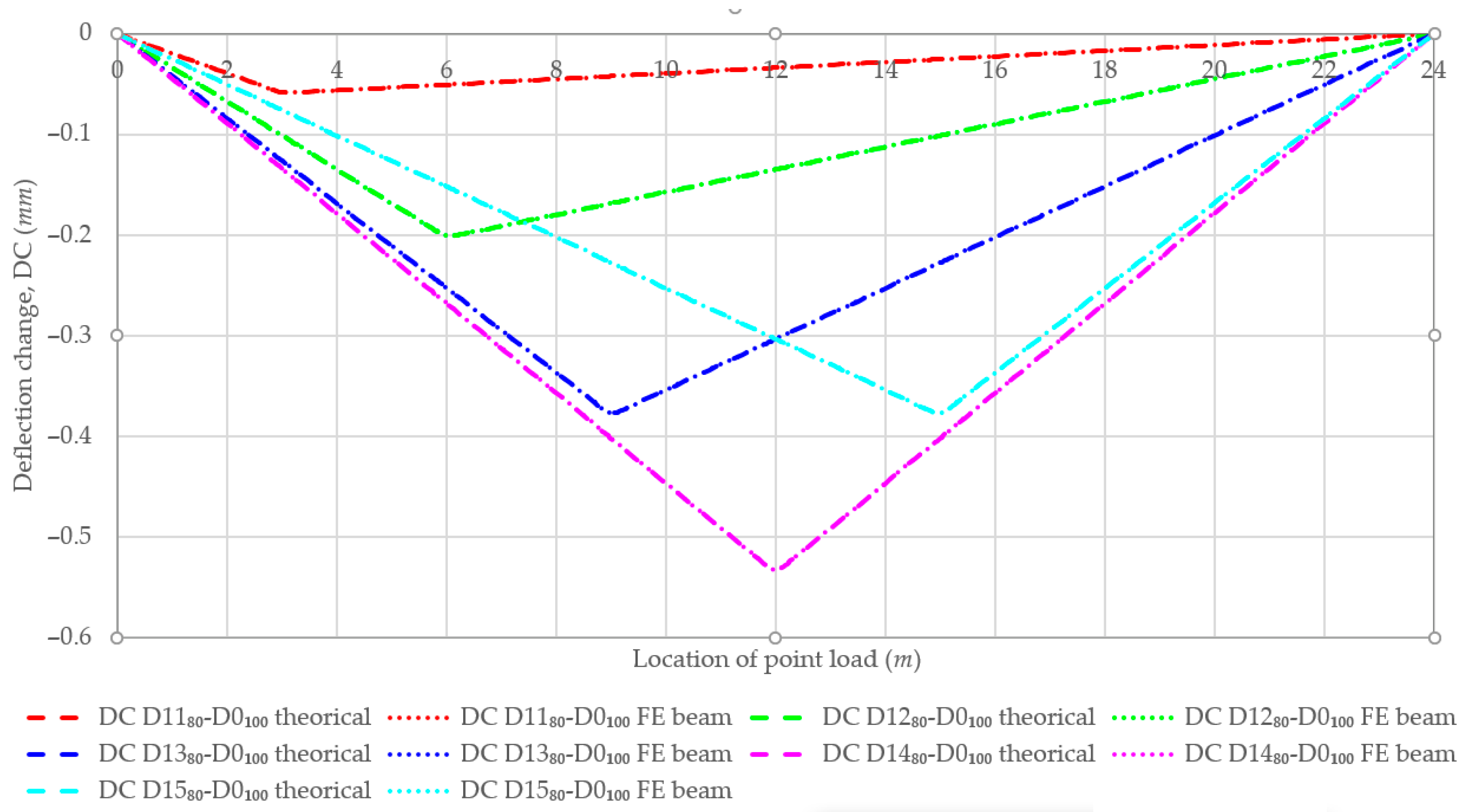
4.1. Single-Damage Beams with Different Positions and Same Remaining Stiffness

The DCs at mid-span points between beams with single damage zones and intact beams in five cases of 1-1 to 1-5 are depicted in Figure 13. Furthermore, Figure 14 and Figure 15 illustrate the first and second derivatives of these DCs, respectively. It is evident from these figures that the results obtained from the proposed method align perfectly with those obtained via the numerical method when using Midas FEA across all case studies, underscoring the accuracy of the theoretical equations developed in this study.

Moreover, considering the same damage index, the change in mid-span deflection increases as the damage zone approaches the mid-span point, as shown in Figure 13. Notably, the case of damage occurring at the mid-span point (case 1-4) yields the maximum DC value (−0.5325 mm), whereas the damage case at L/8 of the beam (case 1-1) results in the smallest DC value (−0.0587 mm), as depicted in Figure 13. This implies that the values of the first and second derivatives of the DC are greatest when the damage zone is at the mid-span point, as illustrated in Figure 14 and Figure 15.

Furthermore, Figure 14 demonstrates that the first derivative of DC remains constant on the left and right sides of the damage position, albeit with differing values. For instance, in case 1-4 with the damage zone at the mid-span point, the first derivative of DC is −4.466 × 10⁻⁵ on the left side and 4.466 × 10⁻⁵ on the right side. Conversely, within the damaged beam section, the value of the first derivative of DC varies. This observation is more apparent in Figure 15, where the second derivative of DC is zero on the left and right sides but non-zero within the damaged beam section.

As described in Section 2.2, the DC, along with its first or second derivatives, as well as the deflection of the intact beam, can be utilized to calculate the damage index and the remaining stiffness. For example, in cases 1-3, where the deflection at the location of 8850 mm equals −52.468 mm and the DC is −0.3728 mm, these values aid in determining the damage index (0.25) and the remaining stiffness (80%), given that the parameters a and b are equal to 8850 mm and 300 mm, respectively, as mentioned in Section 2.5.

4.2. Single-Damage Beam with the Same Positions and Different Remaining Stiffness

Figure 16 shows the deflection changes between beams with single damage zones and intact beam across four cases, denoted as 2-1 to 2-4. The first and second derivatives of these DCs are illustrated in Figure 17 and Figure 18, respectively. Case 2-1, characterized by the smallest remaining stiffness of 60%, exhibits the highest DC value, recorded at −1.005 mm, as evident in Figure 16. Conversely, as the remaining stiffness of the damage zone increases, the deflection change diminishes, reaching −0.1675 mm in cases 2-4. Notably, dividing each DC function (of the above four cases) by the expression (1 − f)/f (of each case) yields a unique function independent of f, but it is solely dependent on the parameters a, b, and l, as mentioned in Section 2.1. Furthermore, it is noteworthy that in these four cases, the intersection zone between the two first-order lines of the DC function in Figure 16 remains consistent. This zone corresponds to the section where the value of the first derivative of DC varies, as illustrated in Figure 17, and the region where the second derivative of DC values is non-zero, as shown in Figure 18. The results obtained for DC, and the 1st and 2nd derivatives of DC from both the proposed model and the numerical model, are very close to each other. Therefore, the following sections will only refer to the proposed model.

4.3. Beam with Multiple Damage Zones Compared to Intact Beam

Figure 19, Figure 20 and Figure 21 present the deflection changes and their first and second derivatives in scenarios involving beams with two or four damage zones compared to intact beams, respectively. Similar to the preceding scenarios, the damage zone is identified at the intersection between the first-order lines of DC, as shown in Figure 19. This intersection also corresponds to the zone of value change for the first derivative of DC in Figure 20, or the section with non-zero values of the second derivative of DC in Figure 21. Furthermore, the number of damage zones equals the number of first-order lines of DC in Figure 19, minus one. It also corresponds to the number of value change segments of the first derivative of DC in Figure 20 or the number of non-zero zones of the second derivative of DC in Figure 21.

As described in Section 2.2, the remaining stiffness or damage index can be calculated by using the ratio of the DC, the first or second derivatives of DC, and the deflection of the intact beam. This calculation is performed using Equations (15)–(17). The remaining stiffness values are illustrated in Figure 21. Additionally, the figures demonstrate that in case 3-1 (D31¹_90%.D31²_90%), where the two damages are symmetric across the mid-span point, the diagram of DC, and its first and or second derivatives are all symmetric. The DC value at the location of the damage zones is equal to −0.2696 mm. In case 3-3, with the same remaining stiffness (scenario D33¹_80%.D33²_80%), the maximum DC value is found at the damage location closest to the mid-span point.

When the two new damage zones appear, as considered in cases 3-1 (D31¹_90%.D31²_90%), 3-2 (D32¹_80%.D32²_90%), 3-3 (D33¹_80%.D33²_80%), and 3-4 (D34¹_70%.D34²_75%), the maximum DC values gradually increase, rising in an inversely proportional manner to the remaining stiffness. These four cases reach the greatest values of −0.2696 mm, −0.5571 mm, −0.8370 mm, and −1.2324 mm, respectively, as illustrated in Figure 19. Additionally, in case 3-5 (D35¹_75%.D35²_70%.D35³_70%.D35⁴_75%), with four damage zones, the second derivative of DC exhibits four non-zero values zones corresponding to four damage zones, as presented in Figure 21.

4.4. Beam with Multiple Damage Zones Considering New Damages and Development of Existing Damages

Figure 22, Figure 23 and Figure 24 illustrate the deflection changes and their first and second derivatives, considering new damages and the development of existing damage, respectively. In Figure 22, the DC in case 4-1 (D41_80% → D41_60%) demonstrates the ongoing deterioration process of this beam, as the remaining stiffness decreases from 80% to 60%, represented by a “new” failure at the original damage location. The value of f = 70.6% in Figure 24 is the solution of the equation: (1 − 80%)/80% + (1 − f)/f = (1 − 60%)/60%. In case 4-2, initially, there were two failures at 3/8 and 4/8 length of the beam, with remaining stiffness equal to 80% and 90%, respectively. Later, the remaining stiffness of the first failure was reduced from 80% to 70%, and fell from 90% to 75% for the second one, represented by two “new” failures on the second derivative of DC, as illustrated in Figure 24. The values of f₁ = 84.8% and f₂ = 81.8% in Figure 24 are the solution of the following equations: (1 − 80%)/80% + (1 − f₁)/f₁ = (1 − 70%)/70% and (1 − 90%)/90% + (1 − f₂)/f₂ = (1 − 75%)/75%. In case 4-3 (D43¹_80%.D43²_100% → D43¹_80%.D43²_90%), the number of first-order lines of DC in Figure 22, the number of value change segments of the first derivative of DC in Figure 23, and the number of non-zero zones of the second derivative of DC in Figure 24 indicate that new damage occurs between the first and second structural states, although the beam had two damage zones at the second structural state. This occurs because a damage zone is not developed further. Contrarily, in cases 4-4, one new damage occurs while the existing damage continues developing. Therefore, based on the DC and the first or the second derivative, as illustrated from Figure 22 to Figure 24, there are two new damage zones between the two structural states. In the last case, 4-5, one existing damage zone is not developed further, while the other existing damage zone continues developing and two new damage zones occur. Thus, between two structural states, it can be considered that the beam experiences three new damage zones (represented by the number of first-order lines of DC in Figure 22, which equals four, and the number of value change segments of the first derivative of DC in Figure 23 and the number of non-zero zones of the second derivative of DC in Figure 24, all equal three).

5. Conclusions

This paper introduces a novel method for detecting damages in a simply supported beam. The approach hinges on assessing the changes in deflection values at the mid-span point between two structural states. These alterations, along with the first- or the derivatives of DC, aid in pinpointing damages and determining the damage index. The validation of the proposed theoretical method is achieved through numerical modeling using three numerical models with beam elements, plate elements, and solid elements. Various case studies are conducted, encompassing scenarios like (1) single-damage beams with different positions but identical remaining stiffness, (2) single-damage beams with consistent positions but varying remaining stiffness, (3) multiple damage zones in comparison to an intact beam, and (4) multiple damage zones with consideration of new damage zones and the progression of existing damage. The results from these case studies confirm the effectiveness of the method in accurately identifying damage locations and calculating damage indices. Furthermore, this method can be extended to locate damage and calculate damage indices using the deflection of any point, not just the mid-span location. However, the comments provided in this study are solely reliant on the proposed method and numerical simulations, excluding experimental data. In practical scenarios, noises may occur and potentially influence measurement outcomes, consequently impacting the identification of the damage location and damage index. Further research should incorporate beam networks (that include both longitudinal and cross beams), examine essential experiments, and analyze the impact of random measurement noise.

References

1. Chan, T.; Thambiratnam, D.P. (Eds.) Structural Health Monitoring in Australia; UK ed. Edition; Nova Science: New York, NY, USA, 2011; pp. 1–193. [Google Scholar]
2. Farrar, C.; Worden, K. Structural Health Monitoring A Machine Learning Perspective, 1st ed.; Wiley: West Sussex, UK, 2012; pp. 1–656. [Google Scholar]
3. Balageas, D.; Fritzen, C.P.; Güemes, A. Structural Health Monitoring; John Wiley & Sons: Hoboken, NJ, USA, 2010; pp. 1–496. [Google Scholar]
4. Yan, R.; Chen, X.; Mukhopadhyay, S.C. Structural Health Monitoring: An Advanced Signal Processing Perspective; Springer International Publishing: Berlin/Heidelberg, Germany, 2017; pp. 1–375. [Google Scholar]
5. Zhang, W.; Li, J.; Hao, H.; Ma, H. Damage detection in bridge structures under moving loads with phase trajectory change of multi-type vibration measurements. Mech. Syst. Signal Process. 2017, 87, 410–425. [Google Scholar] [CrossRef]
6. Wickramasinghe, W.R.; Thambiratnam, D.P.; Chan, T.H.T.; Nguyen, T. Vibration characteristics and damage detection in a suspension bridge. J. Sound Vib. 2016, 375, 254–274. [Google Scholar] [CrossRef]
7. Baba, S.; Kondoh, J. Damage evaluation of fixed beams at both ends for bridge health monitoring using a combination of a vibration sensor and a surface acoustic wave device. Eng. Struct. 2022, 262, 114323. [Google Scholar] [CrossRef]
8. Seyedpoor, S.M.; Yazdanpanah, O. An efficient indicator for structural damage localization using the change of strain energy based on static noisy data. Appl. Math. Model. 2014, 38, 2661–2672. [Google Scholar] [CrossRef]
9. Nguyen, D.H.; Nguyen, Q.B.; Bui-Tien, T.; De Roeck, G.; Wahab, M.A. Damage detection in girder bridges using modal curvatures gapped smoothing method and Convolutional Neural Network: Application to Bo Nghi bridge. Theor. Appl. Fract. Mech. 2020, 109, 102728. [Google Scholar] [CrossRef]
10. Wan, H.; Gao, L.; Yuan, Z.; Qu, H.; Sun, Q.; Cheng, H.; Wang, R. A novel transformer model for surface damage detection and cognition of concrete bridges. Expert Syst. Appl. 2023, 213, 119019. [Google Scholar] [CrossRef]
11. Gordan, M.; Razak, H.A.; Ismail, Z.; Ghaedi, K.; Tan, Z.X.; Ghayeb, H.H. A hybrid ANN-based imperial competitive algorithm methodology for structural damage identification of slab-on-girder bridge using data mining. Appl. Soft Comput. 2020, 88, 106013. [Google Scholar] [CrossRef]
12. Chen, L.; Chen, W.; Wang, L.; Zhai, C.; Hu, X.; Sun, L.; Tian, Y.; Huang, X.; Jiang, L. Convolutional neural networks (CNNs)-based multi-category damage detection and recognition of high-speed rail (HSR) reinforced concrete (RC) bridges using test images. Eng. Struct. 2023, 276, 115306. [Google Scholar] [CrossRef]
13. Kamariotis, A.; Chatzi, E.; Straub, D. A framework for quantifying the value of vibration-based structural health monitoring. Mech. Syst. Signal Process. 2023, 184, 109708. [Google Scholar] [CrossRef]
14. Kouhpangi, M.Z.; Yaghoubi, S.; Torabipour, A. Improved Structural Health Monitoring Using Mode Shapes: An Enhanced Framework for Damage Detection in 2D and 3D Structures. Eng 2023, 4, 1742–1760. [Google Scholar] [CrossRef]
15. Doebling, S.; Farrar, C.; Prime, M. A Summary Review of Vibration-Based Damage Identification Methods. Shock. Vib. Dig. 1998, 30, 91–105. [Google Scholar] [CrossRef]
16. Farrar, C.; Czarnecki, J.J.; Sohn, H.; Hemez, F. A Review of Structural Health Monitoring Literature: 1996–2001; Los Alamos National Laboratory: Santa Fe, NM, USA, 2004; pp. 1–301. [Google Scholar]
17. Fan, W.; Qiao, P. Vibration-based Damage Identification Methods: A Review and Comparative Study. Struct. Health Monit. 2010, 10, 83–111. [Google Scholar] [CrossRef]
18. Cuadrado, M.; Pernas-Sánchez, J.; Artero-Guerrero, J.A.; Varas, D. Detection of barely visible multi-impact damage on carbon/epoxy composite plates using frequency response function correlation analysis. Measurement 2022, 196, 111194. [Google Scholar] [CrossRef]
19. Zhang, H.; Wu, Q.; Xu, W.; Xiong, K. Damage evaluation of complex composite structures using acousto-ultrasonic detection combined with phase-shifted fiber Bragg grating and dual-frequency based data processing. Compos. Struct. 2022, 281, 115000. [Google Scholar] [CrossRef]
20. Moughty, J.J.; Casas, J.R. A State of the Art Review of Modal-Based Damage Detection in Bridges: Development, Challenges, and Solutions. Appl. Sci. 2017, 7, 510. [Google Scholar] [CrossRef]
21. Le, N.T.; Thambiratnam, D.P.; Nguyen, A.; Chan, T.H.T. A new method for locating and quantifying damage in beams from static deflection changes. Eng. Struct. 2019, 180, 779–792. [Google Scholar] [CrossRef]
22. Wang, R.; Zhang, T.; Liu, X.; Lu, Z.; Guo, T. Distance-restrained atmospheric parameters correction (DR-APC) model for GB-SAR transmission power attenuation compensation in bridges dynamic deflection measurement. Measurement 2022, 205, 112192. [Google Scholar] [CrossRef]
23. Zhu, J.; Zhang, C.; Lu, Z.; Li, X. A multi-resolution deep feature framework for dynamic displacement measurement of bridges using vision-based tracking system. Measurement 2021, 183, 109847. [Google Scholar] [CrossRef]
24. White, R.E.; Alexander, N.A.; Macdonald, J.H.G.; Bocian, M. Characterisation of crowd lateral dynamic forcing from full-scale measurements on the Clifton Suspension Bridge. Structures 2020, 24, 415–425. [Google Scholar] [CrossRef]
25. Chen, Z.; Xie, Z.; Zhang, J. Measurement of Vehicle-Bridge-Interaction force using dynamic tire pressure monitoring. Mech. Syst. Signal Process. 2018, 104, 370–383. [Google Scholar] [CrossRef]
26. Rana, S.; Adhikary, S.; Tasnim, J. A statistical index based damage identification method of a bridge using dynamic displacement under moving vehicle. Structures 2022, 43, 79–92. [Google Scholar] [CrossRef]
27. Hu, H.; Wang, J.; Dong, C.Z.; Chen, J.; Wang, T. A hybrid method for damage detection and condition assessment of hinge joints in hollow slab bridges using physical models and vision-based measurements. Mech. Syst. Signal Process. 2023, 183, 109631. [Google Scholar] [CrossRef]
28. Ma, L.L.; Wu, H.; Fang, Q. Damage mode and dynamic response of RC girder bridge under explosions. Eng. Struct. 2021, 243, 112676. [Google Scholar] [CrossRef]
29. Alemu, Y.L.; Lahmer, T.; Walther, C. Damage Detection with Data-Driven Machine Learning Models on an Experimental Structure. Eng 2024, 5, 629–656. [Google Scholar] [CrossRef]
30. Pan, B.; Tian, L.; Song, X. Real-time, non-contact and targetless measurement of vertical deflection of bridges using off-axis digital image correlation. NDT E Int. 2016, 79, 73–80. [Google Scholar] [CrossRef]
31. Pan, P.; Xing, C.; Bai, J.; Yu, S.; Xu, Y.; Zhou, J.; Yu, J. A remote deflection detection method for long-span bridges using adaptive mask and high-resolution camera. Measurement 2022, 201, 111774. [Google Scholar] [CrossRef]
32. Sung, S.H.; Koo, K.Y.; Jung, H.Y.; Jung, H.J. Damage-induced deflection approach for damage localization and quantification of shear buildings: Validation on a full-scale shear building. Smart Mater. Struct. 2012, 21, 115013. [Google Scholar] [CrossRef]
33. Ma, Q.; Solís, M.; Galvín, P. Wavelet analysis of static deflections for multiple damage identification in beams. Mech. Syst. Signal Process. 2021, 147, 107103. [Google Scholar] [CrossRef]
34. Cao, M.; Ye, L.; Zhou, L.; Su, Z.; Bai, R. Sensitivity of fundamental mode shape and static deflection for damage identification in cantilever beams. Mech. Syst. Signal Process. 2011, 25, 630–643. [Google Scholar] [CrossRef]
35. Ghali, A.; Neville, A.; Brown, T. Structural Analysis: A Unified Classical and Matrix Approach, 7th ed.; CRC Press: Boca Raton, FL, USA, 2017; pp. 1–962. [Google Scholar]
36. Midas FEA NX 2020 (v1.1), User Manual; MIDAS Information Technology Co., Ltd.: New York, NY, USA, 2020.
Figure 1. Intact simply supported beam: (a) general layout; (b) real bending moment; (c) virtual bending moment.
Eng 05 00048 g001aEng 05 00048 g001b
Figure 2. Simply supported beam with a single-damage zone located on (a) the left-half beam, (b) the mid-span point, and (c) the right-half beam.
Eng 05 00048 g002
Figure 3. Deflection change Δy10 of SS beam with a single damage zone.
Eng 05 00048 g003
Figure 4. The first derivative of deflection change Δy10.
Eng 05 00048 g004
Figure 5. The second derivative of deflection change Δy10.
Eng 05 00048 g005
Figure 6. Simply supported beam with two damages.
Eng 05 00048 g006
Figure 7. Deflection change Δy21 between SS beams with one and two damage zones.
Eng 05 00048 g007
Figure 8. Deflection change Δy20 between intact beam and beam with two damaged locations.
Eng 05 00048 g008
Figure 9. Deflection change ΔyN0 between intact beam to beam with N damage zones.
Eng 05 00048 g009
Figure 10. Cross-section of beam.
Eng 05 00048 g010
Figure 11. Finite element model: (a) beam element, (b) plate element, (c) solid element.
Eng 05 00048 g011
Figure 12. Mid-span deflection of the intact SS beam.
Eng 05 00048 g012
Figure 13. Mid-span deflection changes with one damage point at different positions.
Eng 05 00048 g013
Figure 14. The first derivative of mid-span deflection changes with one damage zone at different positions.
Eng 05 00048 g014
Figure 15. The second derivative of mid-span deflection changes with one damage zone at different positions.
Eng 05 00048 g015
Figure 16. Mid-span deflection changes with one damage zone at the same position and different remaining stiffness.
Eng 05 00048 g016
Figure 17. The first derivative of mid-span deflection changes with one damage zone at the same position and different remaining stiffness.
Eng 05 00048 g017
Figure 18. The second derivative of mid-span deflection changes with one damage zone at the same position and different remaining stiffness.
Eng 05 00048 g018
Figure 19. Mid-span deflection changes with multiple damage zones compared to an intact beam.
Eng 05 00048 g019
Figure 20. The first derivative of mid-span deflection changes with multiple damage zones compared to an intact beam.
Eng 05 00048 g020
Figure 21. The second derivative of mid-span deflection changes with multiple damages compared to the intact zone.
Eng 05 00048 g021
Figure 22. Mid-span deflection changes with multiple damages considering new damages and development of existing damages.
Eng 05 00048 g022
Figure 23. The first derivative of mid-span deflection changes with multiple damages considering new damages and the development of existing damages.
Eng 05 00048 g023
Figure 24. The second derivative of mid-span deflection changes with multiple damages considering new damages and the development of existing damages.
Eng 05 00048 g024