Abstract
Rail traction and resistance play an essential role in the efficient operation of rail systems. The nature of traction is based on the balance between static friction and generated force at the perimeter of the driving wheels. The main objective of this paper is the development of a methodology and a modeling procedure for the design of train speed trajectory diagrams for the suburban railway. The model is applied to the Athens–Chalkida railway line (in Greece). For this purpose, geometric data for the above-mentioned railway line is collected from the Hellenic Railways Organization (OSE) and then recorded and digitized. A code is developed in MATLAB to calculate the total resistance of the railway line at each kilometer position. The traction elements of the trains operating on the Athens–Chalkida–Athens line, as well as other representative trains, and the magnitudes of their mechanical-aerodynamic resistances are recorded. The MATLAB program generates and compiles the train speed trajectory diagrams and the traction-resistance matrices. Finally, a comparison is made between the time, energy, CO2 emissions, and fuel costs of the rail in relation to the competing mode of transportation, which, for the specific line studied, is the tourist bus.
1. Introduction
The problem of train speed trajectory optimization has received considerable attention due to its impact on operational efficiency, passenger comfort and environmental sustainability. A key aspect of this optimization process is the development of methodological approaches for calculating the total resistance of trains and for designing train speed trajectories. According to [1], the first experiments on the aerodynamic resistance of trains were carried out in the USA in 1906. The purpose was to calculate the aerodynamic resistance of tram trains. In 1910, Schmidt and Dunn [2] published a set of empirical equations describing the aerodynamic resistance of commercial trains for speeds at to 40 mph. Similarly, Strahl, Davis [3], and Protopapadakis [4] developed a formula for calculating running resistance. Over the years, there have been several modifications to make these equations more accurate.
At the same time, trajectory diagrams provide a visual representation of train speed over time, providing insight into the analysis and improvement of railway operations. There is a significant research advancement that explores and investigates various advances and methodological modeling approaches for the design of train speed trajectory diagrams in suburban railway systems. In 1992, Radosavljevic [5] proposed a method for determining the basic traction characteristics of railway vehicles from experimental data. Albrecht et al. [6] described the train motion based on the kinematic equations and calibrated the parameters (speed and acceleration). The authors generated speed profiles for a four-track Dutch railway line using an algorithm developed in MATLAB 2018. Razmjou [7] also developed a software tool in the MATLAB programming language that simulated the movement of a train and calculated the power flow according to the movement of several trains and their schedules. Jong and Chang, [8] developed a simulation program in the C++ language using the object-oriented programming concept to generate speed curves with the shortest operation time and speed profiles with the current operation time and possible energy savings. The authors demonstrated their model on the Taichung line in Taiwan.
A number of researchers have used GPS, train event recorders and real-time predictions. Medeossi et al. [9] used a dynamic equation for each phase of the train movement (acceleration, movement, braking) and calibrated the corresponding parameters with GPS data on board the trains. The method introduced stochastic elements into the motion sequence. The modeling approach was applied to the Trieste–Venice double line. Kecman and Goverde [10] proposed a method for real-time data that represented the path diagrams by graphs that evolve dynamically each time new information is collected. The method was tested for one day on the Dutch railways (in the areas of The Hague and Rotterdam).
Optimization techniques have also been used as modeling approaches to design optimal train speed trajectory diagrams but also to utilize energy data to optimize the operation of a railway line [11,12,13,14,15]. Wang et al. [16] proposed a method for constructing path diagrams using mixed problem integer linear programming (MILP) and a pseudospectral method, while some years later Wang and Goverde [17] formulated a multiple-phase train trajectory optimal control model. Bešinovic et al. [18] used an optimization-based simulation method to calibrate the train force parameters by using input data from the Dutch railway undertaking, where the Rotterdam–Delft corridor was used as a case study. Havaei and Sandidzadeh [19] applied a heuristic algorithm (conscious search) to determine the optimal speed profile. Zeng et al. [20] combine Newtonian physics and expert experience, as well as the use of big data, and propose a method to automatically generate virtual path diagrams.
The above literature highlights significant advancements and diverse methodological approaches regarding the methodology for train speed trajectory diagrams in suburban railway. The researchers used approaches that determined traction characteristics from experimental data, optimization algorithms with real-time data, as well as software tools and programming languages to simulate train movements and generate speed profiles. All methods were validated using real-life case studies, emphasizing their practical applicability. However, their practical implementation is limited by data dependency (availability and accuracy of data from GPD, train recorders, and real-time data sources), computational complexity (due to the application of advanced optimization techniques that can be computationally intensive) and also by differences in infrastructure, operational procedures or other regulatory environments across different regions.
The main objective of this research is to develop a methodology for designing speed curve trajectory diagrams for suburban railways. The methodology is applied to the Athens–Chalkida suburban railway line in Greece. For this purpose, geometric elements of the line were collected and recorded from the Greek Railway Organization (OSE), and traction data for five different train classes was were collected. Based on the selected and processed data, a MATLAB program was developed that includes several components, gradually performs calculations based on the collected data, integrates the results to provide as outputs the calibrated parameters of motion equations, resistance and tractive effort equations and finally constructs the speed trajectory diagrams of the selected trains. The program compared the speed of the simulation process with the real speed. Finally, a comparison was made between the train operating on the railway line and a tourist bus in terms of energy consumption and CO2 emissions. The comparison was based on the occupancy rate of the two different transport modes per passenger kilometer and on specific assumptions.
The contribution of the research lies in (a) presenting a novel methodological approach for designing speed trajectory diagrams for suburban rail lines and discussing the main difficulties in data acquisition; (b) developing a computer program and applying it to a real case study that considers an entire railway route for both directions; (c) validating the results and demonstrating the strengths and usefulness of the proposed methodology; and (d) conducting a comparison of key variables between competing transportation modes.
The rest of the paper hosts Section 2, which describes the theoretical background of the elements that determine the total resistance, the traction force, and the consumption of electrical energy. It also analyses the methodological approach for the modeling process followed and describes the data collection process regarding geometric, infrastructural and kinematic data related to the railway line and rolling stock data. Section 3 presents the results produced by the program for 5 selected rolling stocks for comparison reasons, and Section 4 and Section 5 provide an interpretation and a discussion of the main results extracted by the applied methodology, and finally the main conclusions and further future research proposals.
2. Materials and Methods
2.1. Theoretical Background
2.1.1. Train Resistances
Resistances are divided into two categories: (a) those that depend on the track, called line resistances (WL), and (b) those that depend on the movement of the train, called running resistances (WR).
Line resistances (WL) are subdivided into
- •
- Grade resistances (Wi):where, M is the train mass, g is the gravitational acceleration, and α is the slope angle.Wi = M·g·sin(α)
- •
- Curve resistances (Wc),where k is a variable depending on various factors (curvature, axle, rail-wheel profile gauge, etc.), while R (in m) is the radius of the curve [21,22].Wc = k·(1/R)
For all the above calculations, the use of specific resistances is preferred, which refer to the force per ton of train weight [w = W/(M·g)], measured in 1 N/kN.
The Röckl formula was used to process the data and calculate the curve specific resistances [23,24,25]:
wc = 650/(R – 55) [N/kN], R ≥ 300 m
wc = 500/(R – 30) [N/kN], R < 300 m
Running resistances (WR) due to the movement of the trains refer to mechanical resistances and aerodynamic resistances. Most railway organizations use the general form of the Davis equation, which is as follows:
WR = A + B·V + C·V2
A, B, C: Coefficients that can be functions of train characteristics:
A: Determined by the mechanical resistance of the train and is independent of the speed of the train.
B: Determined by various factors that vary from one organization to another, usually determined by the mass of the train.
C: Defined by the effect of air or aerodynamic resistance at the front and rear of the train.
According to [2,26,27] and for good track quality, the running resistance is as follows:
where
WR = λ·M√(10/m) + 0.01·M·V + (K1·S + K2·p·L)·V2 [daN]
λ: parameter depending on the type of rolling stock, wagons, bogies, mass, etc. (e.g., with usual values for SNCF from 0.9 applicable to modern rolling stock to 1.5 applicable to non-homogeneous freight trains [28])
M: train mass (tons)
m: mass per axle (tons)
K1, K2: aerodynamic coefficients of the train (e.g., the shape of the front and rear of the train, the condition of the surface) with values from 20 × 10−4 (for conventional rolling stock) to 9 × 10⁻⁴ (for TGV rolling stock [28])
S: frontal area of the train (m2)
p: partial perimeter of the rolling stock down to the level of the rails (m) (common values around 10 m)
L: length of train (m)
V: train speed (km/h)
1 daN = 10 N
2.1.2. Tractive Force
As for the train tractive effort Fm, produced by the electric motors, it overcomes the friction forces and any resistances, in other words, it is the result of the friction force (FT) minus the resistances (W). The friction force (FT), generated by the wheel-rail interaction, is expressed by the following formula:
where μ is the coefficient of adhesion, it varies with speed and depends on the condition of the rail running surface (dry, wet). In order to ensure smooth movement of the train without wheel slip on the track, it was necessary to accurately determine the adhesion coefficient μ.
FT = M·g·μ [N]
This approach was carried out by using the empirical relationships of Curtius–Kniffler, which provide significant accuracy for speeds up to 160 km/h.
μ = 0.161 + (7.5)/(V + 44), for dry, sanded rail conditions
μ = 0.130 + (7.5)/(V + 44), for wet, sanded rail conditions
The traction force (Fm) generated by the electric motors at the periphery of the wheels is obtained from Equation (10).
where η is the efficiency factor of the electric power system for rolling stock, P is the power in kW, and V is in m/s.
Fm = η·102·P·g/V [N]
Regarding the energy consumption E, the following formula was used.
where Δx is taken as a fixed step of 0.01 m as discussed in Section 2.2. From the CO2 emissions intensity, the CO2 emissions are estimated and the comparison based on the occupancy rate of the two different transport modes per passenger kilometer is further determined.
E = Fm·Δx·η [N]
2.2. Methodological Approach
The proposed methodology was applied to the Athens–Chalkida line in Greece (Figure 1). This is a suburban railway line with a length of 93.1 km, of which 71.4 km are double track and 21.7 km are single track. During the model development, great care was taken to respect and follow the constraints of the New General Subsidy Regulation (NGSR) [29] for the Greek substructure and the referenced literature.
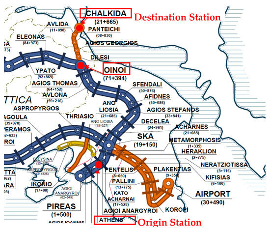
Figure 1.
The Athens–Chalkida suburban railway line in Greece [30].
The methodology followed several different components and sequential steps:
- Collection and manipulation of geometric and infrastructure data from horizontal alignment and longitudinal section maps of the Athens–Chalkida line. A necessary step was to convert these data into a suitable format for further processing in the program. On the basis of this digitized data, a code was created in the MATLAB programming language for the initial processing and calculation of the motion resistances.
- Calculation of total line resistance (WL) per 0.01 m of line length as an output of the program. The choice of 0.01 m length was made because, in this spatial interval, the change in kinematic state is practically negligible, and it allows for a more accurate execution of the program since it segmented the line into 8.1 million positions. With the length of 0.01 m, a constant speed (initial V) was practically considered, which led to more accurate calculation of power and energy. The total line resistance (WL) was calculated as the sum of the resistance due to gradient (Wi) and the resistance due to curvature (Wc).
- Collection and manipulation of kinematic data for the Athens–Chalkida railway line. The knowledge of the speed limits allowed for the calculation of speed profiles per fixed step of 0.01 m.
- Collection of rolling stock data for four different classes of trains and for the train currently operating on the Athens–Chalkida railway line. This step included the digitization of tractive force-speed curve diagrams.
- Design of traction and train speed trajectory diagrams by developing a MATLAB program as an output of the program. The diagrams are made for each of the five different train classes and for both directions, the Athens–Chalkida and the Chalkida–Athens direction routes.
- Calculation of energy consumption and CO2 emissions for the following cases:
- •
- Without electric regenerative braking, where all braking is performed by the friction brakes.
- •
- With regenerative braking, where the braking is assisted by electric motors. In this case, it has been taken into account that all the electricity produced is fed back into the grid, thus reducing the algebraic sum of the energy consumed.
- Comparison of the above results between two different modes of transportation on the Athens–Chalkida route, i.e., train and tourist bus.
2.3. Data Collection
The data collection process was divided into two distinct parts:
- Geometric, infrastructural and kinematic data related to the railway line provided by the Hellenic Railway Organization (OSE). Specifically, the following data were extracted from the horizontal alignment and longitudinal profile maps:
- •
- Length of track sections;
- •
- Gradients per kilometer position;
- •
- Horizontal arcs;
- •
- Kilometer position of the stations along the line;
- •
- Speed limits.
- Rolling stock data. Due to the split of the railway organization responsible for keeping the necessary data, traction data and other train characteristics could not be found. Based on this fact, it was decided that four different classes of trains would be selected as well as the train that is currently operating on the specific rail line in order to perform route simulations. These trains are Z6100 SNCF, BR-423 DB, British Rail Class 450, British Rail Class 800, and Siemens Desiro OSE Series 460 (Table 1). Specifically, the rolling stock data for the above trains (collected from open and public sources as well as train manufacturers) are the following:
 Table 1. Technical characteristics of the selected rolling stock.
- •
- Traction resistance diagrams;
- •
- Number and type of train axles;
- •
- Electrical power characteristics;
- •
- Mass of the trains;
- •
- Train length;
- •
- Maximum speed;
- •
- Number of wagons;
- •
- Year of operation and;
- •
- Seating capacity.
The following assumptions were made for the route simulations: dry rail condition, electrical system efficiency factor for vehicles in service before 2000, η = 0.85, and for vehicles in service after 2000, η = 0.9. These include the losses in the traction circuit, as well as the consumption of auxiliary systems, such as 110 V battery auxiliary consumption and HVAC (Heating Ventilating and Air Conditioning).
3. Results
3.1. Total Line Resistance
To calculate the total line resistance, the model first calculated a number of separate registers: grade resistance, curve resistance, speed, specific grade and specific curve resistance.
Grade resistance registers
The grade data were extracted from the longitudinal section maps of the Athens–Chalkida railway line. The data included a detailed list of the sections with a constant gradient, their beginning, middle and end of the vertical curves, as well as the characteristic elements. During its execution, the algorithm separated the constant gradient sections from the transition areas at the points where the gradients changed. For the constant sections, it recorded the events from the initial kilometer position of the constant gradient section to its final kilometer position, with a fixed step of 0.01 m. These data were stored in the computer’s memory for further processing, and graphs were generated to visualize it.
Curve resistance registers
The model separated the straight lines, where R = ∞→1/R = 0, from the curved lines, where R and 1/R are constant. According to the literature and the Greek NGSR [24], between a straight line and a curve, the curvature 1/R must change linearly from its initial zero value to its final value. The generated curve registers were stored in the computer memory for further processing (Figure 2).

Figure 2.
Curve resistances for the Athens–Chalkida–Athens route.
Figure 2.
Curve resistances for the Athens–Chalkida–Athens route.

Speed registers
The speed values refer to the maximum speed allowed. Unexpected delays in the train operations that occurred during the study period were not taken into account, as they do not represent the typical characteristics of the line. The algorithm manipulated the data to describe the movement of an ideal train that could accelerate at 0.7 m/s2 (the departing train must quickly free the line between the stations of Athens and Oinoi for the national railway network) and decelerate at 0.5 m/s2 (a smooth value tolerable for the passengers).
Specific grade and curve resistance registers
These were derived by applying mathematical equations from Section 2.1. The resulting value is common to all trains, as the final resistance or assistance force when the train is descending is obtained by multiplying this percentage by the weight of the train. By applying the Röckl Equations (3) and (4), the specific curve resistances were calculated.
Total Line Resistance
Now all resistance matrices have the same dimensions as well as the same resistance units (‰), so the final resistance matrix per direction and per station was constructed (Figure 3).

Figure 3.
Total line resistances (a) for the Athens–Chalkida direction and (b) for the Chalkida–Athens direction.
Figure 3.
Total line resistances (a) for the Athens–Chalkida direction and (b) for the Chalkida–Athens direction.

3.2. Results for the Rolling Stock
The simulation ran according to Equations (5) and (6), with modifications to convert units from daN and km/h to N and m/s. Table 2 shows the values for the parameters λ, K1, and K2.
Table 2.
Input values for the parameters λ, K1, K2 for the selected rolling stock.
From the selection and digitalization of geometric, rolling stock and kinematic data, the program generated traction diagrams for all selected rolling stock. Figure 4 presents the diagram of the tractive effort and the running resistance for the Desiro train currently operating in the urban railway line under investigation.
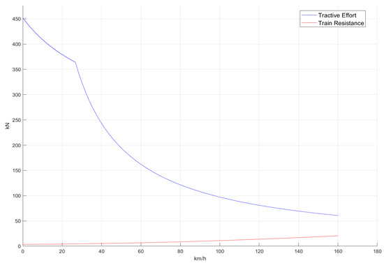
Figure 4.
Traction diagram for the Desiro train.
3.2.1. Speed Trajectories Diagrams
For each train selected, speed trajectory diagrams were generated. The program also compared the simulated speed and the real speed and calculated the total line resistance for each direction, the Athens–Chalkida route (Figure 5) and the return route (Figure 6). It can be seen that the simulated speed–distance trajectory practically overlaps the real speed. Exceptions exist mainly for the Z6100 trains and for the Rail Class 450 and 800 from 20 km to 30 km.
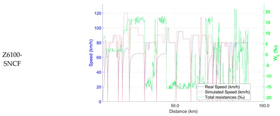
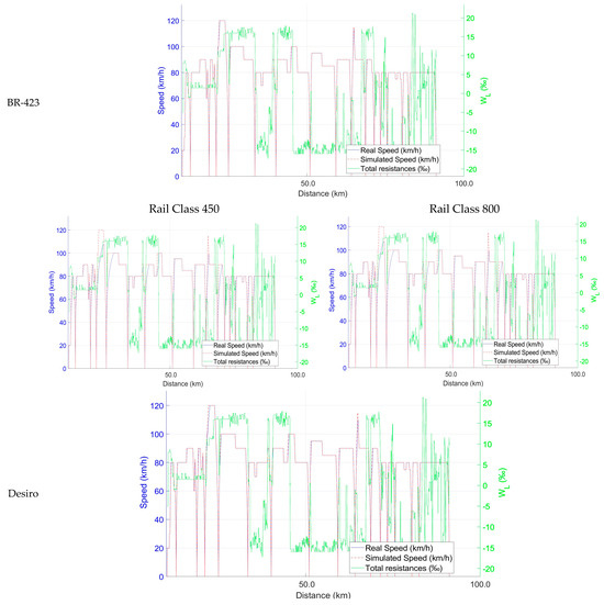
Figure 5.
Comparison of the real speed (magenta line), the simulated speed (dashed line), and the total line resistance for the railway line (green line) for the Athens–Chalkida route.
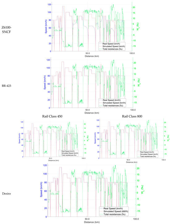
Figure 6.
Comparison of the real speed (magenta line), the simulated speed (dashed line), and the total line resistance for the railway line (green line) for the Chalkida–Athens route.
Furthermore, the program calculated the speed–distance trajectory diagrams and the time–distance diagrams for all rolling stock. Figure 7 shows the output of the trajectory diagrams for the Desiro train currently operating on the rail line.
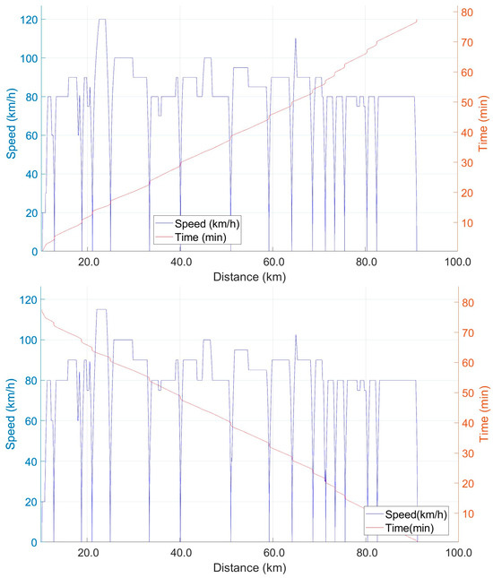
Figure 7.
Speed curve and time–distance trajectories for the Athens–Chalkida route (upper figure) and the Chalkida–Athens route (lower figure) of the Desiro train.
3.2.2. Energy Consumption
The program also estimated the energy consumption for both directions, Athens–Chalkida and Chalkida–Athens for each selected train. The results are further classified into two categories: “without electrical regenerative braking (No RB)” and “with regenerative braking (RB)” (Table 3).
Table 3.
Comparison of energy consumption between the selected rolling stock.
3.2.3. Comparison of Energy Consumption between Train and Bus
The following tables show a comparison of the environmental and energy footprint per passenger kilometer according to the occupancy rate of the two different transport modes. The comparison was made between each selected train and a bus operating on the Athens–Chalkida route. For this case, a Mercedes-Benz Travego bus with 55 seats was considered. The following data assumptions were made:
For the trains:
- •
- Average emissions for each kWh of electricity from the Greek electricity grid of 285 g CO2/kWh (value for 2023, https://www.nowtricity.com/country/greece/, accessed on 20 July 2024).
- •
- Secondary emissions beyond the propulsion of the train are not considered.
- •
- The cost of 1 MWh is €300 (at the time of the analysis, beginning of 2023, from https://www.rae.gr/genika-nea/56333/, accessed on 20 July 2024).
For the bus:
- •
- The average fuel consumption of a 55-seat tourist bus is 25 L/100 km (obtained for the Mercedes-Benz Travego bus from online marketplace for commercial vehicles, e.g., autoline24.gr).
- •
- The thermal power of the diesel engine is 10.96 kWh/L.
- •
- Diesel combustion emissions are 2640 g/kWh.
- •
- The length of the road route is 71.4 km.
- •
- The cost of 1 L of diesel is €1.6.
The Wh/passenger-kilometer was calculated for each train, without electric regenerative braking and with electric braking, assuming an occupancy rate of 10%. Similarly, for the bus. Table 4 shows the results of the above calculations.
Table 4.
Comparison of energy consumption between trains [Table A] and bus [Table B].
It is clear from these tables that the train is the most environmentally friendly inland transportation mode. For example, the Siemens Desiro train with an occupancy rate of 10% without regenerative braking, equivalent to 31 passengers, has a comparable energy consumption of 162 Wh/passKm with the energy consumption of the tourist bus with a 30% occupancy rate, equivalent to 15 passengers (166 Wh/passengerKm).
3.2.4. Comparison of CO2 Emissions between Train and Tourist Bus
A similar procedure was followed to calculate and compare the results of CO2 emissions. The results are shown in Table 5. In this case, the results are even more revealing. In the worst-case scenario for the Siemens Desiro train with a 10% occupancy rate, emissions are 186% lower compared to a fully loaded tourist bus.
Table 5.
Comparison of CO2 between trains [Table A] and bus [Table B].
4. Discussion
During the collection and manipulation of the geometric and infrastructural data of the railway line, it became clear that the line from Athens to Oinoi Station (Figure 1) is based on the major reconstruction carried out in 1964, which improved the railway line that was built years before. However, currently, trains operate at an average speed of 88 km/h due to the small radius curves in the topography. Another limiting factor is the layout of the stations. Except for three stations (the Athens Station, Agioi Anargyroi and Oinoi), all other stations have one track per direction. This significantly limits the overall capacity of the line, as lower-priority services are forced to make long stops to give way to intercity services. In addition, the operation of commercial freight trains during the day is restricted, which has a direct impact on combined transport in Greece.
The railway line from Oinoi station to the destination station of Chalkida underwent extensive reconstruction in the 2000s. However, due to the difficult terrain and the large number of settlements that the line has to serve, the trains operate at an average speed of 78 km/h. However, there are no capacity constraints on this section of the network, as only one train is running on the line at any given time due to the low density of services.
In addition, the program highlighted the environmental advantage of rail over road transportation. A typical 55-seat tourist bus would consume 196 kWh, or 2.74 kWh/km, to complete the route. Similarly, the Siemens Desiro train consumes 411.47 kWh without regenerative braking and 138.17 kWh with regenerative braking, as shown in Table 3. In practice, the train has an average consumption of 5.08 kWh/km without regenerative braking and 1.7 kWh/km with regenerative braking, while the bus consumes 2.74 kWh/km. It can be seen that energy consumption reduction can be achieved from 14% up to approximately 67% by the use of regenerative braking—these are percentages that can be compared and related to other similar studies [interested reader can see [31,32,33,34]].
Even without regenerative braking, the train carries more than 5.6 times as many passengers as the tourist bus. Thus, the energy consumption per kilometer and per passenger is as shown in Table 6:
Table 6.
Comparison of energy consumption per passenger between the Siemens Desiro train and a tourist bus.
In addition, the analysis provided comprehensive results on the energy consumption per passenger-kilometer for different occupancy scenarios. In particular, it was observed that a tourist bus with 50% occupancy, equivalent to 27 passengers, consumes less energy than the Siemens Desiro train with 10% occupancy, equivalent to 31 passengers, when no regenerative braking is used (Table 4). However, in cases where regenerative braking is possible due to the electrical network, energy consumption is significantly lower. As the occupancy of the train increases, its energy efficiency improves. Thus, even with low occupancy and regenerative braking, rail is significantly more energy efficient than road transport. In terms of CO2 emissions, due to the continuous penetration of renewable energy sources, CO2 emissions are significantly lower than those of the tourist bus. A characteristic of this is the fact that even an almost empty train has a much smaller carbon footprint than a full bus per passenger kilometer (Table 5).
Finally, during the program execution, it was observed that trains with a high ratio of traction axles to total axles and high continuous power achieve significant energy production from braking. This trend is more pronounced in trains designed by German companies, as the adhesion requirements in northern countries are higher due to frequent rain and ice.
5. Conclusions
The main objective of this research was to develop a methodology for digitization, programming and design of route diagrams for suburban railway. The methodology was applied to the Athens–Chalkida railway line in Greece. For this purpose, the geometric elements of the line were collected from the Greek Railway Organization (OSE) in order to calculate the total resistance of the railway line per kilometer. The traction data of the trains operating on the Athens–Chalkida–Athens line and the magnitudes of their mechanical-aerodynamic resistances were recorded. The speed trajectory diagrams were designed through the development of a computer program, and a comparison of the simulated route with the actual route was also carried out.
Based on the above, a second comparison was also performed between the selected trains and a tourist bus for evaluating energy consumption and CO2 emissions. The energy consumption and CO2 emissions comparison between trains and bus highlights the environmental benefits and advantages of rail transport and emphasizes its energy efficiency over road transport. This is also justified by the values of 0.016 kWh/km/pax of the train without regenerating braking or 0.005 kWh/km/pax with regenerating braking in comparison to 0.049 kWh/km/pax for the bus. As a result, the train, as a more efficient mode, can move 5.6 times as many passengers as the tourist bus.
The research methodological approach applied to the Athens–Chalkida suburban railway line in Greece, the developed program as well as the validation of the results comparing simulation speeds with actual speeds provide evidence, techniques and data collection processes useful for other similar studies. The comparison of energy consumption and CO2 emissions between the train and bus highlighted the energy efficiency of trains, even with low occupancy rates. The study identifies the importance of rail transportation over road transportation, emphasizing the environmental and energy benefits of trains, especially with the increasing use of renewable energy sources.
In this context, further research for extending the methodology for the design of train speed trajectory diagrams would be an important achievement. The economic benefit of modifying trains with battery systems to benefit directly from regenerative braking could be studied. The use of batteries would relieve the network’s traction system by absorbing the high starting and braking loads. This would create a smarter electric traction network, able to negotiate changes in power consumption profiles to reduce the cost of electricity supply. In addition, an economic feasibility study and a cost-benefit analysis could provide further insights for both national authorities and network operators.
Author Contributions
Conceptualization, T.P.M. and K.L.; methodology, K.K., T.P.M. and K.L.; software, K.K.; validation, T.P.M. and K.L.; formal analysis, K.K.; investigation, K.K.; resources, K.K.; data curation, K.K., T.P.M. and K.L.; writing—original draft preparation, K.K.; writing—review and editing, T.P.M. and K.L.; supervision, T.P.M. All authors have read and agreed to the published version of the manuscript.
Funding
This research received no external funding.
Institutional Review Board Statement
Not applicable.
Informed Consent Statement
Not applicable.
Data Availability Statement
Data available upon request.
Conflicts of Interest
The authors declare no conflicts of interest.
References
- Federal Railroad Administration. Technical Report 7664, “Resistance of a Freight Train to Forward Motion”; Federal Railroad Administration: Cambridge, MA, USA, 1977.
- Schmidt, C.E.; Dunn, H.H. Passenger Train Resistance, Edition «University of Illinois Urbana»; University of Illinois Urbana: Champaign, IL, USA, 1918. [Google Scholar]
- Davis, W.J., Jr. The Tractive Resistance of Electric Locomotives and Cars. In General Electric Review; General Electric: Boston, MA, USA, 1926; p. 3. [Google Scholar]
- Protopapadakis. Notes on Railway Technique; National Technical University of Athens: Athens, Greece, 1925. [Google Scholar]
- Radosavljevic, A. Determination of traction characteristics of diesel locomotives by least square method applied to experimental data. Trans. Model. Simul. 1999, 22, 67–74. [Google Scholar]
- Albrecht, T.; Goverde, R.M.P.; Weeda, V.A.; van Luipen, J. Reconstruction of train trajectories from track occupation data to determine the effects of a driver information system. In Computers in Railways X, WIT Transactions on the Built Environment; Allan, J., Brebbia, C.A., Rumsey, A.F., Sciutto, G., Sone, S., Eds.; WIT Press: Southampton, UK, 2006; Volume 88, pp. 207–216. [Google Scholar]
- Razmjou, S.A. Comprehensive DC Railway Traction System Simulator Based on MATLAB: Tabriz Line 2 Metro Project Case Study. J. Oper. Autom. Power Eng. 2021, 9, 144–159. [Google Scholar]
- Jong, J.C.; Chang, S. Algorithms for generating train speed profiles. J. East. Asia Soc. Transp. Stud. 2005, 6, 356–371. [Google Scholar]
- Medeossi, G.; Longo, G.; de Fabris, S. A method for using stochastic blocking times to improve timetable planning. J. Rail Transp. Plan. Manag. 2011, 1, 1–13. [Google Scholar] [CrossRef]
- Kecman, P.; Goverde, R.M.P. Process mining approach for recovery of realized train paths and route conflict identification. In Proceedings of the 92nd Annual Meeting of the Transportation Research Board, Washington, DC, USA, 13–17 January 2013. [Google Scholar]
- Byun, Y.S.; Jeong, R.G. Optimization of Driving Speed of Electric Train Using Dynamic Programming Based on Multi-Weighted Cost Function. Appl. Sci. 2022, 12, 12857. [Google Scholar] [CrossRef]
- Byun, Y.S.; Jeong, R.G. Optimization of Speed Profiles and Time Schedule of the Urban Rail Transit for Energy-Efficient Operation. IEEE Access 2023, 11, 146030–146041. [Google Scholar] [CrossRef]
- Cao, Y.; Zhang, Z.; Cheng, F.; Su, S. Trajectory Optimization for High-Speed Trains via a Mixed Integer Linear Programming Approach. IEEE Trans. Intell. Transp. Syst. 2022, 23, 17666–17676. [Google Scholar] [CrossRef]
- He, J.; Li, Y.H.; Long, S.H.; Xu, Y.T.; Chen, J.Q. Energy-efficient tram speed trajectory optimization considering the influence of the traffic light. Front. Energy Res. 2022, 10, 963275. [Google Scholar] [CrossRef]
- Wu, C.; Zhang, W.; Lu, S.; Tan, Z.; Xue, F.; Yang, J. Train Speed Trajectory Optimization with On-Board Energy Storage Device. IEEE Trans. Intell. Transp. Syst. 2019, 20, 4092–4102. [Google Scholar] [CrossRef]
- Wang, Y.B.; De Schutter, B.; van den Boom, T.J.J.; Ning, B. Optimal trajectory planning for trains—A pseudospectral method and a mixed integer linear programming approach. Transp. Res. Part C 2013, 29, 97–114. [Google Scholar] [CrossRef]
- Wang, P.; Goverde, R.M.P. Multiple-phase train trajectory optimization with signalling and operational constraints. Transp. Res. Part C 2016, 69, 255–275. [Google Scholar] [CrossRef]
- Bešinovic, N.; Quaglietta, E.; Goverde, R.M.P. A simulation-based optimization approach for the calibration of dynamic train speed profiles. J. Rail Transp. Plan. Manag. 2013, 3, 126–136. [Google Scholar] [CrossRef][Green Version]
- Havaei, P.; Sandidzadeh, M.A. Multi-objective train speed profile determination for automatic train operation with conscious search: A new optimization algorithm, a comprehensive study. Eng. Appl. Artif. Intell. 2023, 119, 105756. [Google Scholar] [CrossRef]
- Zheng, X.; Chen, D.; Lin, Z.; Zhuang, L.; Zhao, W. Method on generating massive virtual driving curves for high-speed trains of the Cross-Taiwan Strait Railway and its statistical analysis. J. Supercomput. 2024, 80, 4202–4225. [Google Scholar] [CrossRef]
- Profillidis, V.A. Railway Management and Engineering; Ashgate: Aldershot, UK, 2006. [Google Scholar]
- Hay, W.W. Railroad Engineering; John Wiley and Sons: New York, NY, USA, 1982. [Google Scholar]
- Schiemann, W. Schienenverkehrstechnik, Grundlagen der Gleistrassierung; s. 81; Teubner: Berlin, Germany, 2002. [Google Scholar]
- Fiedler, J. BAHNWESEN: Planung, Bau und Betriebvon Eisenbahnen, S-, U-Stadt—Und Strassenbahnen, 5. Neu und Erweiterte Auflage; s. 42; Werner Verlag: Bielefeld, Germany, 2005. [Google Scholar]
- Volker, M. “Bahnbau” 7. Auflage; s. 37; Teubner Verlag: Berlin, Germany, 2007. [Google Scholar]
- Karlaftis, M.G.; Lyberis, K. Operation of Public Transport Networks; Editions Symmetria; Symmetria: Athens, Greece, 2008. (In Greek) [Google Scholar]
- Pyrgidis, C. Rail Transport Systems; Editions Ziti; Ziti: Thessaloniki, Greece, 2009. (In Greek) [Google Scholar]
- Rochard, B.P.; Schmid, F. A review of methods to measure and calculate train resistances. Proc. Inst. Mech. Eng. Part F J. Rail Rapid Transit 2000, 214, 185–199. [Google Scholar] [CrossRef]
- New General Subsidy Regulation (NGSR). Govenrment Gazette, Law No 1156/2000. 2000.
- Greek Railway Organisation (OSE). Available online: https://ose.gr/wp-content/uploads/2021/08/english-RAILWAY-MAP_Site-Version.pdf (accessed on 20 May 2024).
- Hoo, D.S.; Chua, K.H.; Lim, Y.S.; Morris, S.; Wang, L. Comparison of regenerative braking energy recovery of a DC third rail system under various operating conditions. Int. J. Electr. Power Energy Syst. 2024, 155, 109575. [Google Scholar] [CrossRef]
- Scheepmaker, G.M.; Goverde, R.M.P. Energy-efficient train control using nonlinear bounded regenerative braking. Transp. Res. Part C Emerg. Technol. 2020, 121, 102852. [Google Scholar] [CrossRef]
- Allen, L.A.; Chien, S.I. Rail Energy Efficiency Improvement by Combining Coasting and Regenerative Braking. Int. J. Railw. Technol. 2018, 7, 1–22. [Google Scholar] [CrossRef]
- Che, C.; Wang, Y.; Lu, Q.; Peng, J.; Liu, X.; Chen, Y.; He, B. An effective utilization scheme for regenerative braking energy based on power regulation with a genetic algorithm. IET Power Electron. 2022, 15, 1392–1408. [Google Scholar] [CrossRef]


Disclaimer/Publisher’s Note: The statements, opinions and data contained in all publications are solely those of the individual author(s) and contributor(s) and not of MDPI and/or the editor(s). MDPI and/or the editor(s) disclaim responsibility for any injury to people or property resulting from any ideas, methods, instructions or products referred to in the content. |
© 2024 by the authors. Licensee MDPI, Basel, Switzerland. This article is an open access article distributed under the terms and conditions of the Creative Commons Attribution (CC BY) license (https://creativecommons.org/licenses/by/4.0/).