
Analysis of Operational Control Data and Development of a Predictive Model of the Content of the Target Component in Melting Products


Abstract
1. Introduction
2. Data Analysis
- − Calculating the sum of the deviations of the average values by columns in the obtained table from the average values of the original;
- − Creating a correlation matrix to determine the relationship between the quantities in the initial and final tables.
- − They were indirect, meaning they do not have a direct impact on the process under consideration;
- − They were significantly damaged.
3. Methods
- All parameters characterizing the furnace load had a sufficiently high correlation (correlation coefficient around 0.6–0.7). This suggests that the operator tried to maintain the required ratio of “charge load—blowing rate” regulated by the protocol. However, this seems to be insufficient, as it did not affect the copper content in the matte (all correlation coefficients were insignificant).
- The feed temperature of the furnace in the smelting zone, although correlated with the furnace load parameters (temperature increased with an increase in overall blast volume—positive correlation, and feed temperature decreased with an increase in charge rate—negative correlation), was relatively weakly correlated (correlation coefficient around 0.15).
4. Results
- (1)
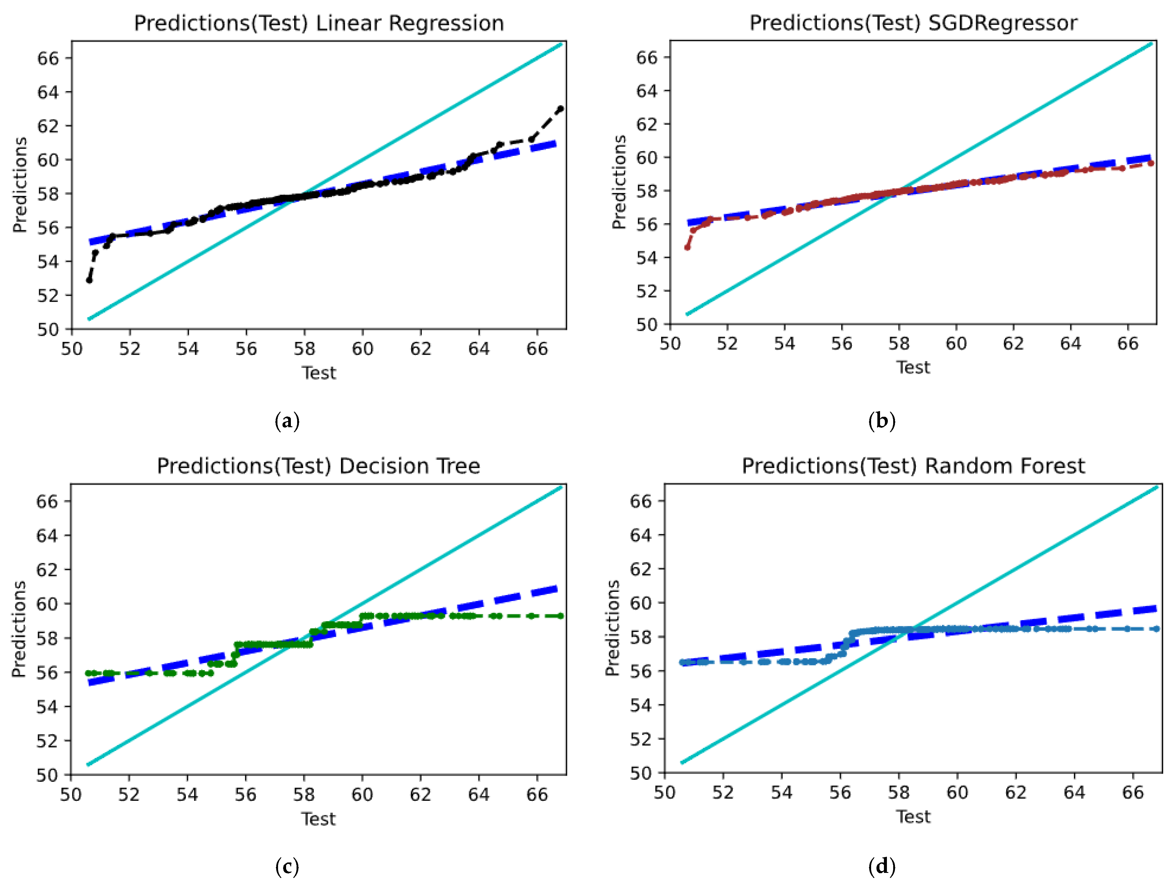
- Linear regression—one of the simplest and widely used methods in machine learning, based on the assumption of a linear relationship between input features and the output variable. Linear regression seeks to find the best straight line that most accurately fits the data.
- (2)
- Stochastic gradient descent (SGDRegressor)—an optimization method for linear regression. Unlike regular linear regression, SGDRegressor updates the model parameters using gradient descent at each iteration.
- (3)
- Decision tree—a machine learning model that makes decisions based on the sequential application of conditions to input data. It builds a tree where each node represents a specific condition, and each leaf node represents a specific prediction.
- (4)
- Random forest—an ensemble machine learning model consisting of multiple decision trees. Each tree is trained on a subset of data and a subset of features. In the end, predictions from each tree are combined to obtain the final prediction.
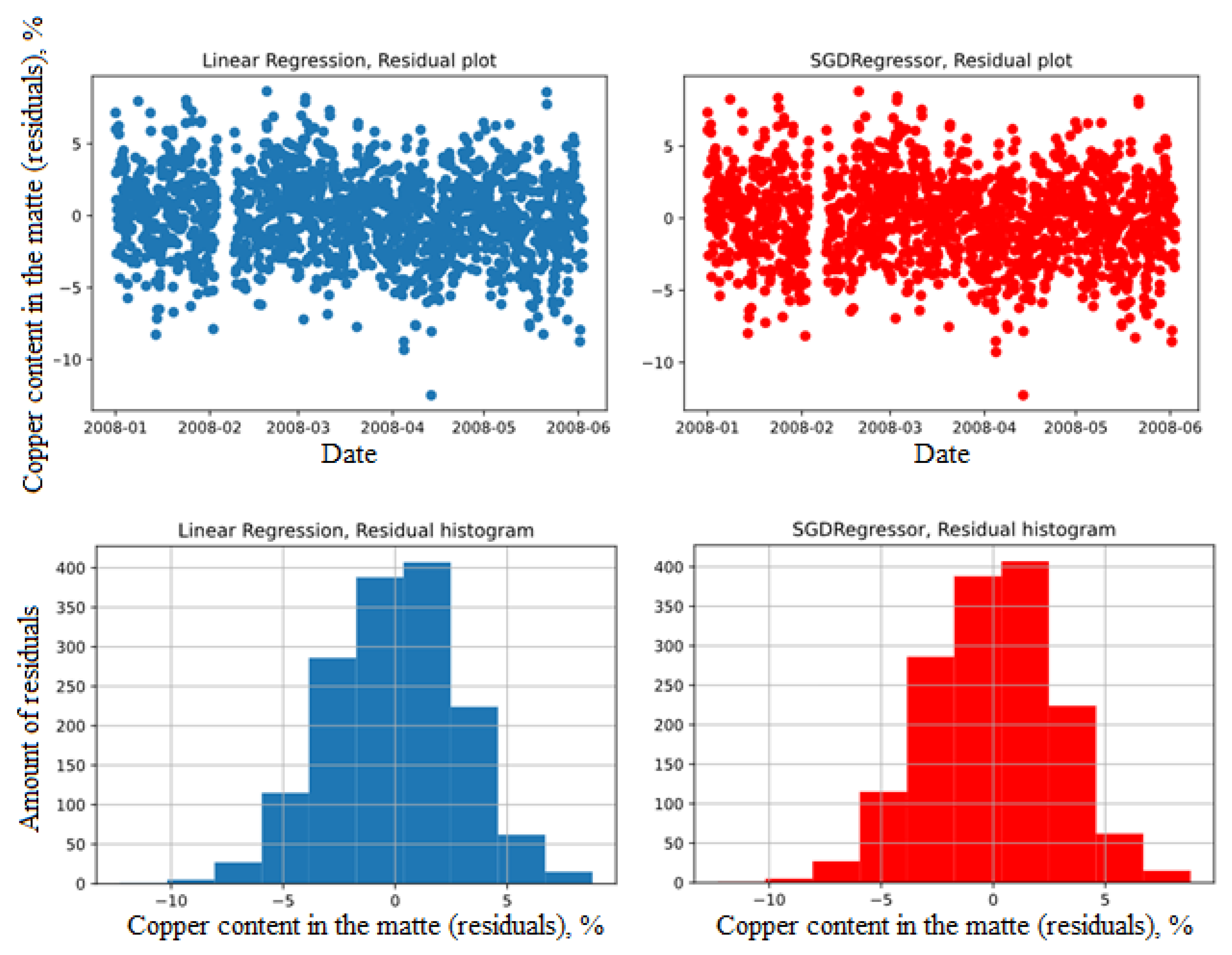
4.1. Linear Regression
- (1)
- Mean absolute error (MAE);
- (2)
- Root mean squared error (RMSE);
- (3)
- Mean absolute percentage error (MAPE);
- (4)
- R-squared score.
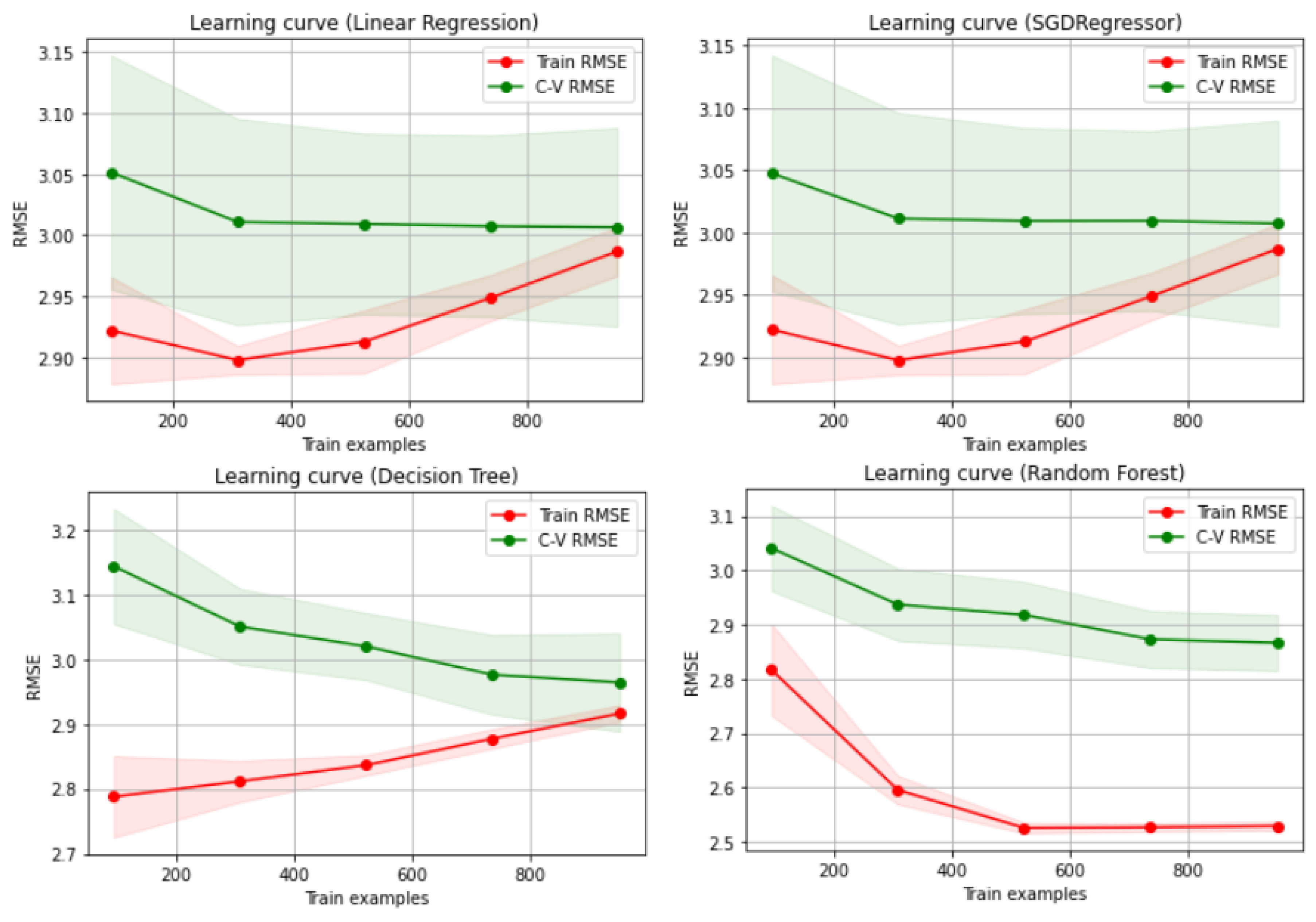
- (1)
- In the graphs of linear models and decision trees, there was no overfitting issue, as the training and test curves were quite close to each other;
- (2)
- Linear regression and stochastic gradient descent models did not improve performance on cross-validation as the training sample increased; therefore, they reached their best RMSE;
- (3)
- The random forest model had better performance on cross-validation, despite its curve showing an overfitting problem.
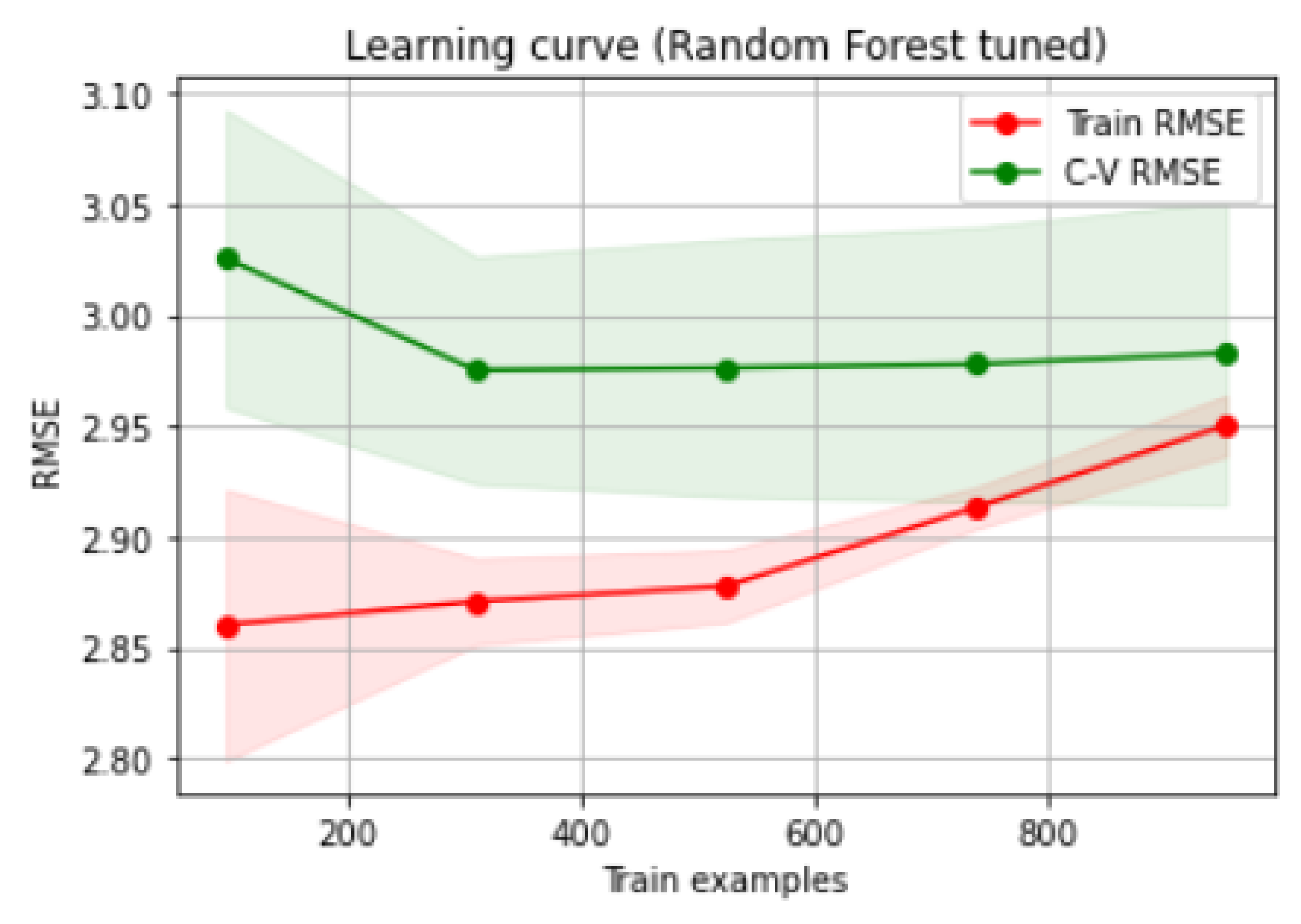
4.2. Addressing the Overfitting Issue
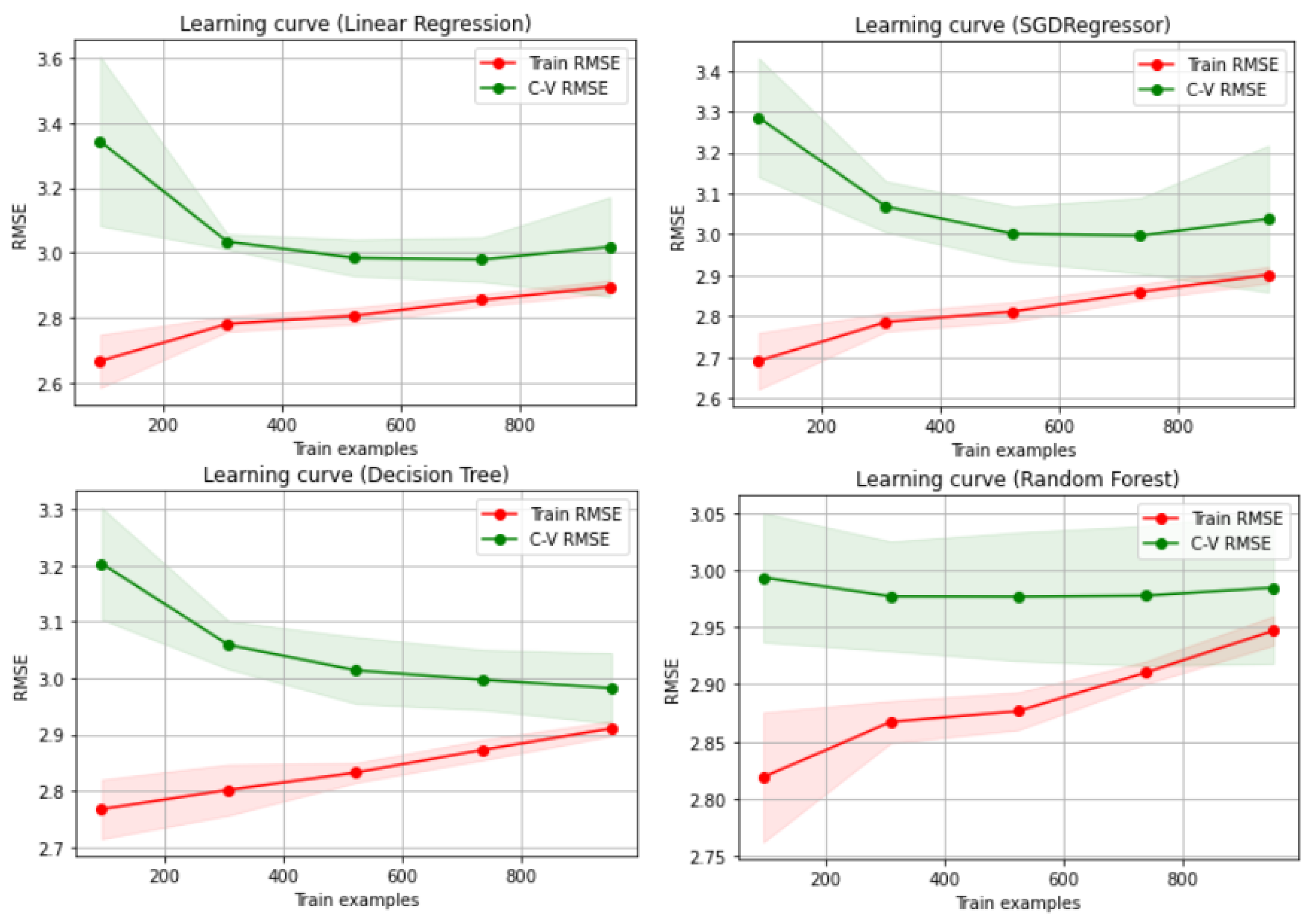
4.3. High Bias Problem and Polynomial Features
5. Conclusions
Author Contributions
Funding
Data Availability Statement
Conflicts of Interest
References
- George, G.; Lavie, D. Big data and data science methods for management research. Acad. Manag. J. 2016, 59, 1493–1507. [Google Scholar] [CrossRef]
- Aazam, M.; Zeadally, S.; Harras, K.A. Deploying fog computing in industrial internet of things and industry 4.0. IEEE Trans. Ind. Inform. 2018, 14, 4674–4682. [Google Scholar] [CrossRef]
- Thillaieswari, B. Comparative Study on Tools and Techniques of Big Data Analysis. Int. J. Adv. Netw. Appl. (IJANA) 2017, 08, 61–66. [Google Scholar]
- Thombansen, U.; Purrio, M.; Buchholz, G.; Hermanns, T.; Molitor, T.; Willms, K.; Schulz, W.; Reisgen, U. Determination of process variables in melt-based manufacturing processes. Int. J. Comput. Integr. Manuf. 2016, 29, 1147–1158. [Google Scholar] [CrossRef]
- Aleksandrova, T.N. Complex and deep processing of mineral raw materials of natural and technogenic origin: State and prospects. J. Min. Inst. 2022, 256, 503–504. [Google Scholar]
- Zhukovskiy, Y.L.; Korolev, N.A.; Malkova, Y.M. Monitoring of grinding condition in drum mills based on resulting shaft torque. J. Min. Inst. 2022, 256, 686–700. [Google Scholar] [CrossRef]
- Oprea, G.; Andrei, H. Power quality analysis of industrial company based on data acquisition system, numerical algorithms and compensation results. In Proceedings of the 2016 International Symposium on Fundamentals of Electrical Engineering, ISFEE, Bucharest, Romania, 30 June–2 July 2016; p. 7803232. [Google Scholar] [CrossRef]
- Wang, H.-Y.; Wu, W.-D. Statistical Process Control Based on Two Kinds of Feedback Adjustment for Autocorrelated Process. In Proceedings of the 2008 4th International Conference on Wireless Communications, Networking and Mobile Computing, Dalian, China, 12–17 October 2008. [Google Scholar] [CrossRef]
- Fahle, S.; Prinz, C.; Kuhlenkötter, B. Systematic review on machine learning (ML) methods for manufacturing processes–identifying artificial intelligence (AI) methods for field application. Procedia CIRP 2020, 93, 413–418. [Google Scholar] [CrossRef]
- Potapov, A.I.; Kulchitskii, A.A.; Smorodinskii, Y.G.; Smirnov, A.G. Evaluating the Error of a System for Monitoring the Geometry of Anode Posts in Electrolytic Cells with Self-Baking Anode. Russ. J. Nondestruct. Test. 2020, 56, 268–274. [Google Scholar] [CrossRef]
- Ilyushin, Y.V.; Kapostey, E.I. Developing a Comprehensive Mathematical Model for Aluminium Production in a Soderberg Electrolyser. Energies 2023, 16, 6313. [Google Scholar] [CrossRef]
- Lutskiy, D.S.; Ignatovich, A.S. Study on hydrometallurgical recovery of copper and rhenium in processing of substandard copper concentrates. J. Min. Inst. 2021, 251, 723–729. [Google Scholar] [CrossRef]
- Nguyen, H.H.; Bazhin, V.Y. Optimization of the Control System for Electrolytic Copper Refining with Digital Twin During Dendritic Precipitation. Metallurgist 2023, 67, 41–50. [Google Scholar] [CrossRef]
- Kolesnikov, A.S. Kinetic investigations into the distillation of nonferrous metals during complex processing of waste of metallurgical industry. Russ. J. Non-Ferr. Met. 2015, 56, 1–5. [Google Scholar] [CrossRef]
- Vasilyeva, N.V.; Fedorova, E.R. Obrabotka bolshogo massiva dannyh operativnogo kontrolya i podgotovka ego k razrabotke avtomatizirovannoj sistemy upravleniya tekhnologicheskim processom. In Promyshlennye ASU i Kontrollery; Scientific & Technical Literature Publishing House: Moscow, Russia, 2019; pp. 3–9, (In Russian). [Google Scholar] [CrossRef]
- Semenova, I.N.; Kirpichenkov, I.A. Development of the control system for temperature conditions of melting process in the Vanyukov furnace. Russ. J. Non-Ferr. Met. 2009, 5, 59–62. [Google Scholar]
- Zhang, H.L.; Zhou, C.Q.; Bing, W.U.; Chen, Y.M. Numerical simulation of multiphase flow in a Vanyukov furnace. J. South. Afr. Inst. Min. Metall. 2015, 115, 457–463. [Google Scholar] [CrossRef]
- Lisienko, V.G.; Malikov, G.K.; Morozov, M.V.; Belyaev, V.V.; Kirsanov, V.A. Modeling heat-and-mass exchange processes in the Vanyukov furnace in specific operational conditions. Russ. J. Non-Ferr. Met. 2012, 53, 272–278. [Google Scholar] [CrossRef]
- Bazhin, V.Y.; Masko, O.N.; Martynov, S.A. Automatic burden balance monitoring and control in the production of metallurgical silicon. Tsvetnye Met. 2023, 4, 53–60. [Google Scholar] [CrossRef]
- Tercan, H.; Meisen, T. Machine learning and deep learning based predictive quality in manufacturing: A systematic review. J. Intell. Manuf. 2022, 33, 1879–1905. [Google Scholar] [CrossRef]
- Dalzochio, J.; Kunst, R.; Pignaton, E.; Binotto, A.; Sanyal, S.; Favilla, J.; Barbosa, J. Machine learning and reasoning for predictive maintenance in industry 4.0: Current status and challenges. Comput. Ind. 2020, 123, 103298. [Google Scholar] [CrossRef]
- Platonov, O.I.; Tsemekhman, L.S. Potential copper plant Vanyukov furnace gas desulphurization capacity. Tsvetnye Met. 2021, 2021, 1–19. [Google Scholar] [CrossRef]
- Ozerov, S.S.; Tsymbulov, L.B.; Eroshevich, S.Y.; Gritskikh, V.B. Looking at the changing composition of blister copper obtained through continuous converting. Tsvetnye Met. 2020, 64–69. [Google Scholar] [CrossRef]
- Fedorova, E.R.; Trifonova, M.E.; Mansurova, O.K. Red mud thickener statistical model in MATLAB system identification toolbox. J. Phys. Conf. Ser. 2019, 1333, 032019. [Google Scholar] [CrossRef]
- Utekhin, G. Use of statistical techniques in quality management systems. In Proceedings of the 8 International Conference Reliability and Statistics in Transportation and Communication–2008, Riga, Latvia, 17–20 October 2018; pp. 329–334. [Google Scholar]
- Shklyarskiy, Y.E.; Skamyin, A.N.; Jiménez Carrizosa, M. Energy Efficiency in the Mineral Resources and Raw Materials Complex. J. Min. Inst. 2023, 261, 323–324. [Google Scholar]
- Yun, J.P.; Shin, W.C.; Koo, G.; Kim, M.S.; Lee, C.; Lee, S.J. Automated defect inspection system for metal surfaces based on deep learning and data augmentation. J. Manuf. Syst. 2020, 55, 317–324. [Google Scholar] [CrossRef]
- Goldman, C.V.; Baltaxe, M.; Chakraborty, D.; Arinez, J. Explaining learning models in manufacturing processes. Procedia Comput. Sci. 2021, 180, 259–268. [Google Scholar] [CrossRef]
- Iwana, B.K.; Uchida, S. An empirical survey of data augmentation for time series classification with neural networks. PLoS ONE 2021, 16, e0254841. [Google Scholar] [CrossRef]
- Schmitt, J.; Boenig, J.; Borggraefe, T.; Beitinger, G.; Deuse, J. Predictive model-based quality inspection using machine learning and edge cloud Computing. Adv. Eng. Inform. 2020, 45, 101101. [Google Scholar] [CrossRef]
- Wu, X.; Zhu, X.; Wu, G.-Q.; Ding, W. Data Mining with Big Data. IEEE Trans. Knowl. Data Eng. 2014, 26, 97–107. [Google Scholar] [CrossRef]
- Rao, J.N.; Ramesh, M. A Review on Data Mining & Big Data, Machine Learning Techniques. Int. J. Recent Technol. Eng. (IJRTE) 2019, 7, 914–916. [Google Scholar]
- Machado, G.; Winroth, M.; Carlsson, D.; Almström, P.; Centerholt, V.; Hallin, M. Industry 4.0 readiness in manufacturing companies: Challenges and enablers towards increased digitalization. CIRP Manuf. Syst. Conf. 2019, 81, 1113–1118. [Google Scholar] [CrossRef]
- Kim, A.; Oh, K.; Jung, J.-Y.; Kim, B. Imbalanced classification of manufacturing quality conditions using cost-sensitive decision tree ensembles. Int. J. Comput. Integr. Manuf. 2018, 31, 701–717. [Google Scholar] [CrossRef]
- Serin, G.; Sener, B.; Gudelek, M.U.; Ozbayoglu, A.M.; Unver, H.O. Deep multi-layer perceptron based prediction of energy efficiency and surface quality for milling in the era of sustainability and big data. Procedia Manuf. 2020, 51, 1166–1177. [Google Scholar] [CrossRef]
- Boikov, A.V.; Payor, V.A. The Present Issues of Control Automation for Levitation Metal Melting. Symmetry 2022, 14, 1968. [Google Scholar] [CrossRef]
- Koteleva, N.I.; Khokhlov, S.V.; Frenkel, I.V. Digitalization in Open-Pit Mining: A New Approach in Monitoring and Control of Rock Fragmentation. Appl. Sci. 2021, 11, 10848. [Google Scholar] [CrossRef]


| Total charge rate, t/h | Overall blast volume, m3/h | Oxygen content in the blast (degree of oxygen enrichment in the blowing), % | Temperature of exhaust gases in the off-gas duct, °C | Temperature of feed in the smelting zone, °C | Copper content in the matte, % | |
|---|---|---|---|---|---|---|
| Total charge rate, t/h | 1.000 | 0.637 | 0.693 | −0.176 | −0.156 | −0.052 |
| Overall blast volume, m3/h | 0.637 | 1.000 | 0.602 | −0.018 | 0.157 | −0.136 |
| Oxygen content in the blast (degree of oxygen enrichment in the blowing), % | 0.693 | 0.602 | 1.000 | 0.006 | −0.005 | −0.155 |
| Temperature of exhaust gases in the off-gas duct, °C | −0.176 | −0.018 | 0.006 | 1.000 | −0.056 | −0.068 |
| Temperature of feed in the smelting zone, °C | −0.156 | 0.157 | −0.005 | −0.056 | 1.000 | −0.146 |
| Copper content in the matte, % | −0.052 | −0.136 | −0.155 | −0.068 | −0.146 | 1.000 |
| Total charge rate, t/h | Overall blast volume, m3/h | Oxygen content in the blast (degree of oxygen enrichment in the blowing), % | Temperature of exhaust gases in the off-gas duct, °C | Temperature of feed in the smelting zone, °C | Copper content in the matte, % | |
|---|---|---|---|---|---|---|
| Total charge rate, t/h | 1.000 | 0.632 | 0.691 | −0.162 | −0.147 | −0.044 |
| Overall blast volume, m3/h | 0.632 | 1.000 | 0.577 | −0.010 | 0.190 | −0.134 |
| Oxygen content in the blast (degree of oxygen enrichment in the blowing), % | 0.691 | 0.577 | 1.000 | 0.0023 | 0.0004 | −0.149 |
| Temperature of exhaust gases in the off-gas duct, °C | −0.162 | −0.010 | 0.023 | 1.000 | −0.033 | −0.069 |
| Temperature of feed in the smelting zone, °C | −0.147 | 0.190 | −0.0004 | −0.033 | 1.000 | −0.170 |
| Copper content in the matte, % | −0.044 | −0.134 | −0.149 | −0.069 | −0.170 | 1.000 |
| Model | MAE | RMSE |
|---|---|---|
| Linear Regression | 2.379 | 3.011 |
| SGDRegressor | 2.374 | 3.007 |
| Decision Tree | 2.385 | 3.009 |
| Random Forest | 2.369 | 3.005 |
| Model | MAE | RMSE |
|---|---|---|
| Linear Regression | 2.169 (−8.8%) | 2.803 (−6.9%) |
| SGDRegressor | 2.153 (−9.3%) | 2.774 (−7.7%) |
| Decision Tree | 2.276 (−4.6%) | 2.930 (−2.6%) |
| Random Forest | 2.254 (−4.9%) | 2.867 (−4.6%) |
Disclaimer/Publisher’s Note: The statements, opinions and data contained in all publications are solely those of the individual author(s) and contributor(s) and not of MDPI and/or the editor(s). MDPI and/or the editor(s) disclaim responsibility for any injury to people or property resulting from any ideas, methods, instructions or products referred to in the content. |
© 2024 by the authors. Licensee MDPI, Basel, Switzerland. This article is an open access article distributed under the terms and conditions of the Creative Commons Attribution (CC BY) license (https://creativecommons.org/licenses/by/4.0/).
Share and Cite
Vasilyeva, N.; Pavlyuk, I. Analysis of Operational Control Data and Development of a Predictive Model of the Content of the Target Component in Melting Products. Eng 2024, 5, 1752-1767. https://doi.org/10.3390/eng5030092
Vasilyeva N, Pavlyuk I. Analysis of Operational Control Data and Development of a Predictive Model of the Content of the Target Component in Melting Products. Eng. 2024; 5(3):1752-1767. https://doi.org/10.3390/eng5030092
Chicago/Turabian StyleVasilyeva, Natalia, and Ivan Pavlyuk. 2024. "Analysis of Operational Control Data and Development of a Predictive Model of the Content of the Target Component in Melting Products" Eng 5, no. 3: 1752-1767. https://doi.org/10.3390/eng5030092
APA StyleVasilyeva, N., & Pavlyuk, I. (2024). Analysis of Operational Control Data and Development of a Predictive Model of the Content of the Target Component in Melting Products. Eng, 5(3), 1752-1767. https://doi.org/10.3390/eng5030092