Modeling and Control of a Permanent Magnet DC Motor: A Case Study for a Bidirectional Conveyor Belt’s Application

Abstract

Direct current (DC) motors are widely used in various applications because of their operational advantages and ease of control compared to those of other rotating machines. This study focuses on regulating the operation of a bidirectional conveyor powered by a permanent magnet DC motor driven by a full H-bridge power converter. The mechatronic system, comprising a conveyor, a DC motor, and a power converter, is modeled using first-order differential equations. For control design purposes, a simplified actuator model is derived, treating the conveyor load as an external disturbance. A linear control scheme, based on classical control theory, is proposed to ensure that the actuator velocity tracks the reference input. To improve the disturbance rejection, particularly against variations in mechanical loads, an extended state observer is incorporated. Simulation tests validated the proposed control scheme, highlighting the functionality and tradeoffs of its internal components.

1. Introduction

Direct current (DC) motors are electrical rotating machines widely used as actuators in various applications [1]. Their popularity is largely because of the advantages they offer, such as a high initial acceleration, torque, and a wide range of angular velocities [2]. Some applications of this rotating machine as an actuator include overhead cranes [3], electric and hybrid vehicles [4], and robotic systems [5], among others. A key factor in regulating the operation of DC motors is that they require minimal adjustments to control their rotor’s angle, angular velocity, or output mechanical torque [2]. These adjustments are typically made using power electronic devices [6].

Several power electronic devices have been proposed to operate as DC motor drive systems [7]. These devices are capable of managing the voltage applied to the electrical input of the motor by adjusting the DC voltage at their output terminal. The changes in the DC level at their output terminal are achieved through modulation techniques, with pulse width modulation being the most commonly used in this application [8].

Ardhenta and Subroto [9] proposed the use of a DC–DC buck converter to regulate the velocity of a permanent magnet DC motor. They employed a linear control scheme tuned using the pole placement technique, along with a state observer to reject external perturbations, such as load torque. A disadvantage of using this power converter as a motor driver is its inability to generate motion in both directions. Liceaga-Castro et al., in [10], employed a full H-bridge to regulate the speed of a series DC motor, enabling bidirectional rotation of the motor’s rotor and allowing the motor to operate in both acceleration and braking modes. In this research, the system model comprising the power converter and the DC motor is derived through identification procedures rather than analytical modeling.

Various control schemes have been proposed to regulate the behavior of DC motors for different applications. These include nonlinear control approaches, such as sliding mode control [11], backstepping-based control [12], passivity-based control [5], and feedback-linearization-based control [13] among others. On the other hand, several conventional linear control schemes have been proposed, such as PI-based controllers [10] and lag or lead compensators [14]. The advantages of implementing such conventional techniques are grounded in two main factors. First, the tuning process for proposing a control scheme allows each component to be thoroughly justified in terms of phase and gain margins. Second, the controller demonstrates robustness and effectiveness despite its simplicity, which typically requires a low level of computational resources. For these reasons, and the antecedent mentioned above, the use of a linear control scheme has been proposed for regulating the operation of the DC motor as an actuator of a bidirectional conveyor.

In the present research, a permanent magnet DC motor controlled by a full H-bridge power converter is considered as an actuator for a conveyor system. The choice of this motor driver is motivated by its ability to enable the bidirectional movement of the conveyor, enhancing its functionality and adaptability for integration into a flexible manufacturing process. The main contributions of this work are as follows:

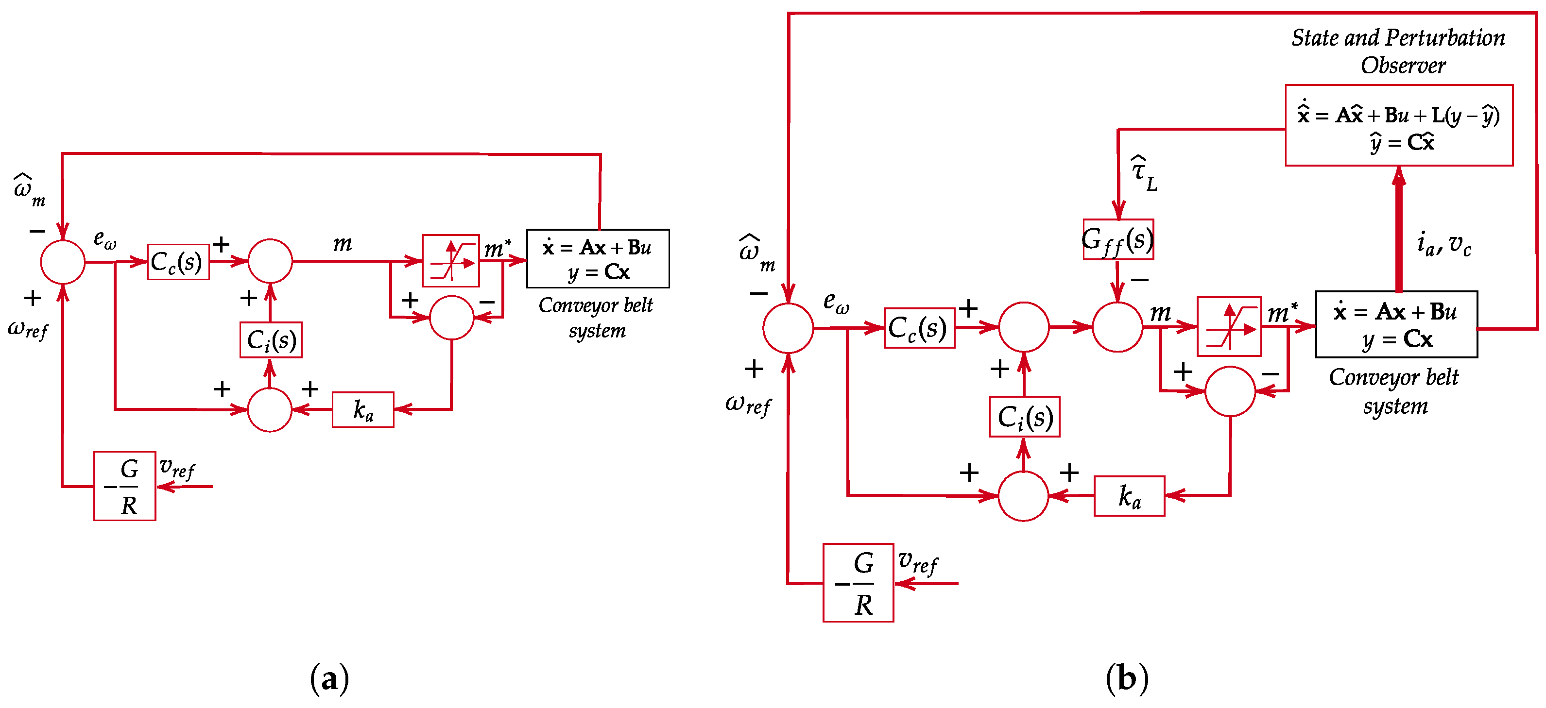
• A feedforward control scheme based on a low-order and causal filter is developed using frequency domain analysis, which is considered to reject external perturbations without using direct cancellation to compensate them;
• A state observer is proposed to estimate mechanical variables, such as angular velocity and torque load, and is used to develop a sensorless velocity regulator using only measurements of the DC motor’s armature current.

The main novelty of this work lies in the proposal of a new control scheme that integrates feedforward control and a state observer for regulating the DC motor drive of a bidirectional conveyor belt. Additionally, a deep performance analysis of the proposed control scheme is conducted through a series of tests designed to demonstrate how each component of the control scheme operates to improve the regulation of the DC motor.

This document is organized as follows: Section 1 introduces the application of DC motors, the problem formulation that defines the context of this study, and the contributions offered by this work. Section 3 describes the analytical models used to develop the control scheme for regulating these rotating machines, including state-space representation and transfer functions. This section also outlines the nominal parameters of each component within the mechatronic system and presents integral-based performance indices to assess the proposed control scheme and state observer. Section 4 details the design process of the control scheme, which combines conventional linear control theory with modern control techniques to create a sensorless control approach. In Section 5, the Discussion evaluates the components of the control scheme through tests that demonstrate the effectiveness of each internal element in regulating the motor. Lastly, Section 6 concludes with key insights and considerations drawn from the results.

2. Related Works

The specific application of the DC motor in this research is a challenge because of the typical operating conditions of the conveyor. The primary external perturbation affecting the system is the mechanical load imposed by the conveyor on the motor, which depends on factors such as the mass being transported. This load can be represented as a torque opposing the direction of the rotation of the motor’s rotor. Also, some nonlinearities associated with the mechanism can affect this, such as the dead zone and backlash. Another external perturbation influencing the performance of the DC motor is the DC voltage at the power terminals of the converter. Variations in this voltage can impact the amplitude of the armature voltage applied to the motor under specific operating conditions, potentially leading to the saturation of the high-frequency pulses driving the switches. These external perturbations can be managed using some schemes proposed in the literature and, in some cases, must be measured.

As previously mentioned, external perturbations can be compensated; however, in cases such as load torque, the sensors required for measurements are often expensive, increasing the overall cost of the control scheme. To reduce this economic burden, an external state observer can be implemented to estimate the mechanical variable. Understanding the behavior of this variable is crucial for designing an observer capable of accurately estimating it with minimal computational cost. In the present research work, the use of a feedforward scheme based on linear regulators is proposed to reject the negative effects produced by abrupt perturbations. The tuning of such regulators, developed using a conventional technique based on frequency analysis, is proposed.

Additionally, this state observer can estimate other variables, such as the angular velocity of the motor’s rotor, which are typically expensive to measure but essential for the development of the control scheme. Consequently, a control strategy relying solely on electrical measurements will be proposed, where mechanical variables will be estimated and utilized effectively.

The objective of this research is to develop a detailed analytical model of a mechatronic system that integrates a power converter, a permanent magnet DC motor, and a conveyor. Based on this model, a control scheme will be designed using conventional linear regulators and linear state observers to regulate the system according to a desired reference velocity.

The tuning process for the internal components of the control scheme will be carried out using both classical and modern control theories. Classical control theory will be employed to tune the regulator within the control scheme, while modern control theory will be utilized to design the linear state observer.

The validation of the proposed models will be conducted through simulations using a model developed in Simscape, a tool previously employed in related research as a reliable validator for various mechatronic systems, as described in [15].

3. Materials and Methods

3.1. Modeling Process

The first step in developing a control scheme to regulate a specific process is modeling that process. This design stage can be achieved through system identification, analytical modeling, or a combination of both. In this study, the analytical approach will be employed.

The system to be modeled consists of at least two subsystems: an electrical subsystem and a mechanical subsystem. To model the mechanical subsystem, Newton’s laws will be applied to describe the behavior of its components, while Kirchhoff’s laws will be used to model the electrical subsystem’s elements.

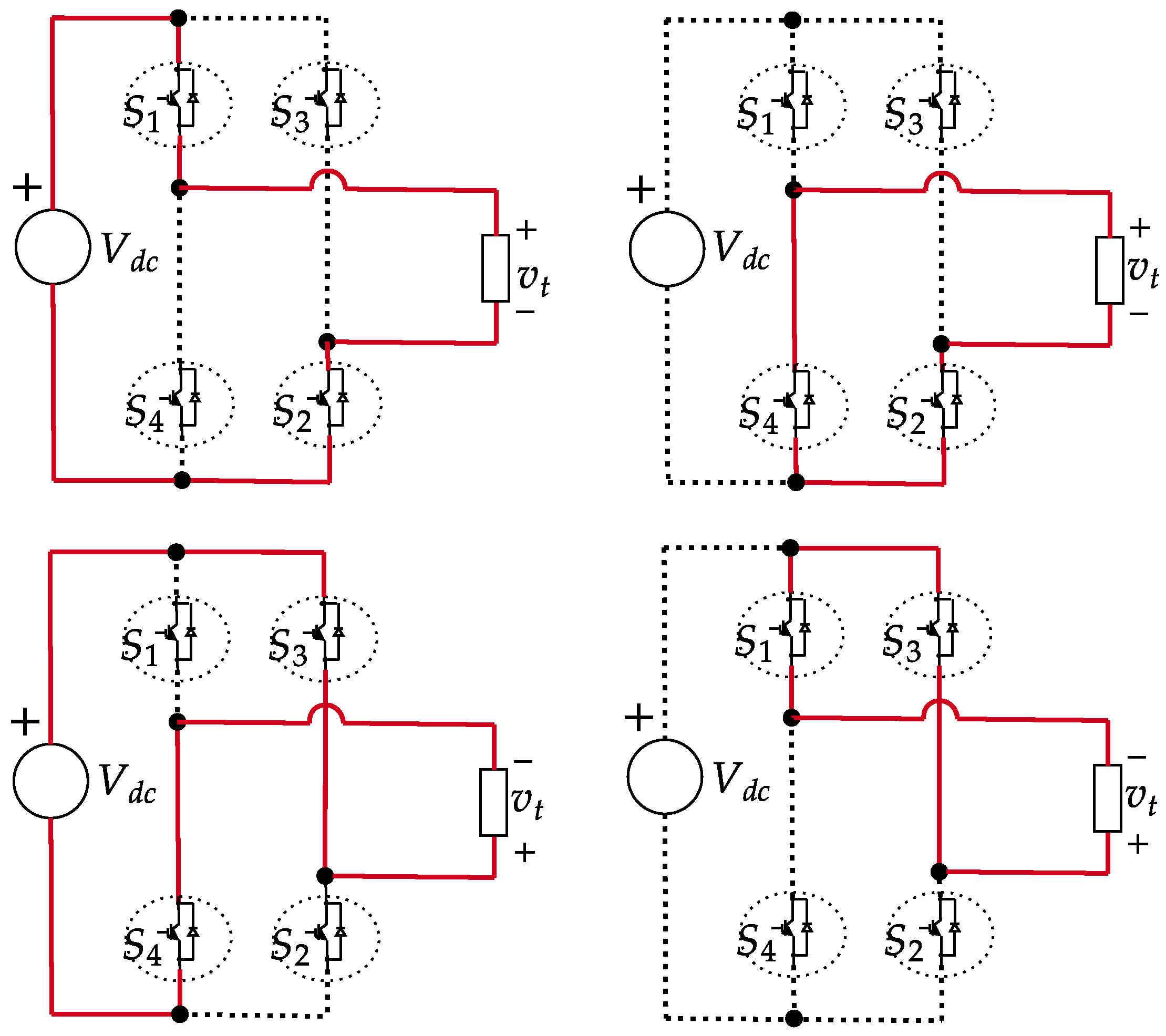
3.1.1. Model of the Power Converter

The first component of the electrical subsystem is the power converter. Its model will be developed based on the electrical circuits shown in Figure 1.

The equivalent circuit clearly highlights four functional blocks that characterize the behavior of the power converter. These blocks are identified as the DC link, switched block, ripple filter, and permanent magnet DC motor, each with a specific role.

The DC link, modeled as an ideal DC voltage source providing a voltage ($V_{dc}$), delivers the power necessary to ensure the motor’s rotor achieves the desired angular velocity. The switched block comprises semiconductor devices that facilitate the energy conversion process, allowing the DC motor to receive the appropriate voltage level for efficient operation.

The operational states of these switches are determined by the discrete variables $s_1$, $s_2$, $s_3$, and $s_4$, which can take values of either zero or one, depending on the desired effect over the output voltage ($v_t$). These signals typically exhibit high-frequency behavior. The operation of this block is depicted in Figure 2.

Considering the equivalent circuits presented above, truth

Table 1. Allowable combinations to manipulate the conversion process that occurs inside the full H-bridge power converter.

${\mathit{s}}_1$	${\mathit{s}}_2$	${\mathit{s}}_3\left({\overline{\mathit{s}}}_2\right)$	${\mathit{s}}_4\left({\overline{\mathit{s}}}_1\right)$	${\mathit{v}}_{\mathit{t}}$
1	1	0	0	$V_{dc}$
0	1	0	1	0
0	0	1	1	$-V_{dc}$
1	0	1	0	0

can be developed as follows:

As shown, the polarity of the output voltage can be reversed depending on the combination of switch states at any given time. This property enables the power converter to generate rotation in both directions for the motor’s rotor.

Another crucial aspect is that the pairs ($s_1,s_4$) and ($s_2,s_3$) cannot be activated simultaneously. These configurations are prohibited to prevent a short circuit in the DC link. Therefore, it is preferable to define $s_4$ as the complement of $s_1$ ($s_4=1-s_1$) and $s_3$ as the complement of $s_2$ ($s_3=1-s_2$). Each of these complementary signals is applied to a switching cell. In the case of this full H-bridge, two switching cells are controlled by the switching signals $s_1$ and $s_2$. In that case, all the possible configurations are given by the ones presented in Table 1.

The full H-bridge was considered to regulate the operation of the DC link because it is crucial in applications where the main DC voltage supplied by the main source cannot be changed according to the desired operation point of this machine or changes in the direction of the rotor’s movement are required. The DC motor can be supplied by the AC current through a rectifier, so in that case, the level of the rectified voltage cannot be regulated at will, and the use of a power converter is mandatory. Such regulation of the DC voltage level will be applied through the use of a PWM technique by the switching of inverter switches.

For the modeling process of the phenomena within the switched block, the following assumptions are made [16]:

• The semiconductor devices are considered as short circuits when they are in the on-state;
• The semiconductor devices are considered as open circuits when they are in the off-state;
• The dynamics associated with the switching transitions of the semiconductor devices are neglected.

Considering these properties and assumptions, the voltage at the switched block output is given by the next constitutive expression, which is similar to an XOR logic gate:

$$v_t=[s_1{s}_2-(1-s_1)(1-s_2)]V_{dc}=(s_1+s_2-1)V_{dc}.$$

(1)

An additional assumption is made to reduce the degrees of freedom in the power converter, where $s_1=s_2$. With this assumption, the previous constitutive expression can be rewritten as follows:

$$v_t=(2s_1-1)V_{dc}.$$

(2)

The ripple filter is designed to manage the high-frequency signals generated by the switching processes within the switched block. These high-frequency components, commonly referred to as harmonics, appear at the output terminal of the switched block. Harmonics can be detrimental to DC motors, as they may cause overheating in the machine, leading to negative effects on its performance and lifespan.

In the configuration shown in Figure 1, an LC filter is proposed to attenuate these harmonics, ensuring that the voltage applied to the armature terminals of the DC motor remains free from harmful high-frequency components. In the modeling process of this block, the DC motor is considered as a current source. Thus, the differential equations, capable of describing the dynamics of the power converter, are given as follows:

$$\begin{array}{c}L{\displaystyle \frac{d}{dt}}{i}_L=v_t-v_c\\ \\ C{\displaystyle \frac{d}{dt}}{v}_c=i_L-i_a\end{array}$$

(3)

Substituting (2) into (3), the following differential equations can be obtained:

$$\begin{array}{c}L{\displaystyle \frac{d}{dt}}{i}_L=(2s_1-1)V_{dc}-v_c\\ \\ C{\displaystyle \frac{d}{dt}}{v}_c=i_L-i_a\end{array}$$

(4)

The expressions presented above describe the switched model of the full H-bridge converter. This model is ideal for analyzing the effects of high-frequency switching on the performance of this type of device and is well suited for sizing the components of the ripple filter.

For the design of the control scheme, the switched model is not suitable because of the high computational cost associated with emulating the behavior of power-electronic-based systems. In such cases, average models are commonly used. These models focus on the fundamental component of the high-frequency pulses in the $s_1$ signal, which defines the system dynamics, while disregarding the higher-frequency components.

The obtainment of the average model of this converter requires the use of the average operator, which corresponds to the following expression:

$$\overline{x}={\int }_t^{t+T}xd\tau$$

(5)

where x represents the switched variable under analysis (assumed to exhibit periodic behavior), T is the period of such a signal, and $\overline{x}$ is the average variable corresponding to x. If $s_1$ is considered as a pulse train with a duty cycle of d, expression (5) can be modified as follows:

$$d={\int }_t^{t+T}{s}_{1}d\tau$$

(6)

Thus, in this case, the average model of the power converter is described by the following differential expressions, where a variable change is applied and corresponds to the expression $m=2d-1$ as follows:

$$\begin{array}{c}L{\displaystyle \frac{d}{dt}}{i}_L=m{V}_{dc}-v_c\\ C{\displaystyle \frac{d}{dt}}{v}_c=i_L-i_a\end{array}$$

(7)

The variable introduced by the previously proposed change is defined as the modulating signal, which is compared to a high-frequency signal to produce a specific high-frequency pulse train. It is important to note that $-1\le m\le 1$, requiring the use of a bipolar modulation technique [17].

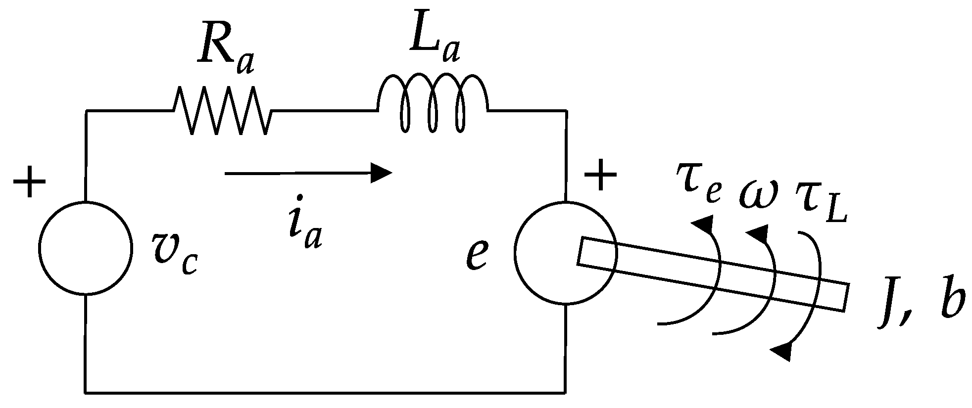
3.1.2. Model of the DC Motor

The permanent magnet DC motor is powered by the output voltage of the power converter. This rotating machine consists of two interconnected subsystems: electrical and mechanical. These subsystems are linked by the contra-electromotive force (e) and the electrical torque (${\tau }_e$), both of which are generated by the energy conversion process that occurs inside the motor.

This machine can be represented by the following equivalent circuit, where $R_a$ is the armature electrical resistance, $L_a$ is the armature inductance, J represents the inertia of the motor’s rotor under no-load conditions, and b corresponds to the dynamic friction associated with the rotor shaft. Additionally, $omega$ denotes the angular velocity of the rotor, ${\tau }_L$ represents the external torque imposed by the mechanical load the motor must drive, and $v_c$ is the voltage supplied by the power converter at the motor armature terminals.

In this type of machine, the relationships $e=k_{\omega }\omega$ and ${\tau }_e=k_i{i}_a$ hold, where $k_i$ is the torque constant, and $k_{\omega }$ is the back electromotive force constant [9]. The interaction between the two subsystems is governed by these equations, as they introduce mechanical variables to the electrical subsystem and electrical variables to the mechanical subsystem.These constants are determined by the electromagnetic properties and geometries of the magnet and the winding inside the DC motor.

Considering the electrical circuits presented in Figure 3 and neglecting certain nonlinearities within both the electrical and mechanical subsystems, the equations that describe the dynamics of this type of rotating machine are given as follows:

$$\begin{array}{c}{L}_a{\displaystyle \frac{d}{dt}}{i}_a=v_c-i_a{R}_a-k_{\omega }\omega \\ \\ J{\displaystyle \frac{d}{dt}}\omega =k_i{i}_a-{\tau }_L-b\omega \end{array}$$

(8)

From these expressions, it can be observed that the DC motor interacts with the power converter through the variables $i_a$ and $v_c$, in which $v_c$ acts as an external input, and $i_a$ serves as the output injected into the model described by the equations in (7).

Both sets of differential equations presented in (7) and (8) can be combined to formulate a state-space representation that characterizes the dynamics of the combined power converter and DC motor system. This state-space representation is expressed through the following matrix equation:

$${\dot{\mathbf{x}}}_M={\mathbf{A}}_M{\mathbf{x}}_M+{\mathbf{B}}_M{\mathbf{u}}_M$$

(9)

where ${\mathbf{x}}_M={\left[\begin{array}{cccc}{i}_L& v_c& i_a& \omega \end{array}\right]}^T$ is the state vector, ${\mathbf{u}}_M={\left[\begin{array}{cc}m& {\tau }_L\end{array}\right]}^T$ is the input vector, and ${\mathbf{A}}_M$ and ${\mathbf{B}}_M$ are the state and input matrices, respectively. These matrices are defined as follows:

$$\begin{array}{c}{\mathbf{A}}_M=\left[\begin{array}{cccc}0& -{\displaystyle \frac{1}{L}}& 0& 0\\ {\displaystyle \frac{1}{C}}& 0& -{\displaystyle \frac{1}{C}}& 0\\ 0& {\displaystyle \frac{1}{L_a}}& -{\displaystyle \frac{R_a}{L_a}}& -{\displaystyle \frac{k_{\omega }}{L_a}}\\ 0& 0& {\displaystyle \frac{k_i}{J}}& -{\displaystyle \frac{b}{J}}\end{array}\right]{\mathbf{B}}_M=\left[\begin{array}{cc}{\displaystyle \frac{V_{dc}}{L}}& 0\\ 0& 0\\ 0& 0\\ 0& -{\displaystyle \frac{1}{J}}\end{array}\right]\end{array}$$

(10)

As $V_{dc}$ is assumed to remain constant, the state-space representation describes a linear system. Consequently, transfer functions can be derived to characterize the interactions between the external inputs and the angular velocity of the DC motor.

$$\begin{array}{c}{\displaystyle \frac{\omega \left(s\right)}{m\left(s\right)}}=G_1\left(s\right)={\displaystyle \frac{V_{dc}{k}_i}{CJL{L}_a{s}^4+CL(J{R}_a+L_{a}b)s^3+CL(R_{a}b+k_e{k}_i)s^2+(J{R}_a+Lb)s+Rab+k_e{k}_i}}\\ \\ {\displaystyle \frac{\omega \left(s\right)}{{\tau }_L\left(s\right)}}=G_2\left(s\right)=-{\displaystyle \frac{CL{L}_a{s}^3+CL{R}_a{s}^2+(L+L_a)s+R_a}{CJL{L}_a{s}^4+CL(J{R}_a+L_{a}b)s^3+CL(R_{a}b+k_e{k}_i)s^2+(J{R}_a+Lb)s+Rab+k_e{k}_i}}\end{array}$$

(11)

These transfer functions are obtained using the following matrix expression:

$$G\left(s\right)={\mathbf{C}}_M{(s\mathbf{I}-{\mathbf{A}}_M)}^{-1}{\mathbf{B}}_M,$$

(12)

where ${\mathbf{C}}_M$ is the output matrix, defined as ${\mathbf{C}}_M=\left[\begin{array}{cccc}0& 0& 0& 1\end{array}\right]$, and $\mathbf{I}$ is the identity matrix with dimensions matching the number of states used to describe the system. It is important to note that the transfer function ($G_1\left(s\right)$) has no zeros and is of the fourth order, while $G_2\left(s\right)$ has three zeros and a negative gain. Using these transfer functions, the following block diagram can be structured (Figure 4).

These transfer functions and the block diagram will serve as the foundation for designing the control scheme intended to regulate the operation of the bidirectional conveyor’s actuator.

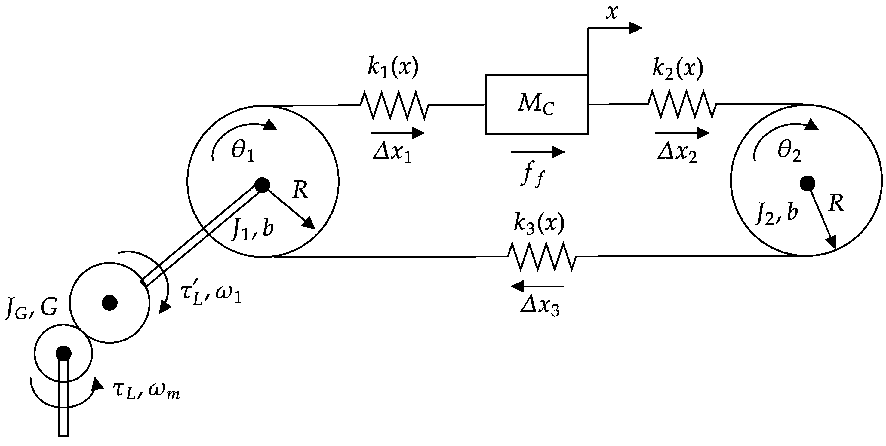
3.1.3. Space-State-Based Model of the Conveyor

Conveyor systems are used for several applications, such as in agricultural machines, electric generators, robotic arms, machine tools, and textile machines [18]. They are straightforward, lightweight, and cost-effective power transmission systems that convert rotational to translational movement. In this case, the conveyor is regarded as a belt designed to transport sugarcane from one location to another for industrial processing.

The previously modeled DC motor will be used to drive this conveyor belt in both directions. To analyze the behavior of the complete system—comprising the power converter, DC motor and conveyor—the development of an analytical model exclusively for the conveyor is required. This model will demonstrate the linear motion of the conveyor in response to the torque applied by the motor’s rotor. The conveyor to be modeled is illustrated in Figure 5 and is commonly denoted as the three-mass model [19].

This representation consists of a timing belt, a carriage, and two pulleys, identified as the driving and driven pulleys [20]. These pulleys are responsible for stretching the conveyor belt and transmitting force from the driving pulley to the carriage, which represents the mass being transported along the conveyor. The conveyor model exhibits highly coupled and nonlinear dynamics, with the added complexity of exogenous disturbances [19].

In such a figure, $J_1$, ${\theta }_1$, and ${\omega }_1$ represent the inertia, angular displacement, and angular velocity associated with the driving pulley, while $J_2$, ${\theta }_2$, and ${\omega }_2$ correspond to the inertia, angular displacement, and angular velocity of the driven pulley. Both pulleys share the same radius, R, and viscous damping coefficient, $b_c$. The torque (${\tau }_L$) accounts for the load exerted by the entire conveyor system on the rotor of the DC motor. $J_G$ represents the inertia of the reduction gearbox, and G denotes its gear ratio.

The elastic coefficients ($k_1\left(x\right)$, $k_2\left(x\right)$, and $k_3\left(x\right)$) characterize the stiffness of the conveyor [19]. $\Delta x_1$, $\Delta x_2$, and $\Delta x_3$ represent the deflection that characterizes these equivalent springs. Finally, $M_c$ is the mass of the carriage, which moves along the conveyor and is described by its position (x) and velocity (v). As slip is not considered in the movement of the conveyor and the carriage, $\Delta x_1=\Delta x_2=\Delta x_3=0$, and $v=R{\omega }_1=R{\omega }_2$.

The mass of the sugarcane transported along the conveyor belt, denoted as $M_{sc}$, is given by $M_{sc}=M_c-M_o$, where $M_o$ represents the mass of the conveyor belt. The dynamics of the sugarcane’s mass can be modeled as a consequence of the input and output mass fluxes [21]. These fluxes can be described as follows:

$$F_M(t,x)=A_e{h}_e(t,x)v\left(t\right){\rho }_e$$

(13)

where $A_e$ represents the width of the conveyor belt, and $h_e$ denotes the height of the sugarcane profile. This height varies over time and depends on the position at which the variable is measured. For this analysis, the height is considered at the beginning and the end of the conveyor belt. Finally, ${\rho }_e$ represents the density of the sugarcane on the conveyor belt. If $F_{Mi}$ and $h_{ei}$ are considered as the input mass flux and profile height and $F_{Mo}$ and $h_{eo}$ are considered as the output mass flux, the dynamics associated with the sugarcane’s mass are given as follows:

$${\displaystyle \frac{d}{dt}}{M}_{sc}=F_{Mi}-F_{Mo}=A_e{\rho }_e(h_{ei}-h_{eo})v$$

(14)

where $h_{eo}$ directly depends on $h_{io}$, with this relationship being governed by a variable transport delay. This delay represents how sugarcane is introduced to the conveyor belt and subsequently exits it. In the present research work, both heights are considered as exogenous inputs.

In the expression above, L is the length of the conveyor belt. To model this mechanical system, the following assumptions are considered [19]:

• The link between the motor shaft and the driving pulley is rigid;
• No backlash is present in the system;
• The belt can be modeled by a constant mass ($M_o$);
• The density of sugarcane’s mass is maintained as constant along the conveyor belt.

Considering all the aforementioned assumptions, the conveyor’s structure illustrated in Figure 5, and Newton’s laws, the following third-order mathematical model is presented [18,21,22]:

$$\begin{array}{c}{\displaystyle \frac{d}{dt}}{M}_{sc}=R{A}_e{\rho }_e(h_{ei}-h_{eo}){\omega }_1\\ J_{eq}{\displaystyle \frac{d}{dt}}{\omega }_1=-G{\tau }_L-2b_c{\omega }_1\end{array}$$

(15)

where $J_{eq}=R^2(M_{sc}+M_0)+G^2{J}_G+J_1+J_2$. These differential equations can be integrated with the previously established ones to develop a unified model, enabling accurate emulation of the system comprising the power converter, DC motor, and conveyor belt.

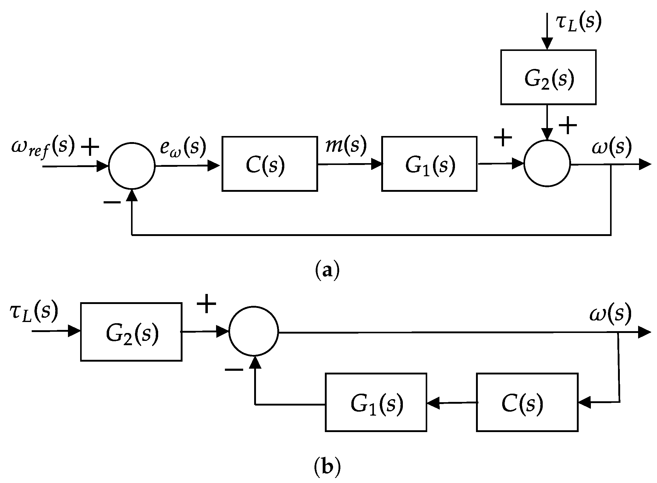
3.1.4. Unified Analytical Model

To unify the previously modeled dynamics, it is necessary to express the dynamics of the DC motor in the reference frame corresponding to the movement of the conveyor’s carriage. The following expression will be taken into account to perform this conversion process, where $G>1$ when a velocity reductor is used to couple the conveyor with the DC motor:

$$\begin{array}{cc}{\displaystyle \frac{{\tau }_m}{{\tau }_m^{\prime }}}=-{\displaystyle \frac{1}{G}}& {\displaystyle \frac{{\omega }_m}{{\omega }_1}}=-G\end{array}$$

(16)

Based on the previous constitutive expressions, the following differential equations can be derived to describe the motor’s dynamics:

$$\begin{array}{c}{L}_a{\displaystyle \frac{d}{dt}}{i}_a=v_c-i_a{R}_a+G{k}_{\omega }{\omega }_1\\ \\ -GJ{\displaystyle \frac{d}{dt}}{\omega }_1=k_i{i}_a-{\tau }_L+Gb{\omega }_1\end{array}$$

(17)

To solve for ${\tau }_L$ in the dynamics that characterized the conveyor’s dynamics, we obtain that

$${\tau }_L=-{\displaystyle \frac{J_{eq}\frac{d}{dt}{\omega }_1+2b_c{\omega }_1}{G}}$$

(18)

Substituting this expression into the equation that describes the dynamics of the mechanical subsystem, the entire system can be modeled by the following set of first-order differential equations:

$$\begin{array}{c}L{\displaystyle \frac{d}{dt}}{i}_L=m{V}_{dc}-v_c\\ \\ C{\displaystyle \frac{d}{dt}}{v}_c=i_L-i_a\\ \\ L_a{\displaystyle \frac{d}{dt}}{i}_a=v_c-i_a{R}_a+G{k}_{\omega }{\omega }_1\\ \\ (G^{2}J+J_{eq}){\displaystyle \frac{d}{dt}}{\omega }_1=-G{k}_i{i}_a-(G^{2}b+2b_c){\omega }_1\\ \\ {\displaystyle \frac{d}{dt}}{M}_{sc}=R{A}_e{\rho }_e(h_{ei}-h_{eo}){\omega }_1\end{array}$$

(19)

As can be seen, this is a fifth-order model, in which three states are electrical variables ($i_L$, $v_c$, and $i_a$), one is a mechanical variable (which is represented by ${\omega }_1$), and the last one is the sugarcane’s mass ($M_{sc}$). This model has three external inputs, which are m, $h_{ei}$, and $h_{eo}$, if it is considered that $V_{dc}$ is constant. The first variable is considered as a manipulable input, while the latter two are treated as external perturbations. These differential equations describe a nonlinear dynamic system because of the presence of products involving time-dependent variables. Additionally, some functions depend on the product of state variables and inputs.

If the following state vector $\mathbf{x}={\left[i_L{v}_c{i}_a{\omega }_1{M}_{sc}\right]}^T$ and input vector $\mathbf{u}={\left[m{h}_{ei}{h}_{eo}\right]}^T$ are defined, the state and input matrices are given by the following ones:

$$\begin{array}{c}\mathbf{A}=\left[\begin{array}{ccccc}0& -{\displaystyle \frac{1}{L}}& 0& 0& 0\\ {\displaystyle \frac{1}{C}}& 0& -{\displaystyle \frac{1}{C}}& 0& 0\\ 0& {\displaystyle \frac{1}{L_a}}& -{\displaystyle \frac{R_a}{L_a}}& {\displaystyle \frac{G{k}_{\omega }}{L_a}}& 0\\ 0& 0& -{\displaystyle \frac{G{k}_i}{G^2(J+J_G)+R^2(M_{sc}+M_0)+J_1+J_2}}& -{\displaystyle \frac{G^{2}b+2b_c}{G^2(J+J_G)+R^2(M_{sc}+M_0)+J_1+J_2}}& 0\\ 0& 0& 0& R{A}_e{\rho }_e(h_{ei}-h_{eo})& 0\end{array}\right]\\ \\ \mathbf{B}=\left[\begin{array}{ccc}{\displaystyle \frac{V_{dc}}{L}}& 0& 0\\ 0& 0& 0\\ 0& 0& 0\\ 0& 0& 0\\ 0& 0& 0\end{array}\right]\end{array}$$

(20)

The present research aims to regulate the velocity at which the conveyor belt transports the sugarcane. Accordingly, the output of the model is defined by the following matrix equation: $y=\mathbf{C}\mathbf{x}$, where $\mathbf{C}={\left[0000R\right]}^T$. This state-space representation model will be used to evaluate the proposed control scheme for regulating the angular velocity of the DC motor’s rotor. The load torque acting on the rotor is determined by the effect of the conveyor system, which is accurately incorporated into the previously defined state-space representation.

3.2. Case Study Parameters

3.2.1. Conveyor Belt

The selection of parameters influencing the dynamics of the conveyor belt is based on pre-established values proposed in previous research studies and is specifically tailored to the stationary operational conditions of the mechanical system. The first condition derived from the aforementioned differential equations pertains to the dynamics of the sugarcane’s mass. In this case, it is required that both heights are equal to ensure that $M_c$ remains constant, even if ${\omega }_1\ne 0$.

It is considered that the conveyor belt has the following dimensions: $A=0.3$ m and $L=4$ m. It is considered that at a nominal capacity, the conveyor is transporting around a sugarcane profile with a mean height of $h=0.25$ m. In [21], the authors considered a volumetric density of $\rho =400{\displaystyle \frac{\mathrm{kg}}{{\mathrm{m}}^3}}$. In that case, ${\widehat{M}}_{sc}=120$ kg when it is considered that $v\approx 1{\displaystyle \frac{\mathrm{m}}{\mathrm{s}}}$. The parameters used to describe the conveyor are presented in

Table 2. Parameters used to configure the conveyor belt.

Parameter	Unit	Value
G	-	18
$J_G$	kg·m2	1 × 10−4
$J_1$	kg·m2	1 × 10−2
$J_2$	kg·m2	1 × 10−2
R	m	0.15
$b_c$	${\displaystyle \frac{\mathrm{kg}}{\mathrm{s}}}$	2.5
$M_o$	kg	40
L	m	4
A	m	0.3
${\rho }_e$	${\displaystyle \frac{\mathrm{kg}}{{\mathrm{m}}^3}}$	400
${\overline{h}}_{ei}$	m	0.25
${\overline{h}}_{eo}$	m	0.25
$\overline{v}$	${\displaystyle \frac{\mathrm{m}}{\mathrm{s}}}$	1
${\overline{M}}_{sc}$	kg	120

.

3.2.2. DC Motor

The permanent magnet DC motor considered for this system is characterized by the parameter values presented in

Table 3. Parameters used to configure the permanent magnet DC motor.

Parameter	Unit	Value
J	$\mathrm{kg}·{\mathrm{m}}^2$	6.96 × 10−3
b	${\displaystyle \frac{\mathrm{N}·\mathrm{m}·\mathrm{s}}{\mathrm{rad}}}$	1.73 × 10−3
$V_n$	V	90
$k_i$	${\displaystyle \frac{\mathrm{N}·\mathrm{m}}{\mathrm{A}}}$	0.35
$k_{\omega }$	${\displaystyle \frac{\mathrm{V}·\mathrm{s}}{\mathrm{rad}}}$	0.35
$L_a$	mH	28.44
$R_a$	$\Omega$	1.27

.

3.2.3. Ripple Filter

The values for the ripple filter were selected following the criteria outlined by Antritter et al. in [23]. The frequency of the PWM voltage generated by the power inverter is 4.5 kHz. This value was chosen to generate a pulse sequence fast enough to ensure that such high-frequency pulses do not affect the performance of a DC motor with a non-DC voltage component. Considering such a value of the switching frequency, the nominal values of the internal components of the proposed power converter’s ripple filter are chosen. The coil inductance was chosen to attenuate the current ripple in $i_L$ caused by the high-frequency switching used to regulate the operation of the DC motor. It is important to note that excessively high inductance values were avoided to prevent increased ohmic losses, which would reduce the efficiency of the conveyor’s actuator. The capacitor was sized to create a low-pass filter capable of mitigating high-frequency voltage harmonics introduced by the PWM technique. Based on these criteria, the following values were chosen: L = 4.7 mH, and C = 47 $\mathsf{\mu }$F.

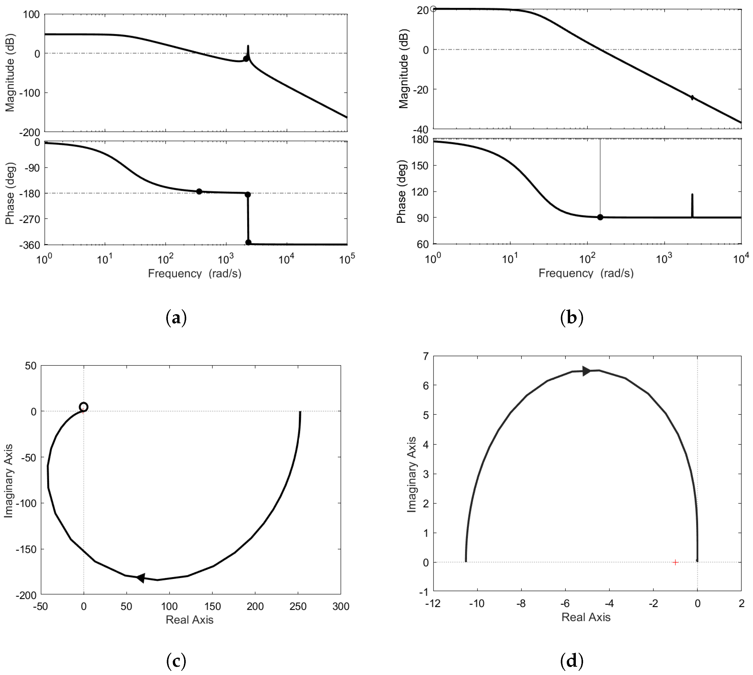
3.3. Characteristics of the Transfer-Function-Based Models

Considering these values, the transfer functions given in (11) have the following numerical values:

$$\begin{array}{c}{G}_1\left(s\right)={\displaystyle \frac{28.8}{4.3725e-11s^4+1.8558e-09s^3+2.3068e-04s^2+0.0084s+0.1141}}\\ \\ G_2\left(s\right)=-{\displaystyle \frac{6.2824e-09s^3+2.6508e-07s^2+0.0331s+1.2}{4.3725e-11s^4+1.8558e-09s^3+2.3068e-04s^2+0.0084s+0.1141}}\end{array}$$

(21)

The frequency response of the previously obtained models is presented in Figure 6, which includes Bode diagrams and a Nyquist plot to characterize the behavior of the conveyor’s actuator in the frequency domain.

These transfer functions exhibit different minimum bandwidths. $G_1\left(s\right)$ has a minimum bandwidth of 358 rad/s. Therefore, the proposed control scheme for regulating the angular velocity of the rotating machine must operate below this limit. Additionally, a resonance peak occurs at 2300 rad/s, which is likely strongly correlated with the ripple filter dynamics, as it was modeled using ideal components. At this resonance peak, a sudden phase shift is observed, which could negatively impact the dynamics of the closed-loop system intended to regulate the operation of the DC motor.

It is necessary to propose a control scheme capable of avoiding encirclement around the point $(-1,0)$ in the Nyquist plot. This approach ensures a stable closed-loop dynamic, as the open-loop poles of $G_1\left(s\right)$ are all located in the stable region, as shown in Figure 7, specifically in Figure 7a,c.

For the transfer function $G_2\left(s\right)$, the bandwidth is 147 rad/s, which is lower than that of $G_1\left(s\right)$. This bandwidth is significant because it represents the frequency range in which the load torque may negatively impact the dynamics of the conveyor’s actuator. Figure 7b,d shows the locations of the open-loop zeros and poles characterizing the transfer function ($G_2\left(s\right)$).

3.4. Emulation of the System Using the Space-State-Based Model

Figure 8 illustrates the behavior of the complete system described by the state-space representation introduced in (20). The figure displays both the linear velocity of the conveyor and the armature current of the DC motor in response to changes in the applied modulating signal, and the mass transported over the conveyor behaves as a constant.

Sudden changes in the modulating signals result in overcurrents in the armature circuit of the DC motor. This behavior is undesirable, as it can lead to damage to the circuitry of the motor or even complete failure. Another noticeable result is the fact that the selected motor is capable of generating the desired linear motion of the conveyor.

Therefore, it is necessary to implement a control scheme capable of accurately regulating the angular velocity of the motor’s rotor to meet the required linear velocity while ensuring that changes in the modulating signals prevent the occurrence of hazardous overcurrents.

3.5. Index Criteria Used

The evaluation process developed to assess the impact of applying the proposed scheme will be quantified by integral-index-based criteria. These criteria are based on analyzing the behavior of the error between the reference applied and the output intended to be regulated. They are usually denoted as integral-based error indices [24].

Some of these indices are the integral absolute error (IAE) and integral square error (ISE) [25]. The IAE is an index used to measure the total error related to the behavior of a controlled system or an estimation process over the entire test duration. This criterion is based on analyzing the absolute value of the error, making it indifferent to the error’s sign. This characteristic makes it an excellent metric for quantifying the overall error in a system. This index is given by the following expression, which is a discrete version of the IAE criterion:

$$IAE={\displaystyle \frac{1}{nA}}\sum _{i=0}^n(r_i-y_i)$$

(22)

In this definition, n represents the number of data points considered during the evaluation process, A is the reference magnitude applied over a specific period, $r_i\left(t\right)$ is the reference signal within the control loop, and $y_i\left(t\right)$ is the actual output of the process. Consequently, $e_i\left(t\right)=r_i\left(t\right)-y_i\left(t\right)$ represents the actual error present within the control loop. This index is normalized with respect to both the magnitude and number of data points, which is advantageous for conducting a critical and objective analysis.

The ISE criterion is valuable to assess how large the error produced along the operation of the controlled process is. The expression used to quantify it is given as follows:

$$ISE={\displaystyle \frac{1}{nA}}\sum _{i=0}^n{e}_i^2$$

(23)

The main difference between this criterion and the IAE lies in the fact that the error is squared. This modification places greater emphasis on larger deviations from the reference, penalizing them more heavily than smaller errors. As a result, this index is particularly useful for evaluating whether a controlled process exhibits oscillatory behavior or overshoots. Like the IAE, this index will also be normalized to ensure consistency in the analysis.

The impacts of external perturbations on the modulating signals generated by each controller in the proposed scheme will be quantified using IAE- and ISE-based indices. These are defined by the following expressions:

$${IAE}_m={\displaystyle \frac{1}{n\overline{m}}}\sum _{i=0}^n(m_i-\overline{m}){ISE}_m={\displaystyle \frac{1}{n\overline{m}}}\sum _{i=0}^n{(m_i-\overline{m})}^2$$

(24)

In these expressions, $\overline{u}$ denotes the average value of the command signal produced by the controller in response to a specific reference input within the control scheme, $m_i$ is the ith value associated with the modulating signal applied; meanwhile, $\overline{m}$ is the mean value of all the modulating signals generated by the controller. The modified indices are defined to quantify, in a normalized manner, the magnitude of the variations in the command signal, thereby effectively emphasizing the impacts of such perturbations.

4. Results

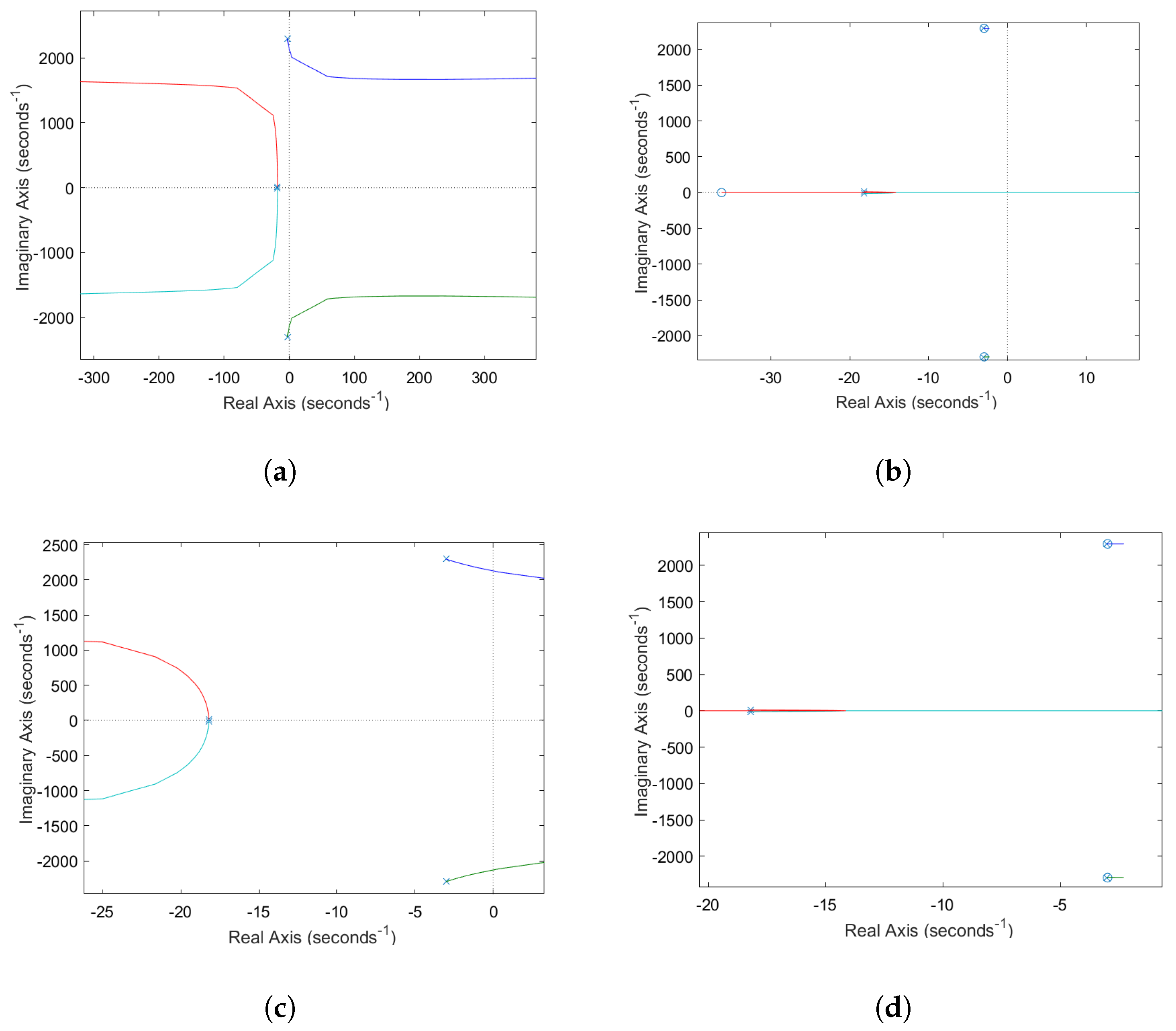
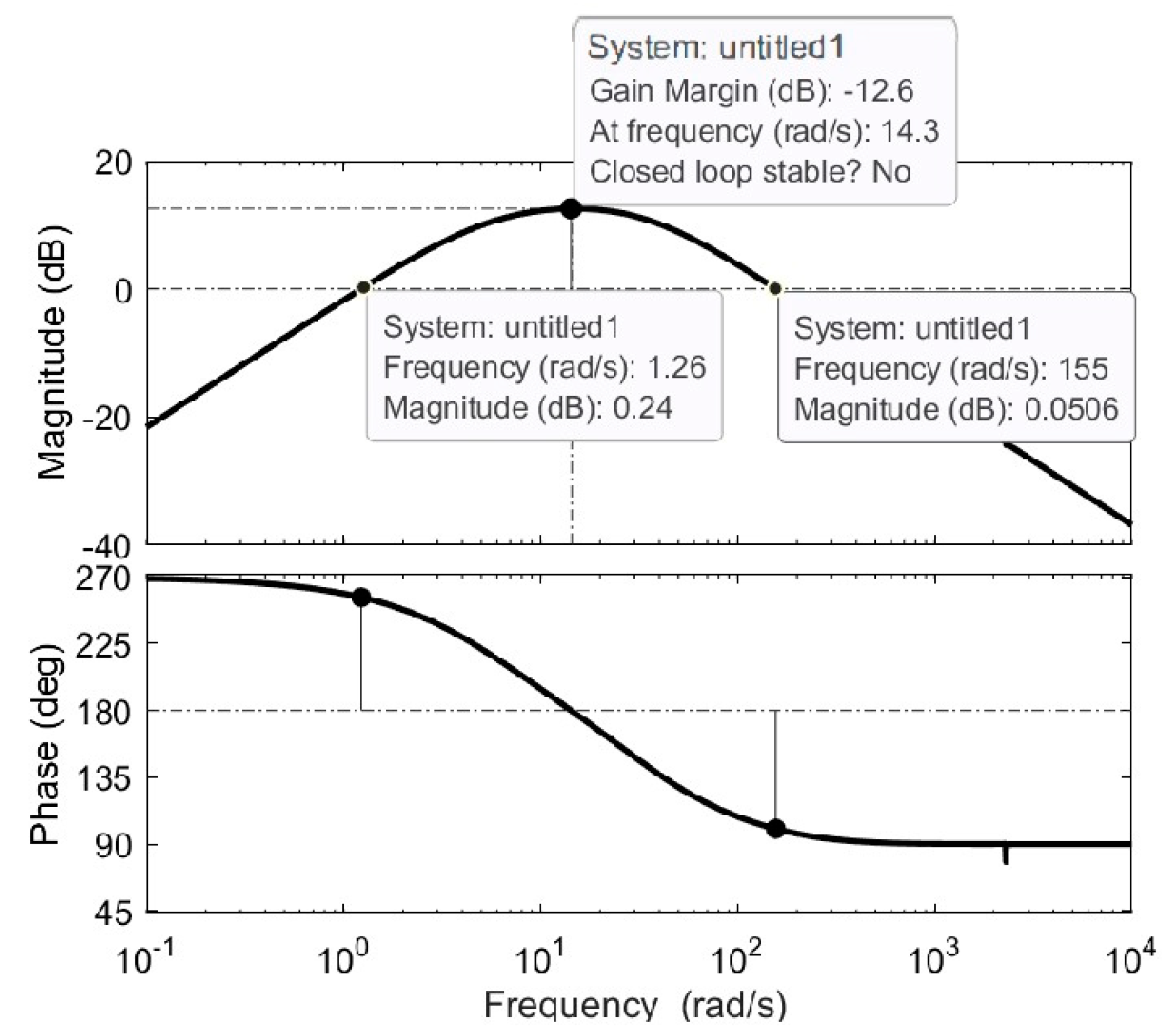
4.1. Design of the Regulator of the Control Scheme

The controller selected for regulating the angular velocity of the motor’s rotor is designed based on the transfer function ($G_1\left(s\right)$) presented in (21). For the selection of such a component, it is considered that the load torque is null the first time. After the selection of this controller, the effect of the external perturbation over the closed loop will be assessed using the classical theory of control.

As previously emphasized, the corrective actions generated by the controller regulating the process characterized by the transfer function ($G_1\left(s\right)$) must be smooth to prevent the occurrence of overcurrents. Achieving this requires tuning a linear controller that ensures robust stability margins while avoiding underdamped dynamics in the closed-loop configuration. Additionally, it is desirable for the closed-loop system to accurately track the imposed reference for the angular velocity.

The first time, the following regulator is proposed, which corresponds to a PI controller:

$$C\left(s\right)=0.5{\displaystyle \frac{0.1s+1}{s}}$$

(25)

The integral action of the proposed $PI$ controller is intended to ensure the accurate tracking of the constant reference signal applied at the loop’s input when the system operates under steady-state conditions. The proportional action is designed to achieve the fast convergence of the error between the actual output and the applied reference to zero. Additionally, a gain is introduced to adjust the closed-loop’s bandwidth, allowing for improved dynamic performance.

The Bode diagram corresponding to the open-loop configuration of the controlled angular-velocity dynamics is shown in Figure 9. This frequency response indicates a gain margin of 42.1 dB (as shown in Figure 9a) and a phase margin of 19.6°. Although the gain margin suggests a robust closed-loop configuration, the phase margin is insufficient, failing to guarantee robustness. The bandwidth of this dynamic system is 78.2 rad/s (displayed in Figure 9b), which is less than a decade below the inherent bandwidth of the conveyor’s actuator.

To overcome the low-phase margin obtained before, a lead compensator is proposed together with the PI presented before [26]. In that case, the whole angular velocity regulator is given by the following transfer function:

$$C\left(s\right)=0.05{\displaystyle \frac{0.1s+1}{s}}{\displaystyle \frac{0.5s+1}{0.003s+1}}$$

(26)

The Bode diagram associated with the use of this controller to regulate such dynamics is presented in the following Figure 10.

A gain margin of 20.7 dB and a phase margin of 101° are obtained, both of which indicate that the controlled dynamics are robust. Additionally, the high-phase margin corresponds to an overdamped dynamic response, which is desirable to prevent overcurrents during changes in the operating conditions of the conveyor’s actuator. The bandwidth of this dynamic system is 30.5 rad/s, approximately a decade below the inherent bandwidth of the actuator. These properties ensure that the command signals generated by the controller are not attenuated by the dynamics’ actuator. In Figure 11, the Nyquist plot related to such controlled dynamics is presented.

The Nyquist plot shows that the controlled system dynamics are far from the critical point (−1, 0). However, at certain frequency values, the plot resides in the positive real semi-plane of the diagram. This characteristic could result in underdamped behavior under specific operating conditions. To mitigate this, the reference applied to the controlled dynamics may need to be restricted, preventing the activation of such a behavior and avoiding high levels of armature current in the DC motor.

4.2. Analysis of the Sensibility Transfer Function

It is necessary to analyze the effect of the proposed controller on mitigating the influence of external disturbances, such as ${\tau }_L\left(s\right)$. For this purpose, block diagrams are presented in Figure 12, illustrating the developed control scheme and the structure required to evaluate the disturbance rejection capabilities of the proposed approach.

The block diagram shown in Figure 12b is obtained by setting ${\omega }_{ref}=0$ and adjusting the resulting scheme accordingly. In the case of the block diagram presented in such a figure, the sensitivity transfer function is given by the following expression [27]:

$$S\left(s\right)={\displaystyle \frac{1}{1+G_1\left(s\right)C\left(s\right)}}$$

(27)

The frequency response of this transfer function is shown in the Bode diagram presented in Figure 13. As a high-pass filter, the sensitivity transfer function effectively attenuates low-frequency external disturbances. However, a notable drawback is that the control scheme does not sufficiently reject high-frequency components of these disturbances. The disturbance rejection capability of the control scheme weakens at approximately 86.2 rad/s. This frequency range should be analyzed in the transfer function ($G_2\left(s\right)$) to evaluate the impact of the load torque on the angular velocity of the motor’s rotor.

It is important to note that as previously analyzed, the bandwidth associated with $G_2\left(s\right)$ exceeds the frequency range where the sensitivity rejection capability of the transfer function weakens. As a result, the load torque can influence the angular velocity within a certain frequency range. Figure 14 shows the frequency response of the transfer function (${\displaystyle \frac{\omega \left(s\right)}{{\tau }_L\left(s\right)}}$), considering the loop configured by the previously proposed controller. This transfer function is defined by the following expression:

$${\displaystyle \frac{\omega \left(s\right)}{{\tau }_L\left(s\right)}}={\displaystyle \frac{G_2\left(s\right)}{S\left(s\right)}}$$

(28)

It is observed that the load torque can affect the angular-velocity dynamics in the frequency range from 1.26 rad/s to 155 rad/s. This range is significant because within these frequencies, the impact of the load torque on the angular-velocity dynamics is amplified, which is undesirable because the load torque is an external disturbance. It is important to note that at low frequencies and under steady-state operational conditions, the load torque is strongly attenuated, having the minimal effect on the ability of the proposed control scheme to regulate the angular velocity. The maximum gain is achieved at a frequency of 14.3 rad/s, with a value of 12.6 dB.

The behavior analyzed previously must be corrected by implementing a compensation method. In this research, a feedforward scheme is proposed, which has been used in various applications that require this type of compensation, such as in [28].

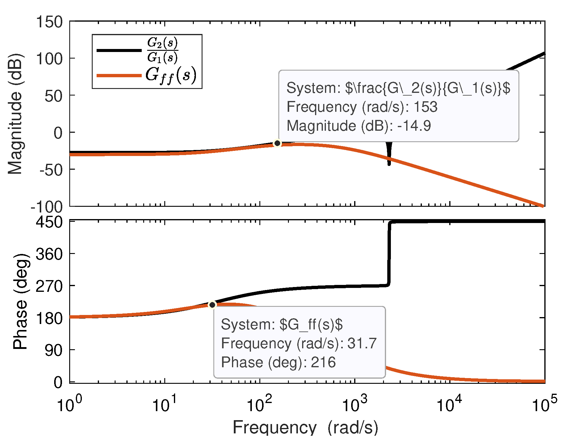
4.3. Feedforward Control Scheme’s Design

Figure 15 presents the block diagram corresponding to the use of a feedforward compensation scheme. In Figure 15a, the entire control scheme is shown, while Figure 15b presents the equivalent block diagram representing the dynamic behavior of the angular velocity caused solely by a load torque applied to the motor’s rotor.

In the feedforward-based control scheme, $G_{ff}\left(s\right)$ represents the compensator used to attenuate the negative effects produced by the load torque. For the analysis developed in this subsection, it is assumed that this load torque is known through measurements obtained from sensors. The ideal feedforward compensator satisfies the following condition, as it can be derived from the block diagram presented in Figure 15b:

$$G_{ff}\left(s\right)={\displaystyle \frac{G_2\left(s\right)}{G_1\left(s\right)}}$$

(29)

Figure 16 presents the Bode diagram corresponding to the frequency response of the ideal feedforward compensator. This ideal compensator is not feasible to implement because it is non-causal, as the number of zeros in $G_2\left(s\right)$ exceeds the number of zeros in $G_1\left(s\right)$. This property can be inferred from the frequency response, particularly from the behavior of the magnitude at high frequencies.

Therefore, it is necessary to propose a compensator that approximates the ideal $G_{ff}\left(s\right)$ within the frequency range where the impact of load torque on the angular-velocity dynamics of the DC motor is amplified. So, the following compensator is proposed:

$$G_{ff}\left(s\right)=-0.03{\displaystyle \frac{0.042s+1}{1.4e-8s^3+2.15e-5s^2+0.0096s+1}}$$

(30)

Figure 17 compares the frequency responses of the proposed compensator and the ideal compensator. The magnitudes of both responses are nearly identical from the low-frequency range up to approximately 153 rad/s. This result aligns with expectations for achieving the effective attenuation of the load torque in the originally designed closed-loop system.

However, the phase responses match over a narrower frequency range compared to that of the magnitude of the responses. The high absolute order selected for designing this compensator is motivated by the need to align with the resonance frequency observed in the frequency response of the ideal compensator at a high frequency response.

Figure 18 shows the frequency response of the equivalent transfer function ($G_2\left(s\right)$) after applying the feedforward compensator. When compared to the Bode diagram in Figure 6b, several differences can be observed, including a decrease in the low-frequency magnitude and a reduction in bandwidth. Both changes are beneficial to increase the capability of the control scheme to reject the existence of such external perturbations.

Figure 19 compares the transfer functions (${\displaystyle \frac{\omega \left(s\right)}{{\tau }_L\left(s\right)}}$) before and after applying the feedforward compensator. The results show that the proposed compensator effectively reduces the magnitude associated with this input–output interaction across the entire frequency range, especially when the sensitivity transfer function decreases its capacity to attenuate external perturbations introduced to the system. This study demonstrates that if the load torque is known, the proposed compensator can be used to mitigate the negative effects caused by variations in this external disturbance.

4.4. Design of the Linear State Observer

The implementation of the control scheme proposed in Figure 15a relies on measurements of the angular velocity of the motor’s rotor and the applied load torque. These mechanical variables are typically measured using sensors, which can be expensive and may introduce high-frequency noise inside the control scheme. A potential solution to these problems is the use of disturbance and state observers, which estimate the mechanical variables based on measurements of electrical variables.

Developing a state observer requires a dynamic model to guide the estimation process. The first step is to determine how the load torque will be accounted for. In this study, the load torque (${\tau }_L$) and its derivative (${\dot{\tau }}_L$) are both assumed to be unknown but bounded. Because the load torque varies with fluctuations in the sugarcane’s mass on the conveyor belt, it directly influences the torque applied to the motor’s rotor. However, these variations in ${\tau }_L$ are considered as minimal, allowing the assumption that ${\dot{\tau }}_L\approx 0$.

Thus, the following first-order linear differential equations will be used to describe the dynamics of the DC motor coupled to the conveyor belt. The dynamics associated with the full H-bridge power converter are neglected in these equations.

$$\begin{array}{c}{\displaystyle \frac{d}{dt}}{i}_a={\displaystyle \frac{1}{L_a}}{V}_a-{\displaystyle \frac{R_a}{L_a}}{i}_a-{\displaystyle \frac{k_{\omega }}{L_a}}{\omega }_m\\ \\ {\displaystyle \frac{d}{dt}}{\omega }_m={\displaystyle \frac{k_i}{J}}{i}_a-{\displaystyle \frac{1}{J}}{\widehat{\tau }}_L-{\displaystyle \frac{b}{J}}{\omega }_m\\ \\ {\displaystyle \frac{d}{dt}}{\tau }_L=0\end{array}$$

(31)

This observer will be developed by considering the system input as the voltage $V_a$, which is applied at the armature terminals. The state vector is given as $\mathbf{x}={\left[i_a{\omega }_m{\tau }_L\right]}^T$. Given this state vector, the state matrix of the observer is equivalent to

$$\mathbf{A}=\left[\begin{array}{ccc}-{\displaystyle \frac{R_a}{L_a}}& -{\displaystyle \frac{k_v}{L_a}}& 0\\ {\displaystyle \frac{k_i}{J}}& -{\displaystyle \frac{b}{J}}& -{\displaystyle \frac{1}{J}}\\ 0& 0& 0\end{array}\right]$$

(32)

The state variable considered is known as the armature current. Therefore, in this case, the matrix $\mathbf{C}$ used to structure the observer is defined as follows: $\mathbf{C}=\left[\begin{array}{ccc}1& 0& 0\end{array}\right]$. The observer’s gain vector is defined as $\mathbf{L}={\left[\begin{array}{ccc}{l}_1& l_2& l_3\end{array}\right]}^T$. The gains in $\mathbf{L}$ are tuned by determining the values that satisfy the following condition:

$$det(s\mathbf{I}-\mathbf{A}+\mathbf{L}\mathbf{C})={(s+p)}^3$$

(33)

Under the previous condition, p represented the frequency at which the estimation process developed by the state and disturbance observer is desired to occur. This frequency is chosen so that the estimation process is much faster than the regulation process. In this specific case, it is selected such that the estimation process occurs five times faster than the control process, yielding $p=160$ rad/s. Also, $\mathbf{I}$ is the identity matrix, where $\mathbf{I}\in {\mathbb{R}}^{4\times 4}$.

In developing the previous matrix equation, the following expressions are obtained, in which the coefficients of the desired characteristic equation are related to the observer’s gains and the parameters of the DC motor model.

$$\begin{array}{c}{\displaystyle \frac{b}{J}}+{\displaystyle \frac{R_a}{L_a}}+l_1=480\\ \\ {\displaystyle \frac{b}{J}}\left({\displaystyle \frac{R_a}{L_a}}+l_1\right)-{\displaystyle \frac{k_v}{L_a}}\left(l_2-{\displaystyle \frac{k_i}{J}}\right)=76,800\\ \\ {\displaystyle \frac{k_v}{J{L}_a}}{l}_3=40.96e5\end{array}$$

(34)

Solving all these equations for each observer gain yields the following results: $l_1=0.4351e3$, $l_2=-6.2811e3$, and $l_3=2.3165e3$. With these values, the complete control scheme can be appropriately formulated.

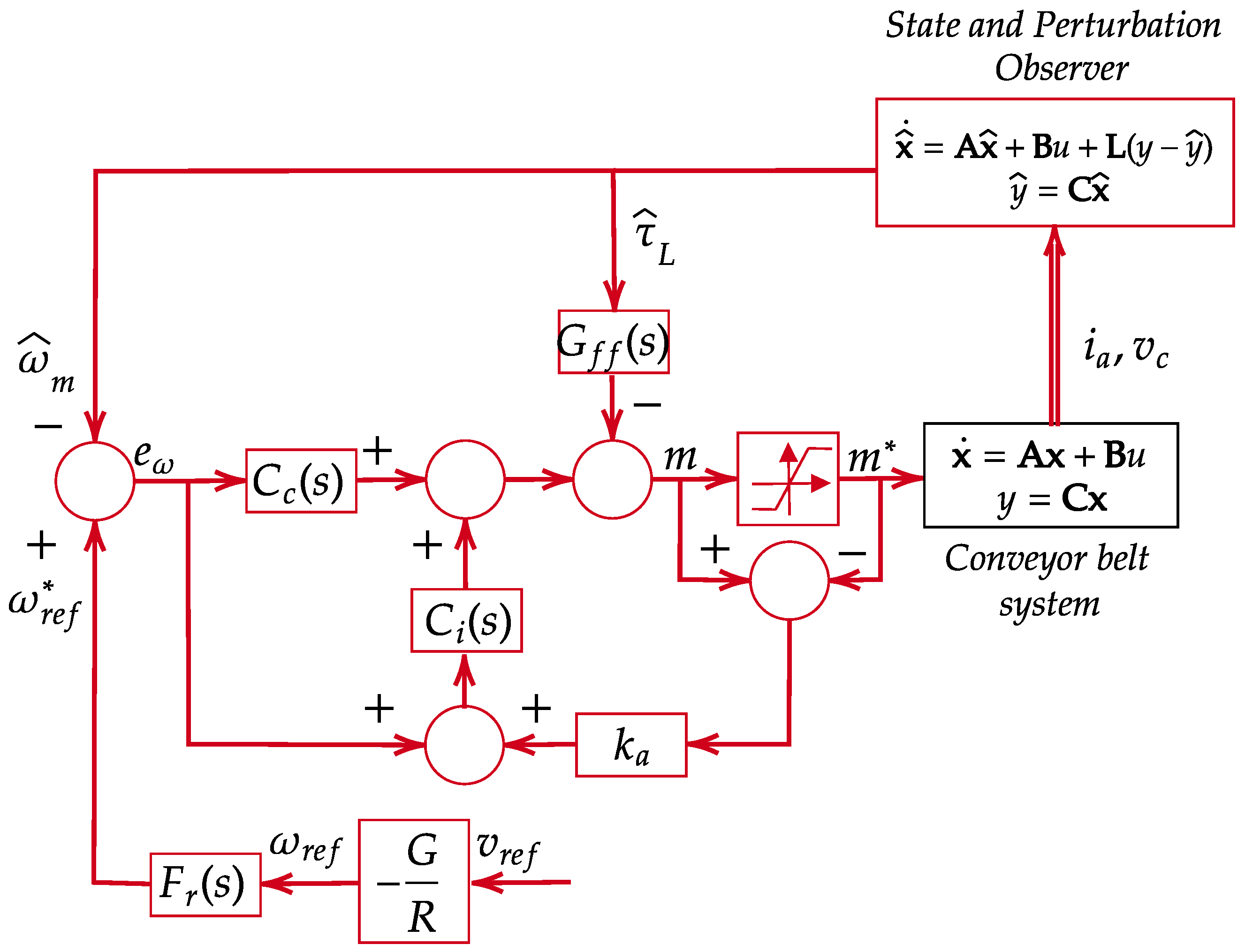
4.5. Proposed Control Scheme

Figure 20 illustrates the complete control scheme proposed to regulate the angular velocity of the rotor’s motor, ensuring a uniform linear velocity in the movement of the conveyor belt.

This control scheme demonstrates how the previously sized components are incorporated. Additionally, three extra elements are included within the overall scheme. First, a gain is introduced to convert the desired reference linear velocity of the conveyor belt to the corresponding angular velocity of the motor. The second block is a low-pass filter, designed to mitigate sudden changes in the reference applied as the control loop’s input. The transfer function of this reference filter is given by

$$F_r\left(s\right)={\displaystyle \frac{1}{0.4s+1}}$$

(35)

The cutoff frequency of the reference filter ($F_r\left(s\right)$) was chosen to ensure that the Nyquist plot of the transfer function does not transition from positive to negative real values, as illustrated in Figure 11. Additionally, an anti-windup scheme was incorporated to mitigate the adverse effects caused by the saturation of the modulating signal within the range $(-1,1)$.

The development of the anti-windup scheme involves deriving an expression for the proposed velocity controller, where each contributing action is explicitly identified. This allows the controller to be decomposed as follows: $C\left(s\right)=C_c\left(s\right)+C_i\left(s\right)$, where $C_c\left(s\right)$ represents the effects produced by the lead compensator and the proportional actions, and $C_i\left(s\right)$ denotes the integral action.

This structure is essential for implementing the anti-windup scheme, enabling the integral action to be nullified when the modulating signal becomes saturated. Thus, it is obtained that $C_c\left(s\right)=0.03{\displaystyle \frac{0.083s+1}{0.003s+1}}$, and $C_i\left(s\right)={\displaystyle \frac{0.05}{s}}$. The $k_a$ gain associated with the anti-windup strategy is established as $k_a=20$.

5. Discussion

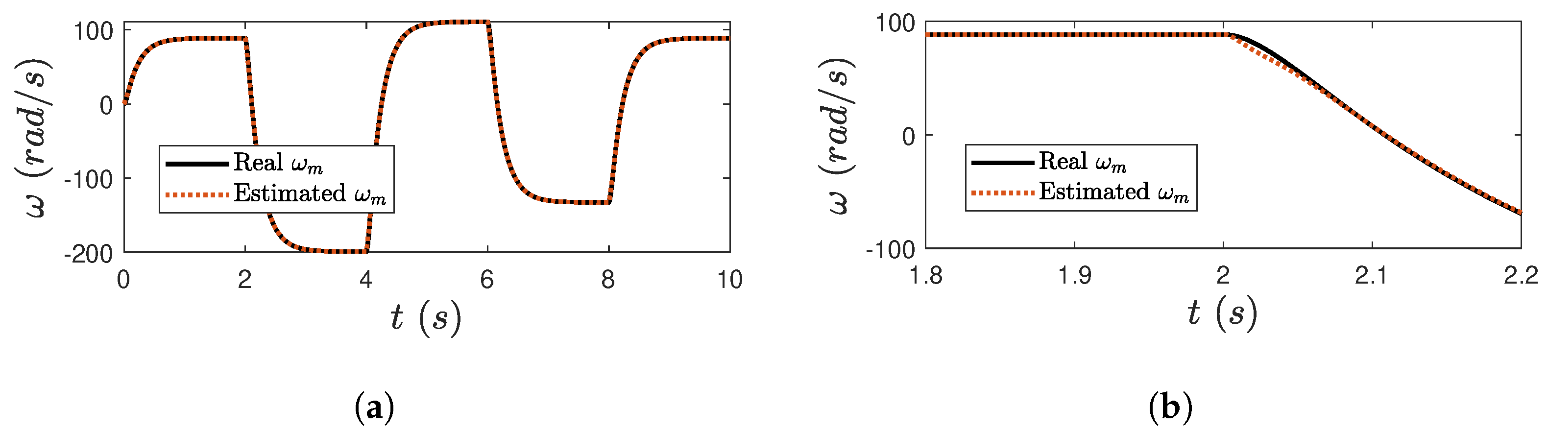
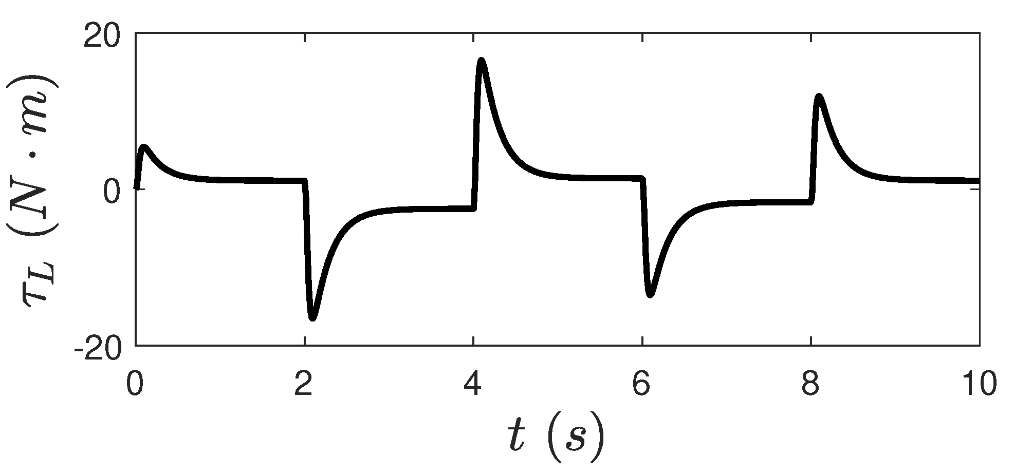
5.1. Performance Evaluation of the Proposed Observer

The proposed observer must be evaluated based on its ability to estimate the state variables that describe the dynamics of the DC motor and the load torque applied to its rotor. Additionally, its performance must be tested under conditions of parameter uncertainties and measurement noise in the electrical signals used for the estimation process.

This evaluation will be divided into two parts: In the first part, the observer will be assumed to have ideal parameters, perfectly matching the real values of the DC motor, and the measurements of $i_a$ and $v_a$ will be considered as noise free. In the second part, the assessment will consider the presence of parameter uncertainties in the model underlying the observer, along with low-magnitude, high-frequency measurement noise affecting both electrical variables during the observation process.

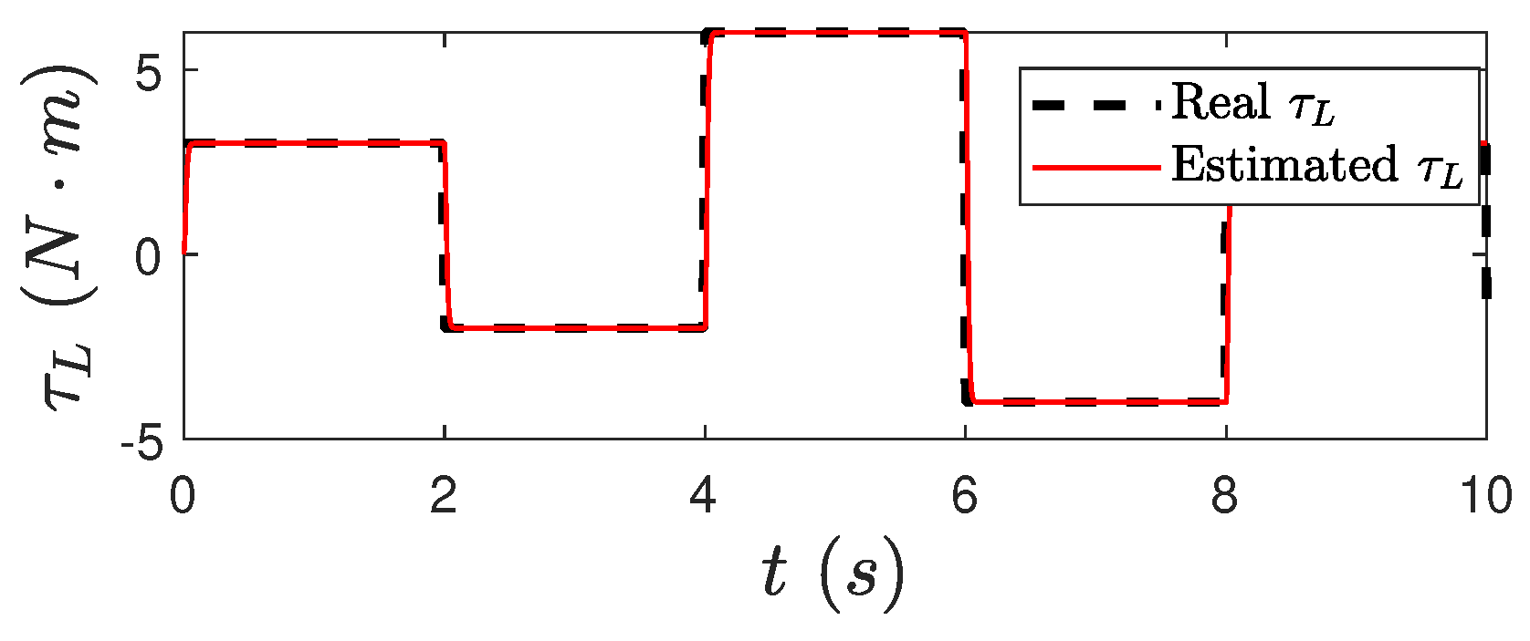
5.1.1. Test 1: Estimation Process Under Ideal Conditions

This test is conducted by applying the modulating signals shown in Figure 8a, under open-loop operational conditions for the entire system. The variables analyzed include the armature current, which serves as the state variable for the estimation process; the angular velocity, which accurate estimation validates the proper functioning of the observer; and the load torque, a critical parameter for implementing feedforward-based compensation. This test assumes that the DC motor is initially at rest and begins operating at the start of the test.

Figure 21 illustrates how the observer accurately replicates the armature current as an internal state, demonstrating its ability to converge its internal state variables to the actual system states. This is achieved despite the observer having a lower order compared to that of the real system.

Figure 22 illustrates the estimation process for the rotor’s angular velocity. The observer accurately estimates both the armature current and rotor’s angular velocity with minimal delay, making it highly suitable for implementing a sensorless control scheme to regulate the velocity, as shown in Figure 20.

Notably, a small error occurs when the angular velocity changes abruptly. This behavior is attributed to the bandwidth configuration of the implemented observer. When the rate of change in the angular velocity exceeds the bandwidth of this observer, such estimation errors are expected. However, this issue can be mitigated when the control scheme is applied, as it restricts the frequency range within which the angular velocity operates.

Figure 23 illustrates the estimation process for the load torque. By analyzing the differential equation governing the mechanical subsystem of the DC motor, as presented in Equation (8), it can be demonstrated that this mechanical variable remains constant under steady-state operating conditions, as depicted in the figure. However, during testing, the estimated load torque showed variations when the operating point of the observed system was altered, primarily because of changes in the modulating signals. In this situation, ${\displaystyle \frac{d}{dt}}{\tau }_L\ne 0$. Despite this, the structure of the proposed observer proves to be effective under ideal operating conditions, as its internal states exhibit rapid convergence to the actual states of the DC motor.

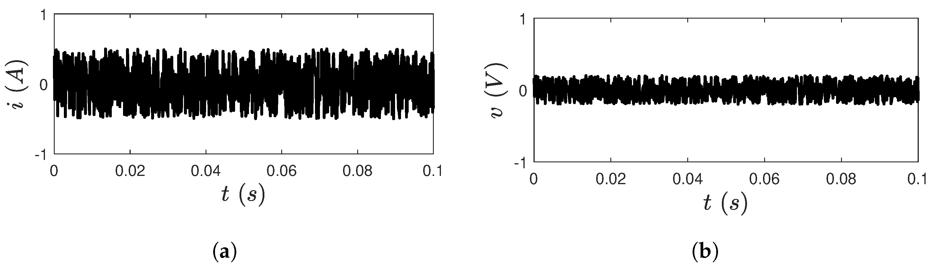
5.1.2. Test 2: Estimation Process Considering Parameter Uncertainties and Measurement Noises

In the previous test, it was demonstrated that the proposed state observer performs effectively under ideal operating conditions, assuming the absence of measurement noise and parameter uncertainties. In this test, the robustness of this component within the control scheme will be analyzed.

Table 4. Parameter uncertainties of the state observer.

Parameter	Unit	Value	Percentage
J	$\mathrm{kg}·{\mathrm{m}}^2$	6.54 × 10−3	−6%
b	${\displaystyle \frac{\mathrm{N}·\mathrm{m}·\mathrm{s}}{\mathrm{rad}}}$	1.76 × 10−3	+2%
$V_n$	V	90	-
$k_i$	${\displaystyle \frac{\mathrm{N}·\mathrm{m}}{\mathrm{A}}}$	0.320	−8%
$k_{\omega }$	${\displaystyle \frac{\mathrm{V}·\mathrm{s}}{\mathrm{rad}}}$	0.368	+5%
$L_a$	mH	31.28	+10%
$R_a$	$\Omega$	1.33	+5%

presents the uncertainties introduced to the state observer, expressed as percentage deviations from the actual parameters of the DC motor.

Figure 24 presents the measurement noise injected into the state observer. These noises are introduced through the measurement of electrical variables used to estimate the mechanical variables of interest. The noise signals are characterized by a low magnitude and a high frequency. Such signals are generated as random signals with a specified amplitude and a maximum frequency of 200 rad/s. The maximum magnitude of current noises is 0.5 A; meanwhile, the noises associated with the voltage measurements have a maximum amplitude of 0.2 V. These noise signals will be applied to the measurements throughout the entire test. These measurement noises can be generated by electromagnetic interferences and mechanical vibrations of these sensors, which are typically high-frequency signals.

Figure 25 shows the measurements of the electrical variables used by the state observer. Additionally, Figure 25c,d presents the estimation of the armature current, allowing a comparison with the noisy measurements used for the estimation. It is noteworthy that although the noisy signal is considered as the actual state variable, the estimated value converges to the true state because of the bandwidth of the proposed state observer, which effectively rejects high-frequency noises. The observer’s gains play a crucial role in this process: Higher gains result in faster observer dynamics but also increase its sensitivity to noise. This test demonstrates the ability of the observer to accurately estimate state variables despite the presence of high-frequency noise in the measurements.

To evaluate the performance of the state observer, an IAE-based criterion index is employed. The reference signal is the actual armature current, and the errors are calculated as the difference between the estimated and measured values. The IAE value for the measured armature current is 1.3573, while that for the estimated signal is significantly lower at 0.2205. A lower IAE value, closer to zero, indicates a lower total error between the processed signals. This demonstrates the effectiveness of the state observer in attenuating high-frequency noise present in the measured state variables.

Figure 26 illustrates the performance of the observer in estimating the mechanical variables required for implementing the sensorless control scheme. For the rotor’s angular velocity, the results demonstrate that even without direct measurements of this variable, the observer accurately approximates the actual rotational speed of the rotor’s motor. A minor deviation is observed, with a mean absolute error of 6.86 rad/s throughout the test. This deviation may be attributed to parameter uncertainties in the values used to characterize the DC motor.

The estimated load torque is also presented, displaying behavior similar to that observed in Figure 23, where the performance of the state observer was analyzed under ideal conditions. The mean absolute error between the estimated (Figure 26c) and actual load torques (Figure 23) is 0.3891 N·m. This difference is primarily because of the high-frequency components present in the estimated load torque during this test. It is important to note, as shown in Figure 19, that such high-frequency noise will be attenuated by the combined effects of the inherent sensitivity of the proposed feedback-based control scheme and the feedforward regulator. Consequently, this discrepancy is expected to be even smaller when the DC motor is under control.

5.2. Sensorless Control Scheme’s Evaluation

Thus, the tests conducted in the previous section demonstrate the capability of the proposed observer to estimate the mechanical variables that characterize the mechanical subsystem of the analyzed DC motor. These results provide a solid foundation for implementing the sensorless control scheme under the conditions to which the observer was subjected.

In this section, two additional tests will be performed. The first test assesses the ability of the controlled scheme to handle changes in the velocity reference established for the conveyor belt’s movement. The second test evaluates the performance of the scheme when subjected to variations in the mass transported on the conveyor while maintaining a constant velocity reference.

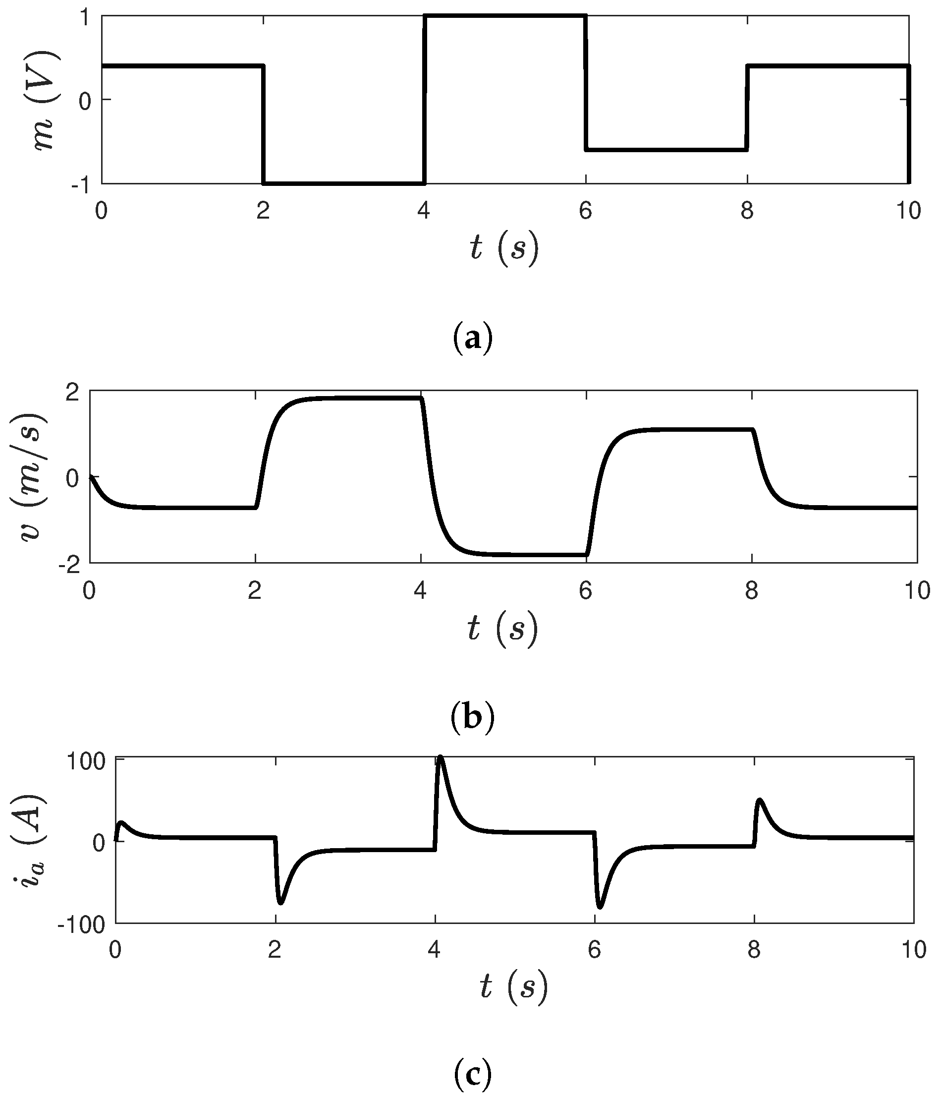
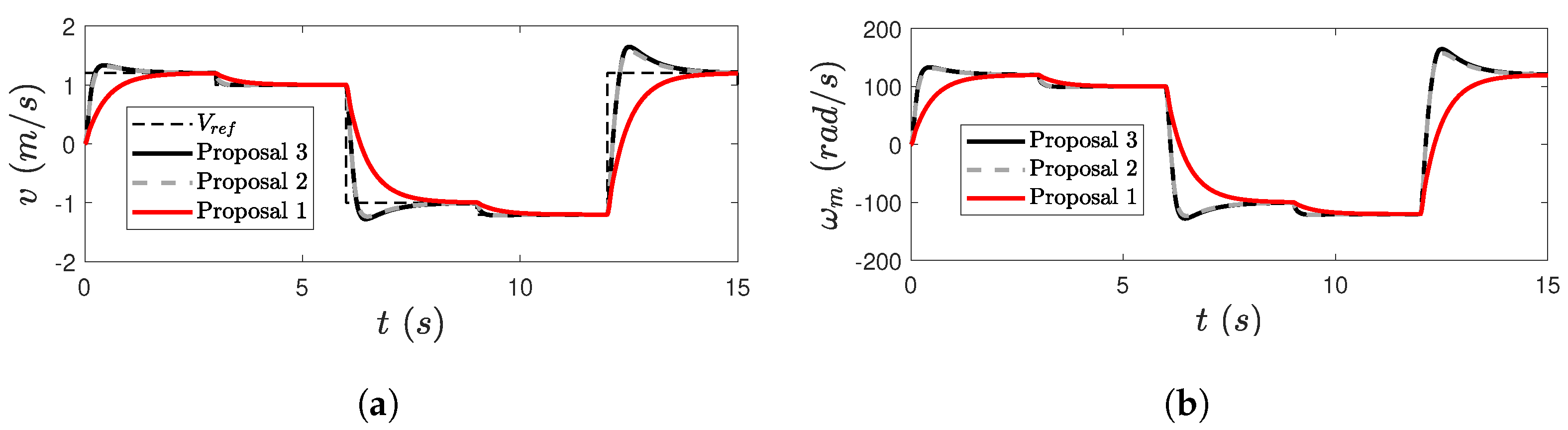
5.2.1. Test 1: Changes in the Velocity Reference’s Value

In this test, a comparison will be made between various control schemes derived from the proposed approach. The simplest scheme employs only the angular-velocity controller, as initially proposed, relying directly on measurements of this variable to close the control loop. This control scheme will be defined as Proposal 2. Another scheme, although still utilizing these measurements, incorporates both a feedforward strategy and a state observer to enhance the performance. Such a control scheme will be defined as Proposal 3. In both of these previous proposals, which will be compared with the scheme shown in Figure 20, the reference prefiltering stage is not included. These previous control schemes are presented in Figure 27.

Figure 28 shows the behaviors of both the linear velocity of the conveyor belt and the angular velocity of the rotor when the tested control schemes are applied. These schemes are evaluated based on their ability to regulate the behavior of the conveyor belt in response to the reference input provided to the control system. The state observer is assumed to operate under ideal conditions. The references applied in this test are presented in Figure 28a.

Figure 28a illustrates that all the proposed control schemes successfully follow the reference throughout the entire test. Notably, in schemes where the prefiltering stage is not applied, the response is faster; however, an overshoot occurs whenever there is a change in the applied reference. In

Table 5. Assessment of the controller’s performance based on index criteria.

Parameter	IAE	ISE
Proposed Scheme 1	0.1927	0.1814
Proposed Scheme 2	0.0888	0.0694
Proposed Scheme 3	0.0942	0.0719

, the performance of each control scheme used to obtain the results shown in Figure 28 is quantified using time-normalized indices based on the IAE and ISE criteria.

The control schemes that do not incorporate prefiltering demonstrate their ability to track changes in the velocity reference, as their index-based criteria are relatively close to zero compared to those of the proposed scheme, which includes prefiltering. Therefore, when evaluating the performance of control schemes in tracking velocity references, the absence of a prefiltering stage reduces the effectiveness of the control scheme under such operating conditions.

A similar behavior to that observed in the conveyor belt’s velocity is also noted in the angular velocity of the DC motor’s rotor. A key advantage of the proposed control scheme, which incorporates a prefiltering stage, is the smoothness of the resulting signals in both velocity profiles. Figure 29 illustrates the performances of the armature current and the estimated load torque.

As observed in the previous results, the armature current exhibits a noticeable overshoot in response to reference changes when the prefiltering stage is not applied. This overshoot is detrimental to the DC motor, potentially compromising the integrity of the equipment. The prefiltering stage mitigates this issue by reducing the bandwidth of the entire control scheme, resulting in smoother behavior at the expense of a slower reaction speed in the loop. Therefore, the prefiltering stage is essential to ensure the safe operation of the controlled DC motor. This result can be reinforced by the data presented in

Table 6. Armature current overshoots presented along the entire test.

Control Scheme	Reference 1	Reference 2	Reference 3	Reference 4	Reference 5
Proposed Scheme 1	−22.84 A	-	33.51 A	-	−40.31 A
Proposed Scheme 2	−59.55 A	24.61 A	82.02 A	20.78 A	−86.52 A
Proposed Scheme 3	−59.55 A	24.61 A	82.02 A	20.78 A	−86.52 A

, presenting the armature current overshoots observed when the controlled systems are subjected to reference changes.

The data presented in Figure 29a and Table 6 highlight the importance of the prefiltering stage in preventing peak currents, which can pose a significant risk to the integrity of the DC motor. Although this element results in reduced performance when tracking velocity references, it ensures a safer operation of the actuator during changes in the conveyor belt’s velocity.

Figure 29b presents the estimation of the load torque, where the control scheme constituting Proposal 2 does not incorporate the use of a state observer, resulting in ${\tau }_L=0$ throughout the entire test. As the bandwidth of the control scheme increases, the load torque during transients also rises, indicating greater effort required from the DC motor. Figure 30 illustrates the performance of the modulating signal applied to the power converter.

The performance of the control scheme can be evaluated by analyzing the behavior of the modulating signals it generates. When the prefiltering stage is applied, the modulating signal remains smooth and avoids reaching maximum or minimum values during transients. This behavior contrasts with the case where the prefiltering stage is not included, as high peaks are observed under similar operational conditions. When these peaks occur, the anti-windup scheme effectively prevents oversaturation by mitigating the impact of invalid values of m. In

Table 7. Quantification of changes in modulating signals generated by the control schemes used in the test.

Parameter	IAE
Proposed Scheme 1	0.3573
Proposed Scheme 2	0.7162
Proposed Scheme 3	0.7054

, the changes in the modulating signals generated by each control scheme used for developing this test are quantified by considering a time-normalized IAE-based criterion.

As previously discussed, the quantification revealed that the inclusion of the prefiltering stage significantly reduces changes in the modulating signals, resulting in smoother transitions and effectively preventing the armature current overshoots analyzed earlier.

These results clearly highlight the importance of incorporating a prefiltering stage to mitigate potential armature current overshoots and peaks in the modulating signals. However, a drawback of including this element is the reduced performance of the closed-loop control system during reference input changes.

One effective approach is to introduce a unity-gain low-pass filter with a cutoff frequency set one decade lower than the frequency at which the Nyquist plot of the open-loop transfer function (${\displaystyle \frac{{\omega }_m\left(s\right)}{m\left(s\right)}}$) transitions from positive to negative real values. In this case, the controller within the angular-velocity regulation’s feedback loop will be confined to a specific frequency range below the cutoff frequency of the filter.

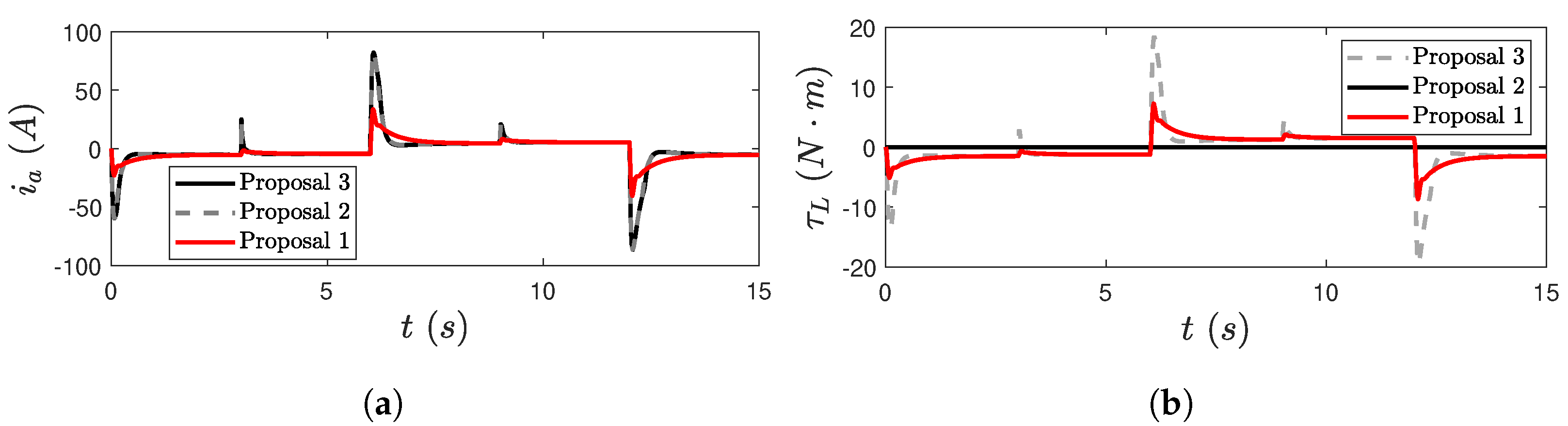
5.2.2. Test 2: Abrupt Changes in the Torque Load at a Constant Velocity Reference Value

In the previous test, the effectiveness of the feedforward component integrated into the proposed control scheme was not clearly demonstrated, as the mass on the conveyor belt was assumed to remain constant throughout the test. To fully analyze the impact of this component, the following test is conducted, where the load torque is abruptly changed at a specific time. This consideration is introduced to evaluate the feedforward element under operational conditions where the external disturbance consists of a broad range of frequency components. Figure 31 presents the load torque applied to the motor’s rotor, alongside the load torque estimated by the proposed observer.

The results displayed in the previous figure demonstrate that the state observer estimates the load torque quickly and accurately. Leveraging the capabilities of the proposed observer, the feedforward scheme can be implemented using its torque estimation under ideal conditions. Figure 32 illustrates the behavior of the controlled system, specifically, the angular velocity of the motor’s rotor. This control scheme incorporates the sensorless version of the control configuration depicted in Figure 20.

This test demonstrates the advantages of applying a feedforward compensation scheme to manage the negative effects, produced by abrupt external perturbations, on the controlled dynamic system. Including this type of compensator enhances the ability of the control loop to maintain the angular velocity’s stability despite external disturbances, such as variations in the load torque applied to the motor’s rotor. These perturbations are nearly instantaneously rejected.

Table 8. Quantification of the impact of the feedforward compensator on the proposed control scheme.

Parameter	IAE	ISE
With Compensator	0.0533	2.9153
Without Compensator	0.0688	3.1454

presents the index-based criteria used to quantify the performance improvement of the controlled DC motor when the feedforward compensator is applied. These criteria are time- and magnitude-normalized, taking into account the amount of processed data and the reference’s angular velocity.

The numerical values of these index criteria highlight the significant performance enhancement achieved by implementing the proposed feedforward compensation method in the controlled actuator.

Figure 33 compares the behaviors of the armature current with and without the proposed compensator. Despite the significant improvement in the angular velocity observed throughout the test, there is no noticeable variation in the performance of this state variable. This result highlights the importance of the compensator in safely managing abrupt external perturbations. This compensator may be less effective in applications where the external perturbation lacks wide-frequency-range components, particularly when such perturbations are characterized by low-frequency components.

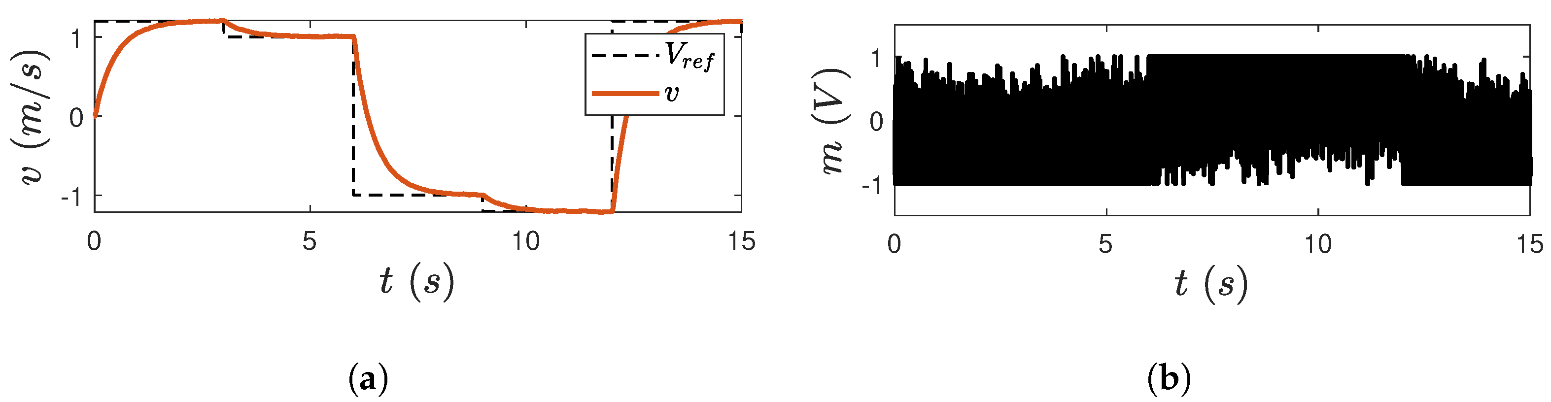
5.2.3. Test 3: Non-Ideal Operational Conditions

This test analyzes the performance of the proposed control scheme when the state observer operates under non-ideal conditions, such as measurement noise and parameter uncertainties in its internal configuration. The measurement noise considered in this test is shown in Figure 24, while the parameter uncertainties are presented in Table 4. Figure 34 illustrates the performance of the entire sensorless control scheme in the presence of measurement noise.

The proposed control scheme is capable of regulating the entire system, despite the presence of measurement noise. However, these noises negatively impact the modulating signals generated by the control scheme. Therefore, measures must be implemented to mitigate this undesirable behavior, as it can affect the integrity of the actuator, including the internal switches of the power converter, and lead to increased power losses because of high-frequency switching.

Figure 35 shows the behavior of the entire system when both measurement noise and parameter uncertainties are present within the state observer. The results from this test demonstrate that the sensorless control scheme loses some of its regulation capability because of the parameter uncertainties introduced to the state observer. Despite these operational challenges, the control scheme is still able to regulate the system but not with a high degree of precision, leading to variations that could negatively impact the integrity of the DC motor.

The undesirable behavior presented in Figure 35 can be mitigated using angular-velocity sensors to eliminate the effects of parameter uncertainties. This solution means an increase in the cost of the proposed control scheme. If developing a sensorless control scheme is preferred, a parameter identification technique can be implemented to enhance the robustness of the sensorless approach.

From the results presented above, it is possible to compare the specific contributions of this work with those reported in the state of the art.

Table 9. Comparison among different control schemes used for regulating DC motors.

Work	Motor	Control Scheme	Performance
[12]	A multi-input, multi-output, separately excited DC motor	It combines the advantages of adaptive backstepping and integral sliding mode control (ISMC) to improve the overall robustness of the system.	IAE = 3.086 ISE = 41.36 $t_s$ = 0.477 s
[29]	Full-bridge buck inverter–DC motor	The control system performs trajectory tracking of the angular velocity of the DC motor shaft without relying on electromechanical sensors.	Qualitative results for the capability of the control scheme to track Bezier-based velocity trajectories
[30]	Permanent magnet DC motor	Sliding mode control method based on a washout filter (SMC-w) for speed control.	$t_s=0.02$ s − 0.076 s Output speed overshoot: 0.33% Steady-state error ≈ 0.1
This work	Full H-bridge power converter used for regulating a permanent magnet DC motor	Based on a PI controller combined with a lead compensator and an external perturbation compensator consisting of a feedforward mechanism with a low-order filter and a state and perturbation observer.	Without changes in the speed reference and abrupt changes in the external perturbation: IAE = 0.0533 and ITE = 2.9153 With changes in the speed reference: IAE = 0.1927 and ITE = 0.1814

shows the advantages of this controller against other conventional ones, where the robustness of the response in the speed control of the DC motor stands out.

6. Conclusions

This research developed a dynamic model of a system comprising a full H-bridge power converter, a permanent magnet DC motor, and a conveyor belt. The models were formulated using state-space representations and transfer functions. A frequency-domain analysis of the DC motor was conducted, considering two transfer functions to evaluate the effects of input voltages and external perturbations. The analysis included examining their magnitudes and phase responses, as well as their Nyquist plots.

Following the modeling process, a control scheme was developed comprising a PI controller with a lead compensator, an external disturbance rejection scheme featuring a state observer, and a feedforward compensator integrated with a low-pass filter. The tuning procedure for each component was presented, including a frequency-response-based analysis to obtain a compact and well-justified control scheme. The PI controller, coupled with the lead compensator, was designed to ensure a bandwidth of 30.5 rad/s, a gain margin of 101°, and a phase margin of 20.7 dB.

The feedforward compensator was developed based on the sensitivity transfer function, which was used to analyze the disturbance rejection capability of the DC motor against load torque variations. Using this transfer function, a low-pass filter was proposed, with a gain of −14.9 dB and a bandwidth of 31.7 rad/s, selected to align with the disturbance rejection capability of the DC motor.

The state observer was designed to estimate the load torque applied to the motor’s rotor. To simplify the observer, the load torque was modeled as a constant term, reducing its order. The bandwidth of the load torque observer was selected to ensure that the estimation process does not negatively impact the regulator’s operation. A bandwidth of 160 rad/s was chosen, with observer gains set at levels that prevent the excessive amplification of the measurement noise.

Several tests were conducted to evaluate the effectiveness of the proposed control scheme under various operational conditions, highlighting the performance of each internal component. The state observer was tested in multiple scenarios.

In the first test, ideal operating conditions were considered to assess the observer’s performance. It was demonstrated that all the states were estimated almost instantaneously. Subsequently, the state observer was tested under more challenging conditions, including the presence of measurement noise and parameter uncertainties. The estimation process was evaluated using the IAE index, showing that the estimated state variables were more accurate than the measured ones. Specifically, the error associated with the armature current was reduced from 1.353 to 0.2205.

A minor deviation was observed, with a mean absolute error of 6.86 rad/s throughout the test. This deviation is likely attributed to parameter uncertainties in the values used to characterize the DC motor. Additionally, the mean absolute error between the estimated load torque and the actual load torque was 0.3891 N·m. This discrepancy is primarily because of the presence of high-frequency components in the estimated load torque during the test.

After demonstrating the performance of the observer state, the sensorless control scheme was assessed using IAE- and ISE-based indices and analysis related to overshot armature currents. It was demonstrated that the use of a prefiltering stage is crucial to avoid the presence of high overshoot currents without compromising the accuracy of the control scheme proposed. Using such a scheme, considering velocity reference variations, those peaks were reduced around 50%, and the IAE and ISE indices were both lower than 0.2 units. These results were supported by the variation that the modulation signals had, which had an IAE index of 0.353, which is much lower than the cases when a prefiltering stage was not considered.

The feedforward and load torque estimator was demonstrated to be very effective when the load torque changed abruptly, producing lower values of IAE and ISE indices, which were 0.0533 and 2.915 units, respectively. Lastly, the disadvantage of the sensorless control scheme was highlighted, as it is highly sensitive to parameter uncertainties, which can affect its performance. Such decreases in the performance of the controlled system were demonstrated by the high error rate in the stationary state and the high-frequency oscillations shown in the velocity to be controlled.

The results of this research can be further enhanced through experimental testing. These improvements can be achieved by implementing the proposed control scheme in a physical system, allowing for a comprehensive validation of its performance. As future work, integrating the system into an industrial environment for a specific conveyor process is recommended.

References

1. Sankardoss, V.; Geethanjali, P. PMDC Motor Parameter Estimation Using Bio-Inspired Optimization Algorithms. IEEE Access 2017, 5, 11244–11254. [Google Scholar] [CrossRef]
2. Barkas, D.A.; Ioannidis, G.C.; Psomopoulos, C.S.; Kaminaris, S.D.; Vokas, G.A. Brushed DC Motor Drives for Industrial and Automobile Applications with Emphasis on Control Techniques: A Comprehensive Review. Electronics 2020, 9, 887. [Google Scholar] [CrossRef]
3. Coral-Enriquez, H.; Pulido-Guerrero, S.; Cortés-Romero, J. Robust disturbance rejection based control with extended-state resonant observer for sway reduction in uncertain tower-cranes. Int. J. Autom. Comput. 2019, 16, 812–827. [Google Scholar] [CrossRef]
4. Baidya, D.; Dhopte, S.; Bhattacharjee, M. Sensing System Assisted Novel PID Controller for Efficient Speed Control of DC Motors in Electric Vehicles. IEEE Sens. Lett. 2023, 7, 6000604. [Google Scholar] [CrossRef]
5. Silva-Ortigoza, R.; Hernández-Márquez, E.; Roldán-Caballero, A.; Tavera-Mosqueda, S.; Marciano-Melchor, M.; García-Sánchez, J.R.; Hernández-Guzmán, V.M.; Silva-Ortigoza, G. Sensorless Tracking Control for a “Full-Bridge Buck Inverter–DC Motor” System: Passivity and Flatness-Based Design. IEEE Access 2021, 9, 132191–132204. [Google Scholar] [CrossRef]
6. García-Chávez, R.E.; Silva-Ortigoza, R.; Hernández-guzmáN, V.M.; Marciano-Melchor, M.; Orta-Quintana, A.A.; García-Sánchez, J.R.; Taud, H. A Robust Sliding Mode and PI-Based Tracking Control for the MIMO “DC/DC Buck Converter–Inverter–DC Motor” System. IEEE Access 2023, 11, 119396–119408. [Google Scholar] [CrossRef]
7. Ismail, A.A.A.; Elnady, A. Advanced Drive System for DC Motor Using Multilevel DC/DC Buck Converter Circuit. IEEE Access 2019, 7, 54167–54178. [Google Scholar] [CrossRef]
8. Chen, J.; Maksimovic, D.; Erickson, R. Buck-boost PWM converters having two independently controlled switches. In Proceedings of the 2001 IEEE 32nd Annual Power Electronics Specialists Conference (IEEE Cat. No.01CH37230), Vancouver, BC, Canada, 17–21 June 2001; Volume 2, pp. 736–741. [Google Scholar] [CrossRef]
9. Ardhenta, L.; Subroto, R.K. Feedback Control for Buck Converter—DC Motor Using Observer. In Proceedings of the 2020 12th International Conference on Electrical Engineering (ICEENG), Cairo, Egypt, 7–9 July 2020; pp. 30–33. [Google Scholar] [CrossRef]
10. Liceaga-Castro, J.U.; Siller-Alcalá, I.I.; González-San Román, J.D.; Alcántara-Ramírez, R.A. PI Speed Control with Reverse Motion of a Series DC Motor Based on the Noise Reduction Disturbance Observer. Actuators 2022, 11, 117. [Google Scholar] [CrossRef]
11. Rahmatullah, R.; Ak, A.; Serteller, N.F.O. SMC Controller Design for DC Motor Speed Control Applications and Performance Comparison with FLC, PID and PI Controllers. In Intelligent Sustainable Systems; Nagar, A.K., Singh Jat, D., Mishra, D.K., Joshi, A., Eds.; Springer: Singapore, 2023; pp. 607–617. [Google Scholar]
12. Afifa, R.; Ali, S.; Pervaiz, M.; Iqbal, J. Adaptive Backstepping Integral Sliding Mode Control of a MIMO Separately Excited DC Motor. Robotics 2023, 12, 105. [Google Scholar] [CrossRef]
13. Vesović, M.; Jovanović, R.; Trišović, N. Control of a DC motor using feedback linearization and gray wolf optimization algorithm. Adv. Mech. Eng. 2022, 14, 16878132221085324. [Google Scholar] [CrossRef]
14. Khasawneh, H.J.; Abdelaal, O.; Saaideh, M.I.A.; Abo-Hammour, Z.S. Optimal Lead Compensator for Two-Loop Control System of Linear DC Motor. In Proceedings of the 2019 IEEE Jordan International Joint Conference on Electrical Engineering and Information Technology (JEEIT), Amman, Jordan, 9–11 April 2019; pp. 634–639. [Google Scholar] [CrossRef]
15. Slough, J.; Belcher, M.; Tsui, T.; Bhattacharya, S. Modeling and Simulation of Electric Vehicles Using Simulink and Simscape. In Proceedings of the 2021 IEEE 94th Vehicular Technology Conference (VTC2021-Fall), Norman, OK, USA, 27–30 September 2021; pp. 1–6. [Google Scholar] [CrossRef]
16. Yazdani, A.; Iravani, R. Voltage-Sourced Converters in Power Systems: Modeling, Control, and Applications; John Wiley & Sons: Hoboken, NJ, USA, 2010. [Google Scholar]
17. Vasca, F.; Iannelli, L. Dynamics and Control of Switched Electronic Systems: Advanced Perspectives for Modeling, Simulation and Control of Power Converters; Springer: Berlin/Heidelberg, Germany, 2012. [Google Scholar]
18. Katsioula, A.G.; Karnavas, Y.L.; Boutalis, Y.S. An enhanced simulation model for DC motor belt drive conveyor system control. In Proceedings of the 2018 7th International Conference on Modern Circuits and Systems Technologies (MOCAST), Thessaloniki, Greece, 7–9 May 2018; pp. 1–4. [Google Scholar] [CrossRef]
19. Hace, A.; Jezernik, K.; Sabanovic, A. SMC With Disturbance Observer for a Linear Belt Drive. IEEE Trans. Ind. Electron. 2007, 54, 3402–3412. [Google Scholar] [CrossRef]
20. Sabanovic, A.; Sozbilir, O.; Goktug, G.; Sabanovic, N. Sliding mode control of timing-belt servosystem. In Proceedings of the 2003 IEEE International Symposium on Industrial Electronics (Cat. No.03TH8692), Rio de Janeiro, Brazil, 9–11 June 2003; Volume 2, pp. 684–689. [Google Scholar] [CrossRef]
21. Garelli, F.; Mercedes Ramírez, M.; Ariel Domínguez, C.; Modesto Angulo, A. Simulación de un algoritmo para controlar el nivel en tolva ante alimentación discontinua de caña. Rev. Iberoam. Automática Informática Ind. RIAI 2009, 6, 54–60. [Google Scholar] [CrossRef]
22. Mahmoud, M. Robust Control and Filtering for Time-Delay Systems, 1st ed.; CRC Press: Boca Raton, FL, USA, 2000. [Google Scholar] [CrossRef]
23. Antritter, F.; Maurer, P.; Reger, J. Flatness based control of a buck-converter driven DC motor. IFAC Proc. Vol. 2006, 39, 36–41. [Google Scholar] [CrossRef]
24. Domański, P.D. Index Ratio Diagram—A New Way to Assess Control Performance. In Proceedings of the 2024 European Control Conference (ECC), Stockholm, Sweden, 25–28 June 2024; pp. 2041–2046. [Google Scholar] [CrossRef]
25. Dogruer, T.; Can, M.S. Design and robustness analysis of fuzzy PID controller for automatic voltage regulator system using genetic algorithm. Trans. Inst. Meas. Control 2022, 44, 1862–1873. [Google Scholar] [CrossRef]
26. Gurugubelli, V.; Ghosh, A.; Panda, A.K. Droop controlled voltage source converter with different classical controllers in voltage control loop. In Proceedings of the 2022 IEEE International Conference on Power Electronics, Smart Grid, and Renewable Energy (PESGRE), Trivandrum, India, 2–5 January 2022; pp. 1–6. [Google Scholar] [CrossRef]
27. Wang, J.; Wu, G.; Sun, B.; Ma, F.; Aksun-Guvenc, B.; Guvenc, L. Disturbance Observer-Smith Predictor Compensation-Based Platoon Control with Estimation Deviation. J. Adv. Transp. 2022, 2022, 9866794. [Google Scholar] [CrossRef]
28. Yue, L.; Wang, Y.; Xiao, B.; Wang, Y.; Lin, J. Improved active disturbance rejection speed control for autonomous driving of high-speed train based on feedforward compensation. Sci. Prog. 2023, 106, 00368504231208505. [Google Scholar] [CrossRef] [PubMed]
29. Orta-Quintana, Á.A.; García-Chávez, R.E.; Silva-Ortigoza, R.; Marciano-Melchor, M.; Villarreal-Cervantes, M.G.; García-Sánchez, J.R.; García-Cortés, R.; Silva-Ortigoza, G. Sensorless Tracking Control Based on Sliding Mode for the “Full-Bridge Buck Inverter–DC Motor” System Fed by PV Panel. Sustainability 2023, 15, 9858. [Google Scholar] [CrossRef]
30. Velasco-Muñoz, H.; Candelo-Becerra, J.E.; Hoyos, F.E.; Rincón, A. Speed Regulation of a Permanent Magnet DC Motor with Sliding Mode Control Based on Washout Filter. Symmetry 2022, 14, 728. [Google Scholar] [CrossRef]
Figure 1. Equivalent circuit of a full H-bridge.
Eng 06 00042 g001
Figure 2. Combinations used for manipulating the output voltage of the full H-bridge.
Eng 06 00042 g002
Figure 3. Equivalent circuit of a permanent magnet DC motor.
Eng 06 00042 g003
Figure 4. Block diagram used for representing the DC motor according to the previous transfer functions.
Eng 06 00042 g004
Figure 5. Representation of a generic conveyor belt.
Eng 06 00042 g005
Figure 6. Dynamic characteristics of the conveyor’s actuator in the frequency domain. (a) Bode diagram of G 1 ( s ) ; (b) Bode diagram of G 2 ( s ) ; (c) Nyquist plot of G 1 ( s ) ; (d) Nyquist plot of G 2 ( s ) .
Eng 06 00042 g006
Figure 7. Analysis of the root loci associated with the transfer functions G 1 ( s ) and G 2 ( s ) . (a) Root locus associated with G 1 ( s ) . (b) Root locus associated with G 2 ( s ) . (c) Zoomed-in view of the root locus corresponding to G 1 ( s ) . (d) Zoomed-in view of the root locus corresponding to G 2 ( s ) . The trajectories are presented with different colors for better understanding.
Eng 06 00042 g007
Figure 8. Performance of the conveyor belt under modulating signals in an open-loop configuration: (a) PWM-modulating reference signal. (b) Velocity at which the conveyor transports the sugarcane. (c) Armature current that is conducted through the DC motor.
Eng 06 00042 g008
Figure 9. Frequency domain assessment of applying the PI controller to regulate the angular velocity of the DC motor.
Eng 06 00042 g009
Figure 10. Frequency domain assessment of applying the PI + a lead compensator controller to regulate the angular velocity of the DC motor.
Eng 06 00042 g010
Figure 11. Nyquist plot corresponding to the application of the PI + a lead compensator controller for regulating the angular velocity of the DC motor.
Eng 06 00042 g011
Figure 12. Block diagram illustrating the implementation of the proposed controller ( C ( s ) ) for regulating the DC motor. (a) Block diagram related to the use of the proposed controller ( C ( s ) ). (b) Equivalent block diagram used for assessing the effect of the load torque on the controlled angular-velocity dynamics.
Eng 06 00042 g012
Figure 13. Bode diagram relative to the frequency response of the sensitivity transfer function ( S ( s ) ).
Eng 06 00042 g013
Figure 14. Bode diagram relative to the frequency response of the transfer function ( ω m ( s ) τ L ( s ) ) when ω m ( s ) is controlled by the proposed control scheme.
Eng 06 00042 g014
Figure 15. Proposed scheme for regulating the angular velocity of the DC motor and compensating for the load torque applied to the rotor’s motor: (a) Block diagram related to the use of a feedforward scheme to compensate for external perturbations. (b) Equivalent block diagram of the proposed control scheme when it is considered that ω r e f = 0 .
Eng 06 00042 g015
Figure 16. Bode diagram relative to the frequency response of the ideal feedforward-based compensator’s transfer function ( G 2 ( s ) G 1 ( s ) ).
Eng 06 00042 g016
Figure 17. Comparison between frequency responses associated with the proposed and ideal feedforward controllers.
Eng 06 00042 g017
Figure 18. Frequency response of the equivalent transfer function ( G 2 ( s ) ) when the proposed feedforward scheme is applied.
Eng 06 00042 g018
Figure 19. Comparison of the frequency responses of the transfer function ( ω m ( s ) τ L ( s ) ) with and without the application of the feedforward scheme.
Eng 06 00042 g019
Figure 20. Control scheme proposed to regulate the operation of the DC motor.
Eng 06 00042 g020
Figure 21. Estimation process of the armature current, considering the use of an ideal observer and ideal measurements. (a) Behaviors of the real and estimated armature currents. (b) Zoomed-in view associated with the estimation process of the armature current.
Eng 06 00042 g021
Figure 22. Estimation process of the rotor’s angular velocity, considering the use of an ideal observer and ideal measurements. (a) Behaviors of the rotor’s real and estimated angular velocities. (b) Zoomed-in view associated with the estimation process of the rotor’s angular velocity.
Eng 06 00042 g022
Figure 23. Load torque estimated by the observer under ideal operating conditions.
Eng 06 00042 g023
Figure 24. Measurement noises injected into the control scheme. (a) High-frequency noise injected by measurements of the armature current. (b) High-frequency noise injected by measurements of the armature voltage.
Eng 06 00042 g024
Figure 25. Measurements and estimation of the electrical variables that characterize the DC motor’s performance. (a) Armature current; (b) Zoomed-in view of the armature current; (c) Armature voltage; (d) Zoomed-in view of the armature voltage.
Eng 06 00042 g025
Figure 26. Performance of the observer in estimating the mechanical variables used in the proposed control scheme. (a) Estimation process of the rotor’s angular velocity under non-ideal operational conditions. (b) Zoomed-in view of the behavior of the estimation process of the rotor’s angular velocity. (c) Load torque estimation under non-ideal conditions during the observer’s operation.
Eng 06 00042 g026
Figure 27. Control schemes used to assess the performance of the proposed control scheme presented in Figure 20. (a) Control scheme corresponding to that in Proposal 2. (b) Control scheme corresponding to that Proposal 3.
Eng 06 00042 g027
Figure 28. Evaluation of the performances of the control schemes tested. (a) Linear velocity associated with the conveyor belt’s performance. (b) Angular velocity associated with the rotor’s motor.
Eng 06 00042 g028
Figure 29. Performances of the state variables estimated by the state observer. (a) Behavior of the armature current; (b) Estimation process of the load torque.
Eng 06 00042 g029
Figure 30. Modulating signal generated to control the performance of the entire system.
Eng 06 00042 g030
Figure 31. Behavior of the load torque applied.
Eng 06 00042 g031
Figure 32. Assessment of the influence of the feedforward scheme in the regulation of the DC motor’s angular velocity. (a) Behavior of the DC motor’s angular velocity; (b) Zoomed-in view of the angular velocity.
Eng 06 00042 g032
Figure 33. Armature currents with and without the implementation of the feedforward-based compensator.
Eng 06 00042 g033
Figure 34. Behavior of the controlled system, considering the existence of measurement noises. (a) Conveyor belt’s velocity; (b) Modulating signal.
Eng 06 00042 g034
Figure 35. Conveyor belt’s velocity when the state observer is subjected to parameter uncertainties.
Eng 06 00042 g035