Abstract
The OpenSky ADS-B/Mode-S databases have been fully integrated into a computational model that is used to estimate aircraft and rotorcraft engine emissions. This paper demonstrates the basis for the method and the generalisation to a wide class of aircraft types. First, we use mathematical operations (filters and machine learning) to clean up the data and generate first-order derivatives. Then, we “fly” these trajectories using ancillary databases and numerical methods, including models for gas turbine engine emissions (CO, CO, NO, SO, HO, particulate matter). We show results for short-commuter flights (turboprop airplane), wide-body commercial aircraft, business jets, and helicopters. We demonstrate the main features, which include the ability to aggregate data depending on city-pairs, flight distance, and altitude distribution of emissions.
1. Introduction
Issues surrounding environmental emissions from aviation have become an issue of concern for consumers and industry alike. The pandemic situation in Europe starting in early 2020 has given the opportunity to review some of the options available to make realistic cuts whilst maintaining the level of service that travellers expect. Technology issues are often cited as being a major stumbling block, with the entry into service of new and lower-emissions airplanes often requiring many years.
Much of the research that has been published addresses a global network of flights, which are simulated across continental scales in order to assess long-term climatic impacts and forecasting. Thus, a number of “inventories” have been proposed, of which we mention a few [1,2,3,4,5]. While these models work at a global level, there is often limited details on specific aircraft and/or routes.
In this contribution, we are able to demonstrate that there are gaps in the network (at least in Europe) that can be addressed by investigating routes, frequencies, and airplanes, while attempting to estimate emissions at all stages [6].
ADS-B flight data are used for several categories of aircraft, including: long-range airliners, commuter airplanes (both turbofan and turboprops), business jet airplanes, and helicopters. The models presented also offer the opportunity to address aircraft emissions on a flight-by-flight basis. Although the simulation methods are here shown for OpenSky Network ADS-B data, the methods have been equally implemented to operate on different sets of data, including the flight data recorder (FDR) and IAGOS (in-service aircraft for global observing system), in both cases to investigate the effects of dust and volcanic ash ingestion [7]. The simulation network demonstrated in this contribution has been published in most of its aspects. It includes the whole chain of multidisciplinary aspects of flight, propulsion, environmental emissions, trajectory optimisation, and more; it now includes a vast database of aircraft, rotorcraft, and engine models.
2. Methods and Tools
Estimation of engine exhaust emissions depends on four main elements: (1) flight trajectories, (2) airplane details, (3) atmospheric conditions, and (4) engine emissions models. The OpenSky database contributes to the former element, with some caveats. The latter one is essentially based on modelling, and the remaining ones rely on additional databases or average values.
A typical OpenSky Network ADS-B flight contains geographical coordinates, geopotential altitude, and ground speed. The true air speed is necessary in order to simulate the flight. These data must be extracted from additional sources, such as Mode-S. The Mode-S data is available from a network of secondary surveillance radars (SSR), which have good coverage over Europe and North America. The SSR radar network is a line-of-sight system and cannot track aircraft over the horizon or be obscured by obstacles. Once integrated together, ADS-B/Mode-S flight data consist of a matrix , although for many time steps, the Mach number or the KTAS or both are not available and tagged only as NaN (not-a-number). True air speed data are essential for flight performance analysis.
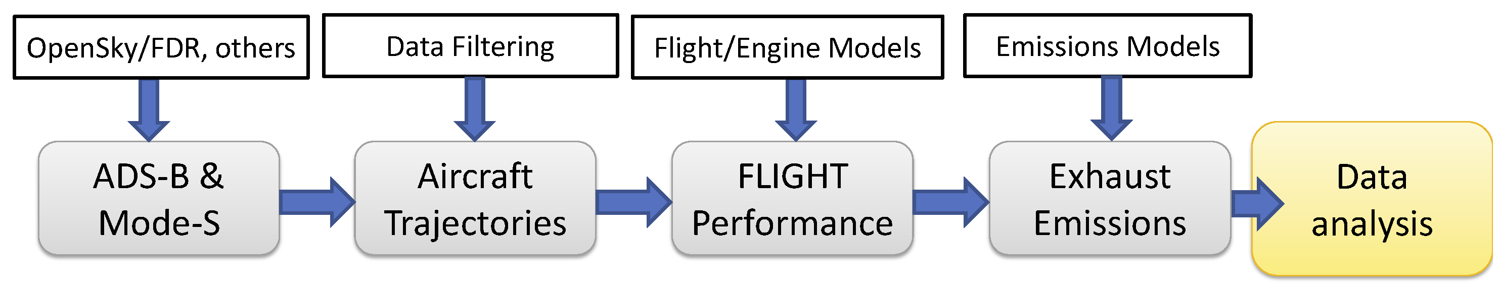
The data are used for the first category, and they are complemented with simulated data where there are gaps in the trajectory and in other aspects of the flight, including atmospheric temperatures, gross weights, and true airspeed. All engine parameters, in the second category, are entirely simulated, and so is the emissions modelling. The complete approach is described by the flowchart in Figure 1.
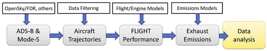
Figure 1.
Integration of ADS-B flight data to determine exhaust emissions from real-time flights.
The initial and final coordinates are used to identify the origin and the destination airport from an ancillary database of world airports (with the exception of helicopters, which can operate from/to unrecognised locations). With this further database, we can identify national and international flights.
Raw ADS-B/Mode-S trajectories need a considerable amount of mathematical filtering in order to make them usable for flight performance simulation. Typical operations include resampling, filtering, and removal of anomalies such as NaN; these can be either removed outright or filled in with average data between suitable data points.
Several mathematical techniques have been developed to clean up these trajectories; various algorithms have been implemented to identify features such as U-turn on departure or arrival, loitering/hold, aborted landing and go-around, and en-route stop. These techniques are demonstrated in [6]. For example, an en-route stop is detected from the condition
subject to the value of Equation (1) being maintained for a minimum amount of time, for example, 5 min. This is important also for helicopter flight, which determines either a hover of a landing condition. If the flight altitude z has a local minimum at the point of minimum gradient, then it is likely to be a landing; otherwise, it is defaulted to hover. Equation (1) can be modified using a digital elevation model to identify ground level, in which case it will be easier to identify en-route landing.
A loop or loiter is detected from a condition of continuous turn, which is derived from the heading angle
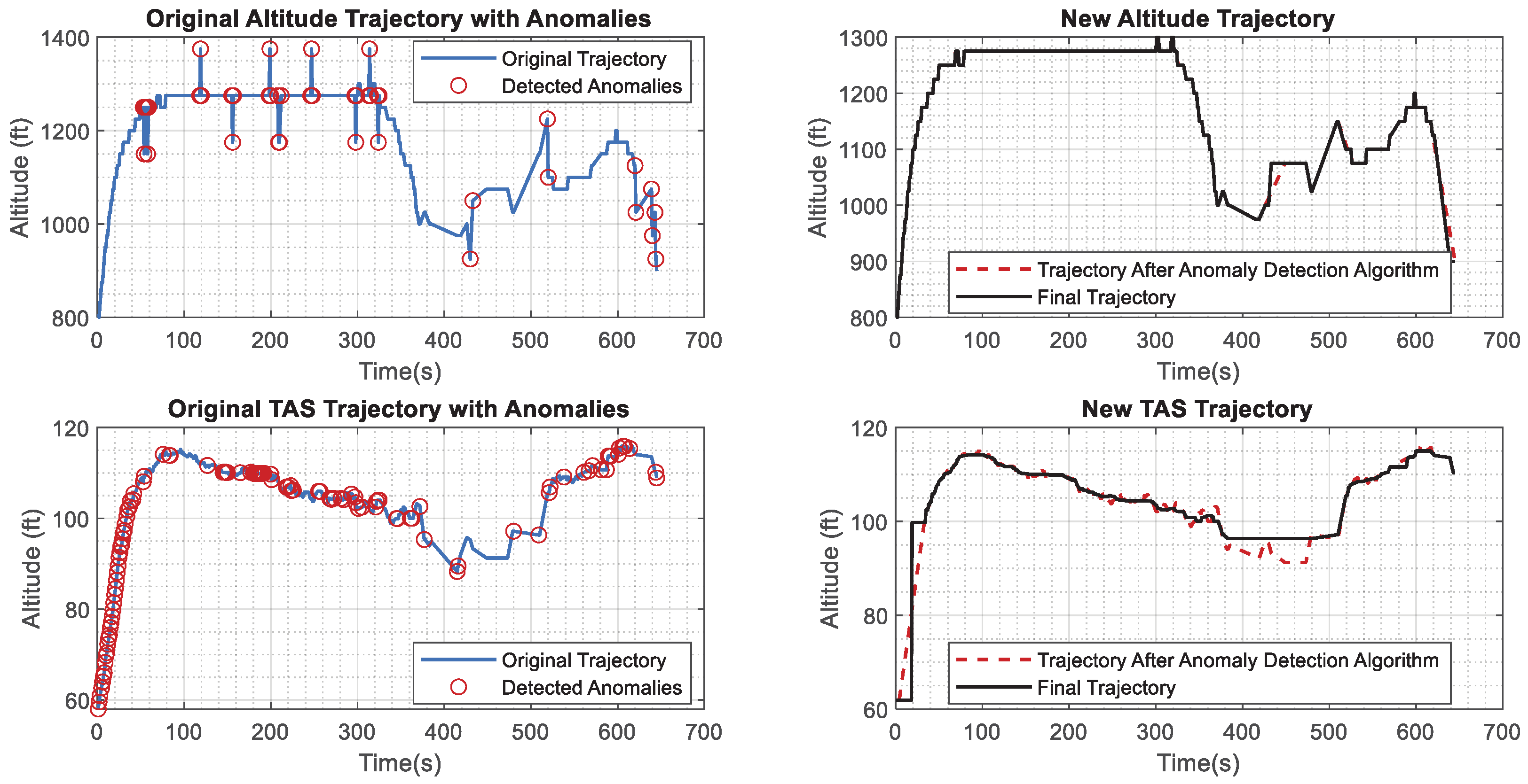
Filtering is a necessary tool, particularly when considering the effects on the climb or descent rates. Since the data are too coarse, climb/descent rates show unrealistic fluctuations. There are several techniques to remove these oscillations, first by central differencing, then by using low-pass filters, one of which is the Savitzky–Golay filter. Other techniques that have been applied include machine learning. One such application is shown in Figure 2.
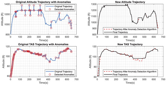
Figure 2.
ADS-B flight trajectories of a Eurocopter AS350-B3.
ADS-B/Mode-S data are by themselves insufficient, as in most cases the landing-and-takeoff phases are not stored. These flight segments are important, particularly for short flights, and are thus simulated to fill in the gaps. A full trajectory analysis is integrated with the missing flight segments, and includes taxi-out, take-off, and climb-out to the first useful altitude from ADS-B/Mode-S data; then, final approach from the last available ADS-B/Mode-S point, descent, landing, and taxi-in. The numerical methods for these phases are described in [8]. The initial and final altitude of the ADS-B data depends on the region of the world. Europe is well covered, but data below 1000 feet are uncommon. Flight from/to US airports usually start and terminate at much higher altitudes (5000 to 7000 feet), which requires a considerable amount of simulation to complete the flight.
However, after these operations are carried out, there is the opportunity to investigate the flights into more detail to provide events such as U-turns, go-around, aborted landing, en-route stops, etc. Each flight trajectory is then parsed and “flown” with an independent performance/environmental simulation code, in order to estimate exhaust emissions such as CO, CO, uncombusted hydrocarbons, SO water vapor, particulate matter, and other chemical species. The data are stored in large databases that are then postprocessed in order to provide emissions estimates according to aircraft type, route, city-pairs, altitude distribution, and a large variety of other aggregations.
2.1. Aircraft Models
The main gaps in knowledge are the atmospheric conditions and the gross take-off weight. It has been previously demonstrated [9] that particularly for long range, the required range is a better discriminator than take-off weight when it comes to estimating emissions. Therefore, we use the following estimate for the weight W:
where ZFW is the zero-fuel weight, is the airplane fuel capacity, X is the required range, and is the airplane’s design range. Equation (3) would imply that the aircraft cannot fly beyond its design range, which is not correct; nevertheless, the equation is useful in estimating the gross weight within the scope of this application. The value of X is found from the evaluation of the flight track between origin and destination airports—it is not the great-circle distance.
Next, it is necessary to estimate the thrust required in a quasisteady flight. This is done through the dynamics equation
where D is the total aerodynamic drag calculated following the methods in [10] at air speed V; is the acceleration, is the climb or descent rate. This derivative is estimated from the filtered ADS-B data; further averaging may be required over a time step of 20 ÷ 30 s in order to avoid unrealistic oscillations of this flight parameter. Unrealistic climb rates will reflect in undeliverable thrust or power.
A further improvement on Equation (3) is to iterate on the estimated weight. Since the loaded weight is a sum of payload and fuel, the latter item is calculated on a first run of the trajectory, and in a second iteration is used to compare the actual fuel burn with the initial estimate. For a helicopter, we have
where the last term is the power required to climb with climb rate ; and are the main- and tail rotor power, respectively. Finally, there are contributions from the gear-box and the airframe. It is further noted that in this case the aircraft is simulated in a quasisteady state. There are no accelerations in Equation (5). From the flight conditions, the rotorcraft is trimmed to fly the prescribed trajectory. A number of internal loops provide this trim, and ultimately, there is a power requirement . Rotor power requirements are calculated using a combined momentum theory and blade element theory with a rigid blade flapping dynamics. For the purposes of the calculation shown, flapping dynamics is not calculated in order to speed up the calculations; that has only a minimal effect on the required power but a large effect of the computations. For brevity, these models are not elaborated further.
From the net thrust or required power the fuel flow and other engine parameters are then calculated by simulating the aero-engine in reverse. This means that for a given flight state and a required net thrust or power, the model attempts to estimate the engine speed, the fuel flow, the aero-thermodynamic parameters at critical sections of the engines, as well as the chemical emissions, as discussed next.
2.2. Emissions Models
Within the context of engineering calculations of aero-engine emissions, the most practical method relies on the concept of emission index for each chemical species at selected values of engine outputs. For regulated aero-engines (turbofans with rated thrust 26.7 kN), these data are supplied (for reference only) by the ICAO Databank [11]. Although invaluable, these data must be used with caution. The standard calculation method in the European Environment Agency [12] still uses the ICAO reference points but does suggest three Tiers of calculations, one of which includes provisions for cases when the LTO operational data are not known.
The ICAO data are intended for engines on a test bench (hence static), at sea level and standard conditions. To extrapolate to actual flight conditions, a number of methods have been proposed, with the Boeing method being prevalent [13]. Corrections are introduced to take into accounts the effects of flight Mach number, altitude, and atmospheric humidity effects. With regards to the particulate emissions, the most recent version of the ICAO Databank [11] provides data at the standard operating points for some (not all) regulated turbofan engines. There is a gap in knowledge for nonregulated engines, which are treated statistically when no other modelling option exists [14]. The approach followed in our work is to use the ICAO emissions by default, and when these are not available, they are entirely modelled, in this instance using an implementation of the ImFox model [15]. The temperature in the combustor is extracted from the engine model that forms part of the overall simulation framework of the computer code FLIGHT. Temperature estimation was demonstrated recently on the Trent 970 turbofan engine [7].
3. Results and Discussion
The results are aggregated in a time-dependent calculation, and for each time step, there is a large variety of flight parameters. The outputs can be analysed in a great variety of ways—for example, by altitude (so we we would have LTO emissions, stratospheric emissions, and overall emissions), by required range, and by city pairs.
3.1. Commuter Airplanes
The ADS-B data have been used in order to investigate network issues, such as, for example, short commuting flights within Europe [6]. In this instance, we show selected results for the SAAB 340 turboprop, for which we analysed 894 ADS-B flights.
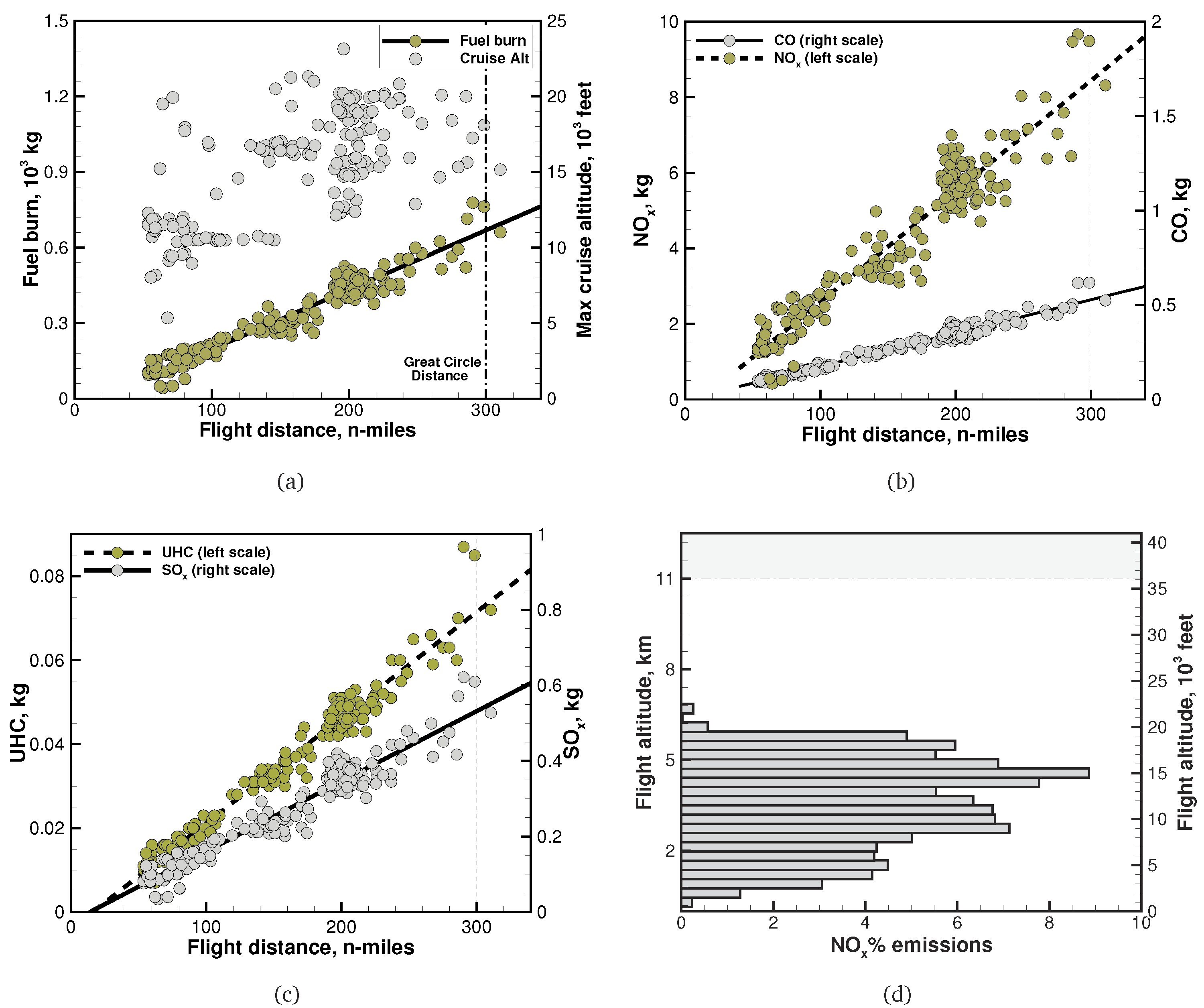
Figure 3 displays simulations for the SAAB 340 commuter turboprop operating across destinations in Europe. The emissions are aggregated by altitude, which is important when dealing with local air quality (flight altitudes < 3000 feet above ground). The largest concentration of NO is around 15,000 feet, although there is a wide spread of maximum altitudes shown in Figure 3a. In terms of fuel burn and emissions proportional to it, the actual flight distance is the clearest discriminator.
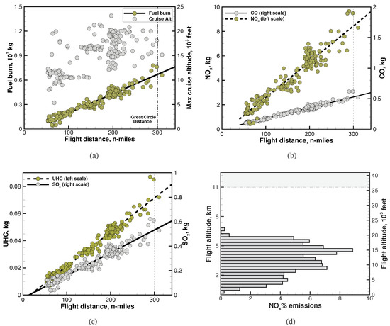
Figure 3.
Estimated fuel consumption and emissions for the SAAB 340 turboprop airplane, with analysis limited to 300 n-miles. All data are prepandemic. (a) Flight parameters; (b) Combustion emissions; (c) Combustion emissions; (d) Vertical distribution of NOx.
3.2. Wide-Body Long-Range Aircraft
The airplane considered was an Airbus A380. This wide-body airplane operates long-haul intercontinental flights, but one airline also operates some national feeder flights to pickup and disembark passengers. Intercontinental flights go over large shadow areas where there is no ADS-B coverage; that causes large blanks in the trajectory, which requires interpolation of data.
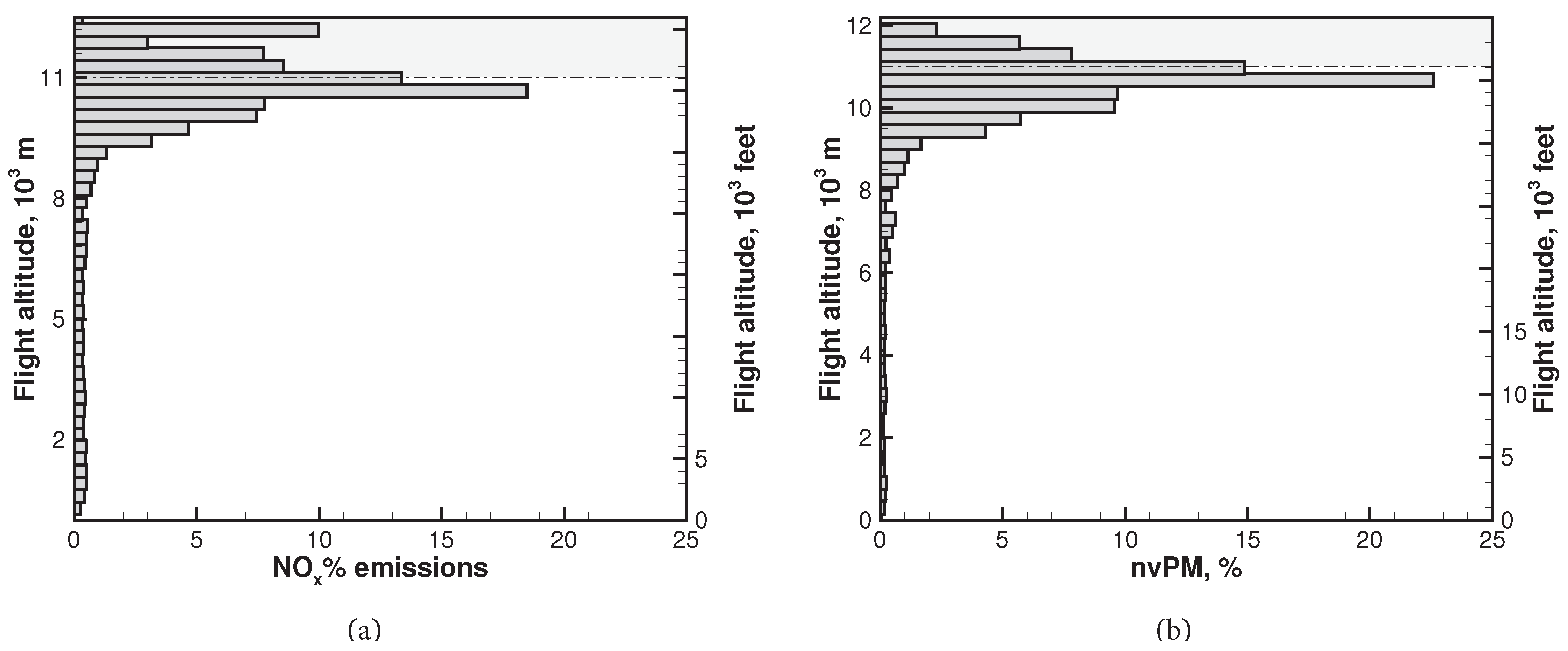
In our analysis, we considered a set of 509 flights, of which only 251 were representative enough to be suitable for simulation. This still required a direct simulation of the terminal-area operations, since these data are not recorded by the ADS-B data tracks. The analysis demonstrated that the 251 flights corresponded to a total 2582 total flight hours, with 1219 h of stratospheric flight. Selected emissions results are shown in Figure 4. One important observation to make is concerned with the altitude distribution of these emissions in comparison with a turboprop commuter airplane, Figure 3d.
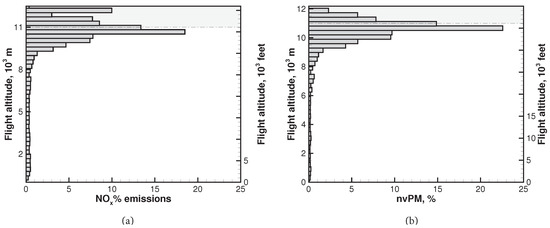
Figure 4.
Estimated altitude-dependent emissions for Airbus A380. (a) Flight altitude statistics; (b) Vertical emissions distribution.
One item of interest in long-range cruise is the amount of emissions at stratospheric altitudes. Stratospheric emissions have been investigated in some detail, and the available knowledge indicates that there are several environmentally complex effects, such as the NO depletion of atmospheric ozone, for example [16], increase in humidity levels at altitudes where there is limited recirculation, and possible climatic effects. Residence times of many chemical compounds is longer than in the lower atmosphere [17]. In this instance, there is a large concentration of NO and nvPM on or above the troposphere. Where the altitude effects are important [18], they are clearly demonstrated.
3.3. Business Jets
Business jets operate at the opposite end of the market just discussed. They service passengers over a wider range of destinations, from short haul to intercontinental, and a closer look at the flights distribution makes interesting reading indeed Figure 5.
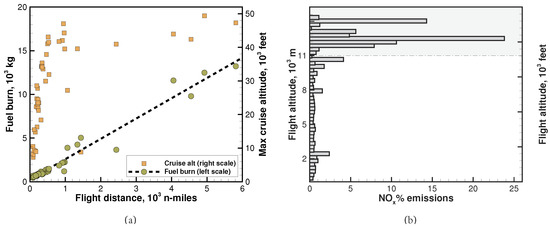
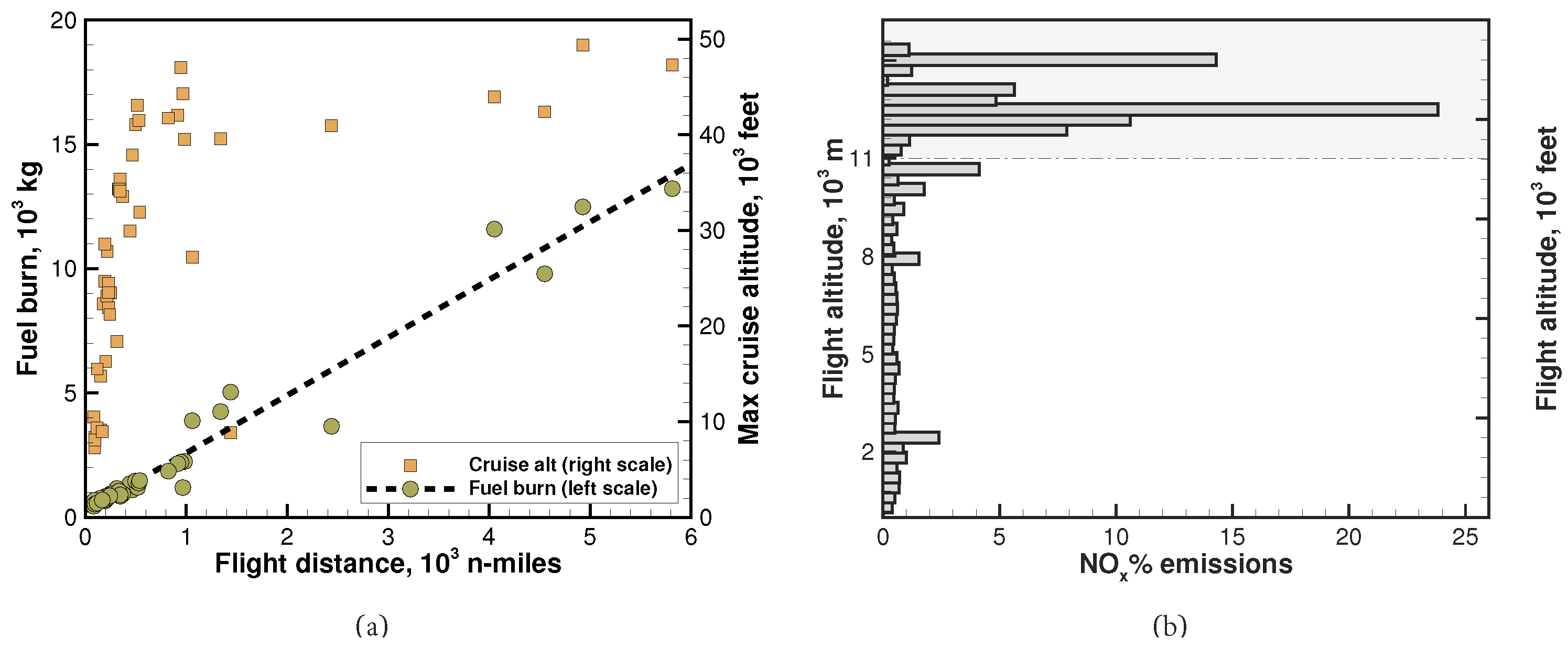
Figure 5.
Analysis of ADS-B flights and corresponding fuel burn for a Gulfstream G550. (a) Flight parameters; (b) Vertical emissions analysis.
One such analysis has revealed how a Gulfstream G550 has been used for services as short as HKG-SZX (Hong Kong to Shenzhen, return; 18 n-miles on the great-circle but 95 n-miles in practice at maximum altitude of 8000 feet) and GVA-SIN (Genéve to Singapore; 5667 n-miles at maximum altitude of 47,000 feet). For the shorter destination, official travel information indicates that the journey can be done by bullet train (15–20 min), private car (up to 1.5 h), scheduled ferry (up to 1 h), and even by coach. In any case, there is a relatively large number of short flights with correspondingly low cruise altitudes (bottom left of the Figure 5a). Most of the flights shorter than 300 n-miles are between European cities, one of which is a transfer between Moscow Sheremetievo and Moscow Vnukovo (23 n-miles).
Due to the great variety of flight profiles, CO emissions vary greatly, from 106 kg/n-mile to 7.35 kg/n-mile for a long range flight. For a GVA-SIN flight, the airplane spends ∼700 min at stratospheric altitudes, emits ∼39 metric tons of CO, ∼15.3 metric tons of water vapor, 52.87 kg of NO, 0.76 kg of nvPM, and discharges about 5.15 GJ of engine exhaust heat in the high atmosphere. The exhaust heat is calculated from the total mass flow rate and the exhaust gas temperature, which is calculated as part of the aero-thermodynamics of the engine. For all flights in Figure 5a, we identified over 49 flight hours at stratospheric altitudes. This airplane is capable of reaching altitudes of 50,000 feet above mean sea level, with correspondingly high stratospheric emissions, Figure 5b, in contrast to short commuters.
3.4. Helicopters
The helicopter model used to demonstrate the simulation models is the Eurocopter AS350-B3. Models for exhaust emissions of turboshaft engines are rather limited, and research in this area has been lagging in comparison with large turbofan engines. The only reliable assessment of emissions is the report by Rindisbacher et al. [19], where emission indices are estimated at a number of discrete points, with indices averaged across the turboshaft power outputs. The report cited is based entirely on empirical analysis. In fact, the emissions indices are only dependent on the shaft power. The fuel burn is calculated from
where i is the time-step counter. At each time step, we estimate the total shaft power from an aero-mechanic model of the helicopter. Given the flight condition , we trim the helicopter at that flight state, calculate the total power P, and then we solve the turboshaft problem in inverse mode (as in the previous case). This step yields the fuel flow , the engine speed, and other parameters. From the shaft power, we also determine the emission indices for CO, UHC, NO and particulate matter following the empirical relationships in [19].
It is essential to have ADS-B trajectories that are sufficiently clean (see Figure 2) because any unrealistic accelerations and climb rates will result in power requirements that cannot be delivered, Equation (5); this causes the simulations to be halted.
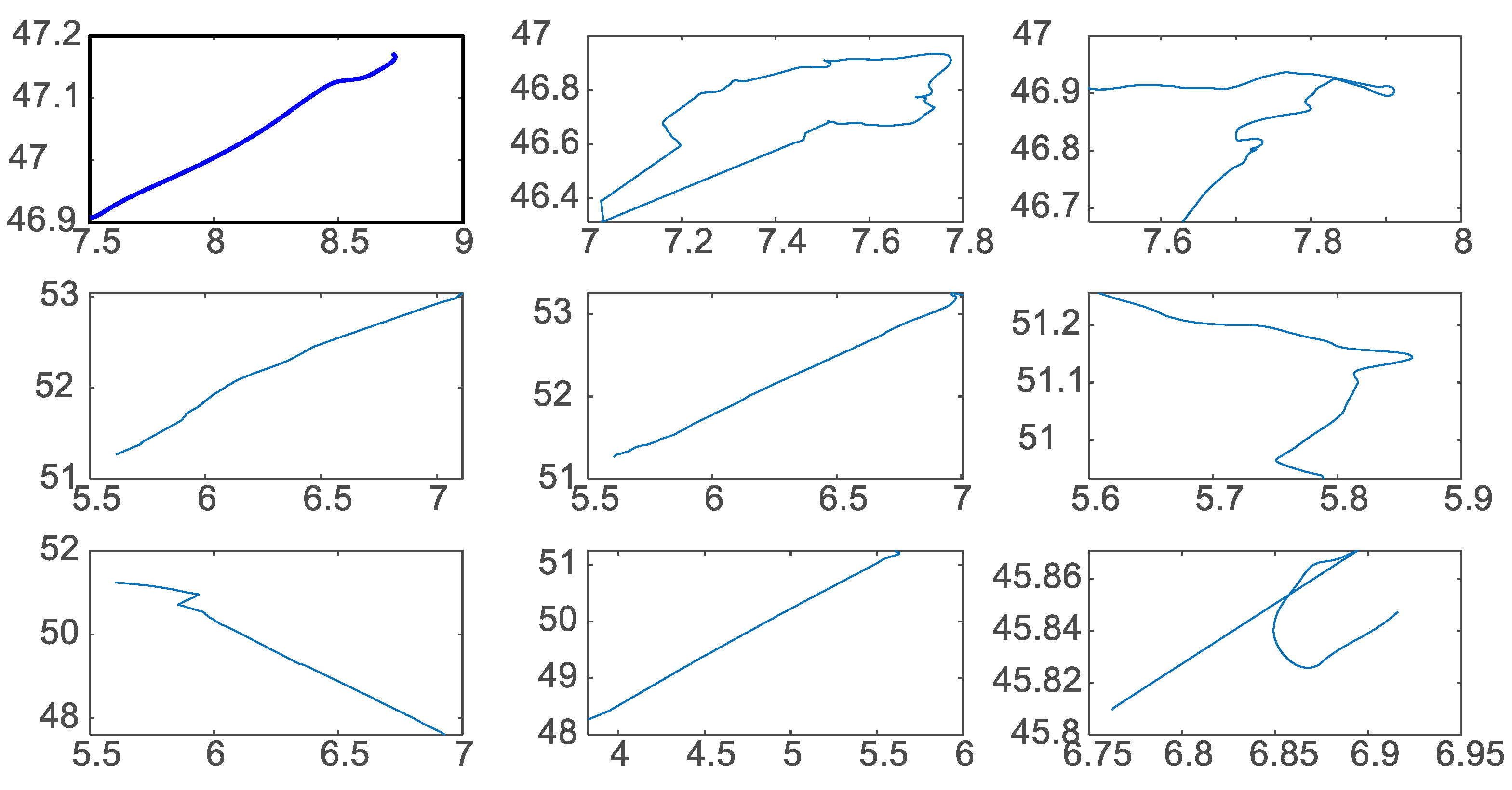
The test case is that of a single-engine Eurocopter AS350-B3 (now Airbus H125) powered by a Turbomeca Arriel 2B1 turboshaft. This engine is rated at 543 kW maximum continuous power (new, uninstalled, static sea level). Each flight is different, and data aggregation is not possible. In fact, a large set of flight tracks (not shown here) contain a considerable amount of loops and hover, possibly associated to police operations. An example is shown in Figure 6. Only the flight in the top left of Figure 6 is considered.
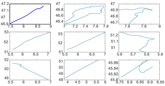
Figure 6.
Selection of ADS-B flight tracks of the AS350-B3 helicopter. The labels on the horizontal and vertical axis represent longitude and latitude in degrees, respectively.
The algorithm used to filter out trajectories that have too many loops and crossovers uses a MATLAB function called InterX to compute the locations where the trajectory has self-intersections and their corresponding number. However, a separate investigation can be carried out on the database to identify the type of operations, altitude distributions, hover performance, and so on.
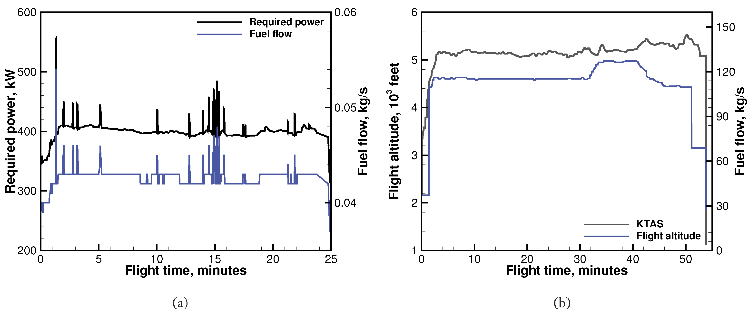
For the reference flight, the estimated chemical emissions are ∼1.37 kg of CO, ∼0.72 kg of NO, ∼1.04 kg of UHC, and ∼0.022 gr of nvPM. The estimated fuel burn was 255 kg, corresponding to ∼806 kg of CO over a flight time of 55 min. Simulated trajectory data are shown in Figure 7. It is noted that throughout the flight the power requirements are well within the limits of the engine power rating for this helicopter.
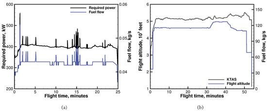
Figure 7.
Simulated flight parameters of an AS350-B3 helicopter from Figure 6. (a) Flight Power; (b) Flight parameters.
4. Conclusions
We reported a series of models that in combination with OpenSky ADS-B/Mode-S flight data can be used to estimate emissions from a variety of aircraft powered by gas turbine engines. We demonstrated the methods for a commuter turboprop, a long-range business jet, and a general utility aircraft. The models proposed require considerable filtering of the flight data, a flight mechanics model, a propulsion model with fuel flow with chemical emissions, atmospheric conditions, and a variety of other ancillary models in order to fill in the gaps in the data and aircraft performance. Although the results are not independently verified, which requires at least a comparison with FDR data with fuel flow values, they are demonstrated as reasonable and credible. We are able to identify several features of the flight and a large number of anomalies, and we can produce environmental analysis at a detailed level. To understand emissions, data must be averaged over a large number of flights, or between city pairs, and possibly also across different seasons in order to understand weather effects. These are important and require separate databases.
The results for helicopter flight deserve a special mention. The simulation models and the ADS-B data are currently too approximated to be considered reliable, and considerable efforts are needed in both modelling of turboshaft engine emissions and higher quality ADS-B trajectories.
Author Contributions
A.F. conceived the work, carried out the simulations with FLIGHT-X and FARP computer codes, analysed the data and produced the figures; S.M. processed the helicopter raw data and provided machine learning techniques to clean up the ADS-B trajectories used for the simulation (Section 3.4); B.P. wrote interface codes to extract and analyse ADS-B data from the OpenSky repository, produced an interface with the FLIGHT-X code and co-wrote the paper; N.B. analysed all the data and co-wrote the paper. All authors have read and agreed to the published version of the manuscript.
Funding
This work was sponsored by the UK Research Councils, EP/S010092/1 and by the Ekpe Research Impact Fellowship in the Department of MACE.
Data Availability Statement
Research data will be supplied on request, provided they will not be intended for commercial use.
Conflicts of Interest
The authors declare no conflict of interest. The funders had no role in the design of the study or in the collection, analyses, or interpretation of data.
References
- Simone, N.; Stettler, M.; Barrett, S. Rapid estimation of global civil aviation emissions with uncertainty quantification. Transp. Res. Part D Transp. Environ. 2013, 25, 33–41. [Google Scholar] [CrossRef]
- Olsen, S.; Wuebbles, D.; Owen, B. Comparison of global 3-D aviation emissions datasets. Atmos. Chem. Phys. 2013, 13, 429–441. [Google Scholar] [CrossRef] [Green Version]
- Kim, B.; Fleming, G.; Lee, J.; Waitz, I.E.A. System for assessing Aviation’s Global Emissions (SAGE), Part 1: Model description and inventory results. Transp. Res. Part D 2007, 12, 325–346. [Google Scholar] [CrossRef]
- Lee, J.; Waitz, I.; Kim, B.; Fleming, G.; Maurice, L.; Holsclaw, C. System for assessing Aviation’s Global Emissions (SAGE), Part 2: Uncertainty Assessment. Transp. Res. Part D 2007, 12, 381–395. [Google Scholar] [CrossRef]
- Stettler, M.; Boies, A.; Petzold, A.; Barrett, S. Global Civil Aviation Black Carbon Emissions. Environ. Sci. Technol. 2013, 47, 10397–10404. [Google Scholar] [CrossRef] [PubMed]
- Filippone, A.; Parkes, B. Evaluation of commuter airplane emissions: A European case study. Transp. Res. Part D 2021, 98, 102979. [Google Scholar] [CrossRef]
- Bojdo, N.; Filippone, A.; Parkes, B.; Clarkson, R. Aircraft engine dust ingestion following sand storms. Aerosp. Sci. Technol. 2020, 106, 106072. [Google Scholar] [CrossRef]
- Filippone, A. Advanced Aircraft Flight Performance; Cambridge Univ. Press: Cambridge, UK, 2012. [Google Scholar]
- Filippone, A.; Parkes, B.; Bojdo, N.; Kelly, T. Prediction of Aircraft Engine Emissions using ADS-B Flight Data. Aeronaut. J. 2021, 125, 988–1012. [Google Scholar] [CrossRef]
- Filippone, A. Comprehensive Analysis of Transport Aircraft Flight Performance. Prog. Aerosp. Sci. 2007, 43, 192–236. [Google Scholar] [CrossRef]
- ICAO. The ICAO Engine Emissions Databank. Available in Electronic Format from the EASA Website. 2021. Available online: www.easa.int (accessed on 31 December 2021).
- Whinter, M.; Rypdal, K. EMEP/EEA Air Pollutant Emissions Inventory Guidebook; Technical Report; European Environment Agengy: København, Denmark, 2019; Sections 1.3.a and 1.3.b Aviation. [Google Scholar]
- Baughcum, S.; Tritz, T.; Henderson, S.; Pickett, D. Scheduled Civil Aircraft Emission Inventories for 1992: Database Development and Analysis; Technical Report NASA CR-4700; NASA: Washington, DC, USA, 1996; Appendix D. [Google Scholar]
- Filippone, A.; Bojdo, N. Statistical Model for Gas Turbine Engine Emissions. Transp. J. Part D 2018, 59, 451–463. [Google Scholar] [CrossRef] [Green Version]
- Abrahamson, J.; Zelina, J.; Andac, M.; Vander Wal, R. Predictive Model Development for Aviation Black Carbon Mass Emissions from Alternative and Conventional Fuels at Ground and Cruise. Environ. Sci. Technol. 2016, 50, 12048–12055. [Google Scholar] [CrossRef] [PubMed]
- Portmann, R.; Daniel, J.; Ravishankara, A. Stratospheric ozone depletion due to nitrous oxide: Influences of other gases. Philos. Trans. R. Soc. B Biol. Sci. 2012, 367, 1256–1264. [Google Scholar] [CrossRef] [PubMed] [Green Version]
- Forster, C.; Stohl, A.; James, P.; Thouret, V. The residence times of aircraft emissions in the stratosphere using a mean emission inventory and emissions along actual flight tracks. J. Geophys. Res. Atmos. 2003, 108, 8524. [Google Scholar] [CrossRef] [Green Version]
- Skowron, A.; Lee, D.; De León, R.R. The assessment of the impact of aviation NOx on ozone and other radiative forcing responses—The importance of representing cruise altitudes accurately. Atmos. Environ. 2013, 74, 159–168. [Google Scholar] [CrossRef] [Green Version]
- Rindlisbacher, T.; Classey, L. Guidance on the Determination of Helicopter Emissions; Technical Report; FOCA: Bern, Switzerland, 2015.
Publisher’s Note: MDPI stays neutral with regard to jurisdictional claims in published maps and institutional affiliations. |
© 2022 by the authors. Licensee MDPI, Basel, Switzerland. This article is an open access article distributed under the terms and conditions of the Creative Commons Attribution (CC BY) license (https://creativecommons.org/licenses/by/4.0/).