1. Introduction
Implementation of the PBN concept facilitated accurate aircraft navigation and sequencing along the dedicated route structures such as trombone and point merge procedures. The trombones are made of parallel segments, upwind and downwind, with a set of waypoints supporting path stretching, which helps to systematize the traffic flows to the runways [
1]. Point merge features the sequencing legs in the shape of arcs for path stretching, and was deployed recently in Oslo, Dublin and other airports around the globe [
2].
Evaluation of flight efficiency, and in particular, performance within the Terminal Manoeuvring Area (TMA), has been a topic of interest in recent years. International Civil Aviation Organization (ICAO) proposed a set of metrics to enable analysis of TMA performance [
3]. EUROCONTROL developed the methodology used by its Performance Review Unit (PRU) for the analysis of flight efficiency within the areas of safety, capacity, cost-effectiveness and environment, reflected in the yearly assessment reports, reviewing the flight inefficiency at the top 30 European airports [
4]. In addition, EUROCONTROL Innovation Hub (formerly the Experimental Centre) proposed a set of metrics specifically developed for detailed evaluation of the arrival sequencing, metering and spacing [
5,
6].
In this work, we adopt and extend the performance measurement techniques developed by EUROCONTROL, to capture horizontal and vertical flight inefficiency and quantify their effect on fuel consumption, as well as to evaluate the sequencing and metering at three European airports operating different arrival techniques.
2. Airports
The three airports selected for this study—Dublin (EIDW), Stockholm-Arlanda (ESSA) and Vienna (LOWW)—have a similar number of yearly movements, between 220,000 and 260,000. The three corresponding states publish their respective Aeronautical Information Publications (AIPs) in open access [
7,
8,
9].
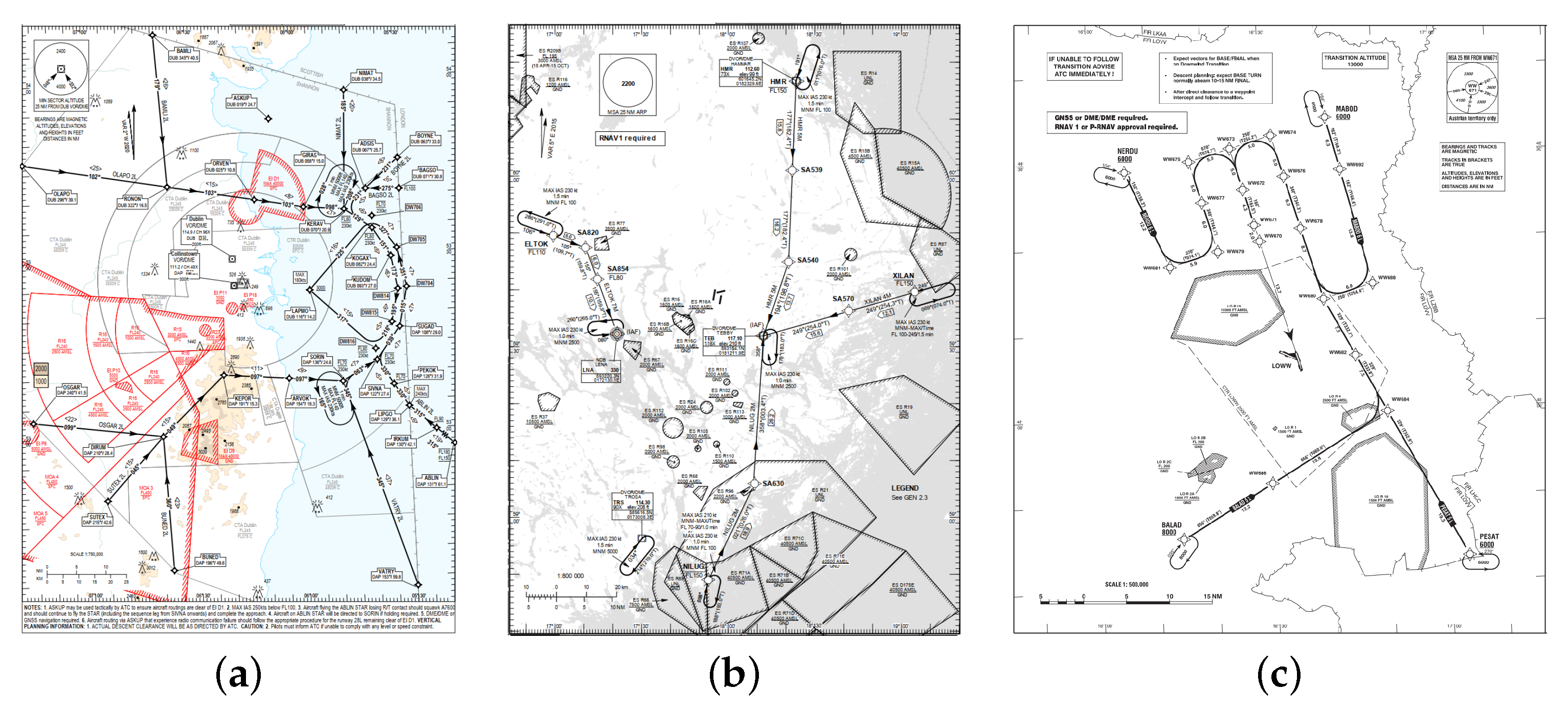
Dublin has two intersecting runways, but since runway 16/34 is only used for 5% of the aircraft movements, Dublin can be considered a single-runway airport. Dublin operates point merge procedures for both directions to its main runway 10R/28L (
Figure 1a [
7]), designed to work in high traffic loads without radar vectoring, and consists of a merge point and a set of sequencing legs flown at level, used for path stretching, before the aircraft are instructed to go directly to the merge point.
Arlanda has three runways, and most of the times, one runway is used for takeoffs and another for landings. The parallel runways is the preferred pair during peak hours and the capacity is 80 movements per hour. Arlanda operates a mix of closed STARs that connect all the way to the final approach, and open STARs, that require vectoring by the air traffic controllers from the Initial Approach Fix (IAF) to the final approach. The only runway not having a closed STARs system is 01R/19L (
Figure 1b).
Vienna has two intersecting runways that are used simultaneously to split the departures and arrivals. Vienna operates a set of STARs that lead to one out of four IAFs, shared by all four runways. From each IAF, a trombone transition connects to the final approach (
Figure 1c). The waypoints in the trombone system are used to adjust the path of the aircraft, in order to achieve the desired sequencing and separation.
For this study, at each airport we choose the runway that was used most in October 2019: 01R for ESSA (33% of the arrivals), 16 for LOWW (44%) and 28L for EIDW (80%). We evaluate the arrival procedures inside the TMA for Stockholm-Arlanda and Vienna airports. We noticed that a significant part of the eastbound flights to Dublin are cut by the TMA border with the descent starting significantly earlier than the time at which the aircraft enters the TMA, which may distort the arrival performance. Therefore, we extended our area of interest for Dublin to a 50 NM circle centered at the runway. For simplicity, the 50 NM circle area around Dublin airport will still be referred to as TMA.
3. Datasets
In this work, we use the historical database of the OpenSky Network [
10,
11]. We downloaded ’states’ data representing the parts of the arriving flight trajectories within ESSA, LOWW, and EIDW airport TMAs. We consider the year 2019 and select four full weeks in October, which was the month with the highest number of arrivals at the three airports (8797 arrivals at Dublin, 8132 at Arlanda, and 9625 at Vienna airport). The Opensky Data provides high-quality records and contains very accurate and detailed information about the aircraft movements. The information about the horizontal and vertical position of each aircraft is given in one-second time steps, which facilitates fine-grained evaluation and makes it possible to capture even small-scale inefficiencies in traffic flow.
A set of methods has been chained to perform a general cleaning of the trajectories:
Determine incorrect latitude or longitude (more than 0.1 degree distance from the previous record), fix all incorrect latitudes and longitudes using linear interpolation between the correct values
Substitute fluctuations in altitude (more than 300 m up and more than 600 m down) with the previous value
Use Gaussian filter to smooth the altitude
Remove the trajectories for which latitude, longitude or altitude could not be fixed by means of the previous steps
Remove the flights that go too far from the TMA border (more than 0.5 degree of latitude or longitude)
Remove the trajectories that are incomplete within TMA and do not reach the runway (last altitude is larger than 600 m)
Remove the trajectories which start from an altitude lower than 600 m (departure and arrival at the same airport, mostly helicopters)
Remove trajectories which represent landings too far from the runway (detected visually)
Remove trajectories, representing the go around within TMA (detected visually)
In addition, we removed trajectories with the following callsigns (representing mostly non-commercial flights):
Consisting of only letters (e.g., Swedish police helicopters: SEMIX, SEXTD, SEJPN, SEJPX, SEJPO)
Consisting of only digits
Shorter than four symbols (e.g., C33—Austrian air rescue helicopter)
Starting with DFL (Babcock Scandinavian Air Ambulance)
Starting with SVF (Swedish Armed Forces)
Starting with HMF (Swedish Maritime Administration)
The following datasets were created for the different types (large-scale and fine-grained) of the performance analysis.
PM Dataset consists of the flights adherent to the point merge procedures at Dublin airport. To create the dataset we filtered out the trajectories which either enter the TMA too far from any entry point (not within 0.5 degree radius), or which do not pass through either SIVNA or KOGAX waypoints (
Figure 1a) at the ends of the sequencing legs (with a catchment area of 0.5 degree radius around the point). The resulting PM dataset contains 3466 flights (45% of all the flights landed at runway 28L) adherent to the point merge procedures.
TB Dataset consists of the flights performing trombone procedures at Vienna airport. We select the trajectories passing either through the waypoint WW680 or the following pairs along the trombone structure (
Figure 1c): WW681 and WW679, WW692 and WW678, WW677 and WW672, MABOD and WW692, WW692 and WW688, WW692 and WW676, WW692 and WW672. The resulting TB dataset contains 1681 flights, which constitutes 40% of all the flights landed at runway 16 at Vienna.
TT Datasets represent the peak time periods and contain all arrivals corresponding to the hours when aircraft spent significantly long periods of time in TMA in average. We calculated the average per hour time in TMA and removed the 0.7th percentile from this set of values. The resulting datasets contain 2587 flights for Dublin, 1045 for Arlanda, and 1641 for Vienna.
Small Datasets. For the fine-grained evaluation of the arrival procedures, we choose smaller subsets from the corresponding TT datasets for each of the three airports, containing all the flights entering the TMAs during the chosen one-hour period. Two types of the small datasets are chosen: busy and the most delayed hours. For the busy-hour subsets we choose example hours with significant number of flights close to the maximum per hour, but similar for all three airports. In addition, we make sure that there were no significant weather events during these hours, to exclude the impact of weather on arrival flight efficiency. The idea is to see how the airports with different TMA complexities and arrival procedures handle similar amount of traffic per hour. The busy hours are: 4 October, 16:00–17:00 for EIDW with 32 arrivals, 3 October, 18:00–19:00 for ESSA with 33 arrivals, and 17 October, 17:00–18:00 for LOWW with 33 arrivals.
For each airport we also choose the most delayed hour by the maximum average time aircraft spent in TMA. For EIDW it was 1 October, 12:00–13:00 (32.15 min), for ESSA—15 October, 14:00–15:00 (23 min) and for LOWW— 13 October, 7:00–8:00 (29.58 min).
4. Methodology
We adopt a set of performance metrics developed by Eurocontrol PRU and Innovation Hub (formerly Experimental Centre) [
3,
5,
6], and extend the fine-grained analysis previously applied to Stockholm-Arlanda airport in [
12].
Additional Distance. We evaluate the horizontal flight efficiency using the Additional Distance in TMA. For that we cluster the trajectories in each TMA using the methodology proposed in [
13]. Next, we choose an ideal reference trajectory, constructing a user-preferred route tree inside the TMA as proposed in [
14]. We identify the start of the reference trajectory as the point on the TMA border that is closest to each cluster centroid. The reference trajectory goes directly to the interception of the localizer for an ILS approach, with a 2 NM straight segment before the Final Approach Point (FAP).
Time Flown Level. We use Time Flown Level in TMA to evaluate the vertical flight efficiency, calculated using the technique proposed by EUROCONTROL in [
5] with small changes. We identify the point of the trajectory where the aircraft enters the TMA and use it as a starting point. We identify a level segment when the aircraft is flying with the vertical speed below 300 feet per minute for at least 30 s, and these 30 s are subtracted from each level duration as suggested in [
5]. Flights under 1000 feet, corresponding to the final approach, are not considered as level flights.
Additional Fuel Burn. To evaluate the environmental efficiency of the arrivals we calculate the Additional Fuel Burn as the difference between the fuel consumption of the real and the reference trajectory corresponding to the CDOs. For the real flights, we use the TEM from BADA v.4.2 [
15] to find the thrust force, from which we derive the thrust coefficient. We also use BADA methodology to estimate the idle-thrust Continuous Descent Operations (CDOs) for all individual flights using the horizontal distance along the reference trajectory of the corresponding cluster. We take into account temperature and wind at the current position, obtained from ERA5 [
16]. The methodology is detailed in [
17]).
Minimum Time to Final. We plot all the flown trajectories of the given dataset and overlay a rectangular grid with the cell side of ≈ 1 NM, over the TMA and calculate the minimum time needed from any point within the cell of the grid to the final approach along any of the aircraft trajectories passing through the cell. We assign infinite (or a very large) value to the cells through which no trajectories pass during the considered time period. For visualisation of the resulting assignment, we plot a heatmap of the minimum time to final on a grid.
Horizontal Spread. We introduce this metric to roughly estimate the percentage of the TMA area occupied by the flights and quantify the dispersion of the arrival flows. It is calculated as the ratio of the number of cells through which at least one trajectory passes to the total number of grid cell covering the TMA. A smaller Horizontal Spread indicates that the aircraft mainly follow similar arrival paths.
Spacing Deviation. The spacing of an arriving aircraft pair at time
t is defined as the difference between the respective minimum times to final. The Spacing Deviation (
) at time
t is calculated for a pair of aircraft tagged as the leader and the trailer. The leader is the aircraft that arrives at the final point first, and the trailer is the aircraft that arrives second. The spacing deviation is calculated using the following equation:
where
is the temporal separation at the runway, and
min_time is the minimum time to final. The spacing deviation reflects information about the control error, i.e., the accuracy of spacing around the airport.
Throughput at a given time horizon, t is calculated by counting the number of aircraft with the minimum time to final within a given time window. In this work we calculate the throughput crossing iso-minimum time lines from 600 to 30 s to final, sampled at a 30 s rate over 5-min periods.
Metering effort is defined as the difference between the throughput at the given time horizon and the one close to the final (30 s in this work). It quantifies the controllers effort for metering, and may be used as a proxy to controllers workload.
5. Results
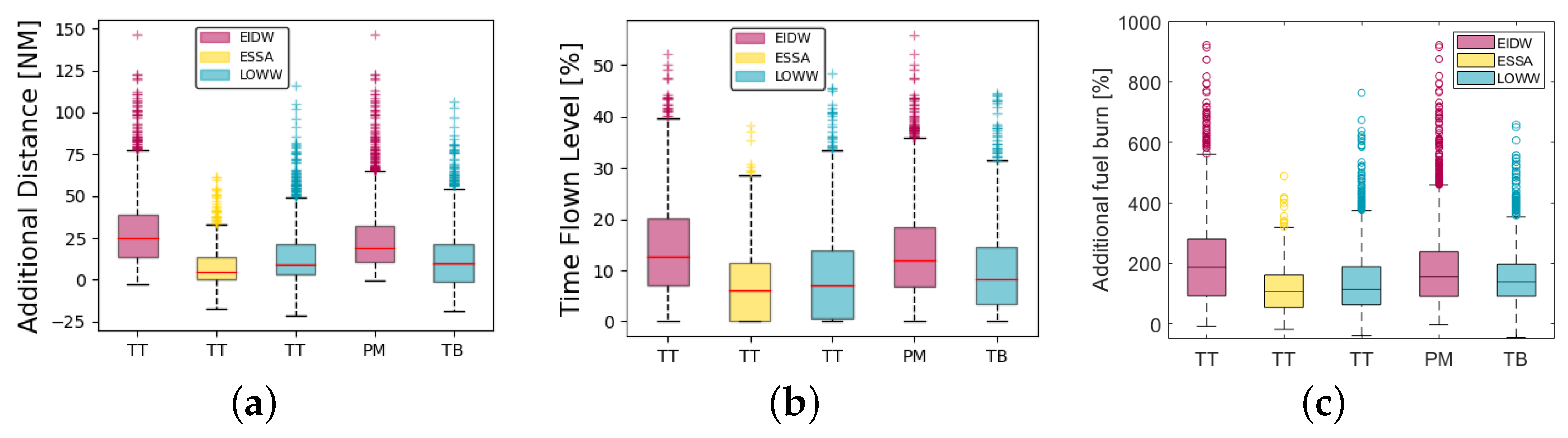
First, we perform a large-scale performance evaluation using the PM, TB, and TT datasets. The results illustrating the vertical, horizontal, and fuel performance statistics are shown in
Figure 2 (refer to
Figure 3a–c for clusters and corresponding reference trajectories). We can see that the Additional Distance calculated for TT datasets at EIDW is slightly higher than the one at ESSA and LOWW (the corresponding median values: 24.8 NM, 4.9 NM, and 8.8 NM), which results from the extensive use of the point merge arcs preceded by holding patterns for several flows. While the median values for this indicator are quite close for Arlanda and Vienna, the variation in the values is noticeably higher at Vienna. This fact can be explained by the systematic use of the trombone procedures, which extend the shortest direct routes at this airport. Similar disposition for the three airports is observed in the Average Time Flown Level (expressed in percent) and Additional Fuel Burn metrics, for the three airports (see
Figure 2b,c) with ESSA having the smallest median values (6.2 and 107.5%), slightly higher values for LOWW (7.1 and 114.1%), and the highest values at EIDW (12.7 and 186.8%).
Comparing the horizontal, vertical and fuel performance indicators calculated for the Dublin’s PM and TT datasets, we observe that adherence to the point merge procedures noticeably improves the performance (medians for Additional Distance: 19.5 vs. 24.9 NM, Average Time Flown Level: 11.9 vs. 19.5%, Additional Fuel Burn: 155.9 vs. 186.8%). The results of the comparison for Vienna’s TB and TT datasets revealed that while the medians for the corresponding performance indicators slightly increased (Additional Distance: 8.8 vs. 10.02 NM, Average Time Flown Level: 7.1 vs. 8.3%, Additional Fuel Burn: 114.1 vs. 138.3%) due to the adherence to the trombone procedures, the variance decreased.
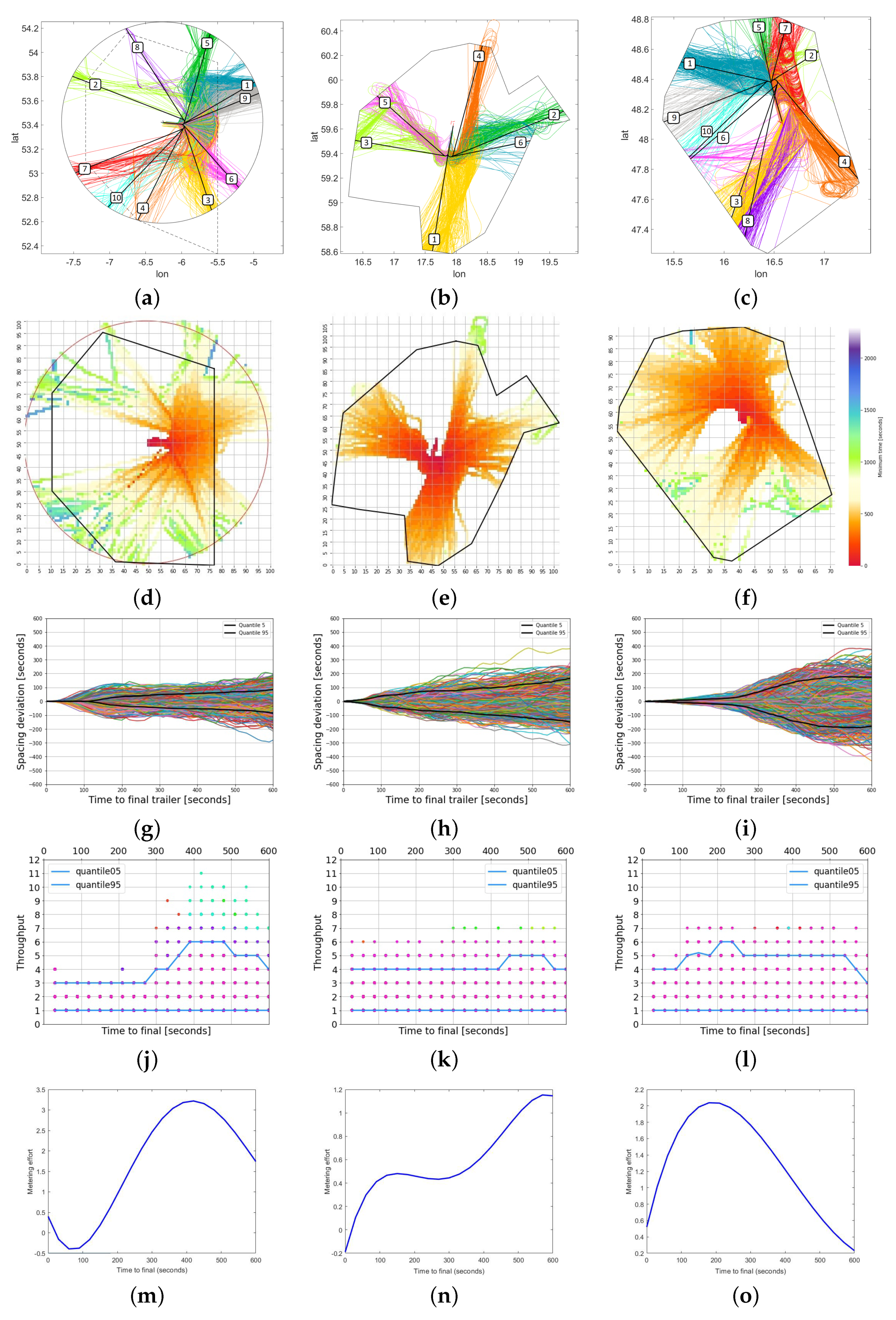
Figure 3 illustrates the results for the metering and sequencing performance metrics calculated for the TT datasets. These datasets are chosen for this kind or analysis because they contain all the flights during the peak periods at the airports (explained in
Section 3), in oppose to the PM and TB datasets composed of the selected flights only, and therefore not suitable for the analysis of the sequencing and spacing between consecutive aircraft.
Figure 3a–c show the aircraft trajectories at the three airports clustered according to the major flows. The Minimum Time to Final heatmaps (
Figure 3d–f) show higher maximum values of this metric for Dublin airport (2310 s) than the one for ESSA (1228 s) and Vienna (1524 s), which is consistent with the results obtained for the Additional Distance, and complement the horizontal efficiency evaluation. The corresponding Horizontal Spread for Dublin is 64%, indicating relatively low dispersion in the arrival flows which mainly follow the same paths, but with extra grid cells occupied by the holding patterns around at the starts of the sequencing legs. For ESSA, it is 59%, also suggesting a low flow dispersion, with the holding patterns organized quite far from the runway (around the entry points to TMA), leaving almost half of the airspace for in-flight trajectory changes and manoeuvres. For LOWW, the Horizontal Spread is around 84%, suggesting a larger area of dispersion, with possible effect in terms of area of attention for the controller, airspace availability for departures, and possible nuisance at low altitudes. Further analysis is required to understand the effects of the different horizontal spreads.
Spacing Deviation evolution curves illustrate how the spacing between aircraft pairs evolves in time (
Figure 3g–i), with a clear difference in the 90th quantile width (maximum difference between the %95 and %5-quantile values: 169 s for Dublin, 314 s for Arlanda and 365 s for Vienna) and time to final horizons when the flows start to converge to final: quite far from the runway at Dublin (around 450 s), much closer to the final at Vienna (200 s) and very smoothly through the whole approach at Arlanda. The shapes of the spacing deviation evolution curves, the Throughput and Metering Effort figures (
Figure 3j–o) show when the sequencing and metering effort is applied at each airport. For EIDW, the maximum Metering effort is observed at around 450 s time to final with the value exceeding 3. This value corresponds to a number of flights, and represents the difference of the spread (5–95% containment) of the throughput between 450 s and 30 s (final). The target throughput is reached when the metering effort is zero, here around 150 s. For ESSA, the maximum Metering effort is at 550 s with a value of 1.2. There is a first decrease up to 330 s and then the final one starting at 100 s with zero reached quite close to the runway. For LOWW, the Metering Effort goes up to 2 at around 200 s then decreases, almost reaching zero. The Metering Effort results indicate significant differences of entry conditions among the airports, with the traffic samples considered. Obviously, for a given airport, higher or lower traffic would lead to a different effort value. Here we may notice that EIDW is having by far the highest effort (3), followed by LOWW (2), and then ESSA (1.2). This should be taken into consideration when comparing flight efficiency.
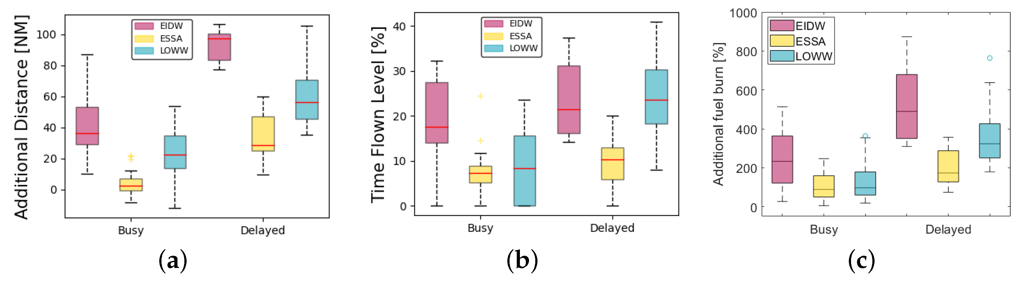
Figure 4 and
Table 1 summarize the results of the fine-grained performance evaluation for the busy and the most delayed hours at the three airports. Comparison of the horizontal and vertical performance during busy hour versus the corresponding results obtained for the large TT datasets, shows an increase in both the Additional Distance and Time Flown Level (in percent) for Dublin (36.4 NM and 17.5%) and Vienna (22.4 NM and 8.4%), increase in Time Flows Level for ESSA (7.4%), but some improvement in the Additional Distance at ESSA (2.7 NM). We can suppose that the aircraft at ESSA were following similar horizontal tracks during the busy scenarios. Additional Fuel Burn during the busy hours takes noticeably lower median values for Arlanda and Vienna (88.4% and 96.9%), and higher values for Dublin (232.6%).
All the three airports demonstrated a degraded performance during the most delayed hours, with high median values for Additional Fuel Burn (489.6% EIDW, 173.3% ESSA, and 323% LOWW), which result from the noticeably longer paths within TMA (97.4 NM EIDW, 28.8 NM ESSA, and 56.3 NM LOWW) and some increase in Time Flown Level (21.4% EIDW, 10.4% ESSA, and 23.6% LOWW). In general, all the airports seem to handle larger traffic intensities better than delays. While the disposition between the airports is the same for both scenarios, the arrival procedures at Arlanda tolerate the delays better than the other two airports with designated route structures. This fact is to be closer investigated in future work.
Examining the sequencing and metering indicators (
Table 1), we observe that Minimum Time to Final is also higher for all airports during the most delayed hours, which results from the fact that aircraft spent more time in TMA, following longer paths with a number of holding patterns (the corresponding figures are not provided due to space limitation). The Horizontal Spread is slightly higher during the busy than for the most delayed hours for all airports, which can be explained by higher traffic intensity during the busy hours resulting in rerouting patterns, with the lowest values observed at Dublin airport (where aircraft mostly follow similar tracks) and the highest at Vienna. Spacing Deviation captured via the widths of the 90th quantile, is slightly larger in Dublin and Vienna during the delayed periods, while at Arlanda it is higher during the busy hours. Controllers may decide to increase the spacing requirements, for example, when the delays are caused by extreme weather events. On the other hand, lower values of this performance metric during the delayed periods may be explained by the relatively low traffic intensity.
The maximum values of the Throughput and the corresponding Metering Effort are higher during the most delayed hours than during the busy hours at Arlanda and Vienna, and opposite for Dublin, indicating that the increase in traffic intensity increases the need for metering and sequencing actions during the corresponding hours.
6. Conclusions
In this paper, we evaluate the arrival flight efficiency of three European airports with different airspace complexity implementing different sequencing and merging techniques, but with similar amount of yearly movements. The analysis revealed varied situations among the three airports, with the medians for Additional Distance between 4.9 and 24.8 NM, Time Flown Level calculated in percent—from 6.2 to 12.7% and significantly high median values for Additional Fuel Burn (from 107.5 to 186.8%). Evaluation of arrival spacing and metering showed different pictures of horizontal spread of the arrival flows (from 59 to 84%), different metering efforts (from 1.2 at Arlanda to 3 at Dublin), as well as the times when the maximum control effort is applied. In addition, we observe that adherence to the designated route procedures significantly improved the efficiency at Dublin airport, while at Vienna the effect is slightly ambiguous, which is to be investigated in future work.
All the airports perform relatively better in the high-traffic scenarios than during the periods with high delays. An improved horizontal performance in congested scenarios was observed at Arlanda, as well as fuel efficiency at Arlanda and Vienna. In addition, Arlanda operations seem to cope better with the delays than the point merge and trombone procedures at the other two airports. However, no fair comparison is possible without considering the entry conditions to the terminal area. Further studies would be required to analyse flight efficiency under comparable entry conditions.


