A Hybrid Model of VAR-DCC-GARCH and Wavelet Analysis for Forecasting Volatility ^†

Abstract

The purpose of this study is to investigate the time-varying co-movement between the volatility of gold, exchange rate, and stock market returns in Iran, using weekly data from 27 September 2013 to 3 December 2021. The results of the wavelet-based random forest show that the performance of VAR-DCC-GARCH model is better than that of DCC-GARCH model in predicting financial market volatilities. Furthermore, the results of the VAR-DCC-GARCH model indicate that a positive and relatively high conditional correlation exists in the daily exchange rate and gold-return volatility. The conditional correlation is lower between the exchange rate–stock market returns and the daily gold–stock market returns. In short and long terms, there is no correlation between the exchange rate and the stock market volatilities as well as gold and stock market volatilities, while the correlation between the paired markets exists in the medium term.

1. Introduction

Among the important topics of financial economics are the modeling of volatility, the interdependence of volatility in financial markets, and forecasting. Volatility in financial markets occurs when these markets are at risk [1]. With the spread of information in financial markets, the correlation between markets and their volatility has increased. Investors predict price changes based on the price changes of other markets. In other words, an increase in the return of a market may change the return of the other markets at the same time. This change is called the “Spillover Effect”. Therefore, besides accurate modeling and forecasting of financial market volatility, examining their dependence can help investors, risk managers, and traders to create sustainable profits [2].

The exchange rate is determined by the trade balance or current account balance of countries. Since the exchange-rate changes affect international competition and trade balance, these changes affect real incomes and input prices. An increase in the input cost leads to a decrease in profit firms and a decline in stock price [3]. On the other hand, the exchange rate is determined by the supply and demand of financial assets such as equities and bonds, since expectations of relative changes in domestic currency have a significant effect on the price of financial assets. Bodnar and Gentry [4] show that the relationship between firm profitability and exchange-rate changes depends on the nature and type of industrial activity. An increase in the exchange rate leads to a decline in the price of exported goods in the importing country, and if demand is high in the importing country, the export rate will increase and the exporting company will benefit. Conversely, an increase in the exchange rate will make imported goods more expensive and reduce the value of the importing company (Unless the importer’s firms can transfer the price increase to the end consumer). The empirical literature provides conflicting findings of the dynamic relationship between the exchange rate and the stock market. Aggarwal [5], Kim [6], Doong et al. [7], and Dahir et al. [3] showed a positive relationship between the exchange rate and the stock market index. Erdogan et al. [8] showed that there were significant volatility spillover effects on the Islamic stock market to the foreign exchange market. According to Gavins [9] and Zhao [10], there is no relationship between exchange rates and stock prices. Hashim et al. [11] showed a negative relationship between the exchange rate and the stock market.

Since individuals hold their financial assets in a combination of cash, gold, currency, bonds, and equities, changes in each market can affect individuals’ investment portfolios. Rising inflation, exchange-rate fluctuations, or political instability can lead to some form of market excitement and increase demand for gold. Various studies have been conducted on the relationship between gold prices and stock indices, some of which are as follows: Gilmore et al. [12] showed that there is a cointegration between the gold price, the stock-market price of gold, and the US stock index. Mishra et al. [13] showed that there is no correlation between the gold price and stock index in India. Srinivasan [14] investigated the causal nexus between gold price, stock price, and exchange rate in India using ARDL. He showed that there exists no causality from gold price to stock price or vice versa in the short run. Arouri et al. [15] examine the relationship between the global price of gold and the Chinese stock market over the period of 22 March 2004 through to 31 March 2011 in China. For this purpose, they used VAR-GARCH and other multivariate GARCH models such as DCC and CCC. Their research results show that past gold returns play an important role in explaining the dynamics of conditional returns and stock-market volatility. Jain and Biswal [16], using a DCC-GARCH model, showed that falling gold and crude oil prices were causing the Indian stock market to decline. Yousaf and Ali [17] showed that there are return and volatility spillovers between the gold and emerging Asian stock markets during the global financial crisis. Moreover, several studies in the literature exist about the relationship between gold and the exchange rate. Sjaastad [18] found that since the dissolution of the Bretton Woods international monetary system, floating exchange rates among the major currencies have been a major source of price instability in the world gold market. Qureshi et al. [19] using a wavelet approach showed that gold acts as a consistent short-run hedge against the exchange rate. Wang et al. [20] argued that gold can partly hedge against the depreciation of the currency in the long run.

The purpose of this paper is to investigate the correlation between the volatility of gold, foreign exchange, and stock markets in Iran, using weekly average data from 27 September 2013 to 3 December 2021. For this purpose, this study compares two approaches, VAR-DCC-GARCH and DCC-GARCH, using out-of-sample evaluation by the wavelet-based random forest (WRF) model. Then, the co-movement of the volatility is analyzed using a continuous wavelet (CWT) in the timescale. Iran had been subjected to sanctions, a sharp increase in liquidity, and structural problems that caused inflation. Therefore, investors generally turned to invest in stocks, buying foreign currency, and gold. Given the increasing volatility in the underlying markets, this paper contributes to the literature on the Iranian financial market in the following ways:

• It shows whether a conditional correlation exists in the weekly exchange rate, gold, and stock market returns by using DCC-GARCH and VAR-DCC-GARCH.
• It reveals that performance of VAR-DCC-GARCH model is better than that of DCC-GARCH model using out-of-sample prediction by WRF.
• It identifies the time-varying nature of the correlation among the Iranian financial market’s volatilities indexes using CWT.
• This study helps investors identify the optimal portfolio by identifying asset-return volatility and portfolio diversification.

2. Materials and Methods

2.1. VAR-DCC-GARCH

In the VAR-DCC-GARCH model, the VAR method is used to estimate the conditional mean equation of the DCC-GARCH model. In this study, we consider the conditional mean equation VAR(1) according to the Schwartz and Akaike criterion. The conditional mean equation is written as Equation (1):

$$R_t=\mu +\mathsf{\Phi }{R}_{t-1}++e_{t}with{e}_t=D_t^{\frac{1}{2}}{\eta }_t$$

(1)

$R_t$ is the $4\times 1$ vector of returns of each variable, t is time, $\mu$ denotes a $4\times 1$ vector of constants, and $\mathsf{\Phi }=\left(\begin{array}{c}{\phi }_{11}\\ \begin{array}{c}{\phi }_{21}\\ \begin{array}{c}{\phi }_{31}\\ {\phi }_{41}\end{array}\end{array}\end{array}\begin{array}{c}{\phi }_{12}\\ \begin{array}{c}{\phi }_{22}\\ \begin{array}{c}{\phi }_{32}\\ {\phi }_{42}\end{array}\end{array}\end{array}\begin{array}{c}{\phi }_{13}\\ \begin{array}{c}{\phi }_{23}\\ \begin{array}{c}{\phi }_{33} \\ {\phi }_{43}\end{array}\end{array}\end{array}\begin{array}{c}{\phi }_{14}\\ \begin{array}{c}{\phi }_{24}\\ \begin{array}{c}{\phi }_{34}\\ {\phi }_{44}\end{array}\end{array}\end{array}\right)$ is a $4\times 4$ matrix of parameters measuring the influence of each variable with own-lagged and the other.$e_t$ is a residual of mean equation for four returns variables. ${\eta }_t$ indicates a $4\times 1$ vector of independenctly and identically distributed random vectors, and

$$D_t^{1/2}=diag\left(\sqrt{h_t^{oil}},\sqrt{h_t^{TEPIX}},\sqrt{h_t^{er}},\sqrt{h_t^{gold}}\right)$$

(2)

where $h_t$ indicate the conditional variance of returns variables. The conditional variance equation of the DCC-GARCH model is written as Equation (3):

$$H_t=D_{t}R{D}_t$$

(3)

The $H_t$ matrix is an MGARCH process that can be modeled using dynamic conditional correlation (DCC) [21,22]. According to Engel’s [21] model, a DCC model is defined as (4):

$$R_t=diag\left(q_{11 t}^{\frac{1}{2}}\dots q_{NN t}^{\frac{1}{2}}\right){\varrho }_{t}diag\left(q_{11 t}^{\frac{1}{2}}\dots q_{NN t}^{\frac{1}{2}}\right)$$

(4)

where ${\varrho }_t$ is the positive symmetric definite matrix of N × N and

$${\varrho }_t=\left(1-\mathsf{\alpha }-\mathsf{\beta }\right)\overline{\varrho }+\alpha u_{t-1}\acute{u_{t-1}}+\beta {\varrho }_{t-1}$$

(5)

$u_{it}=\frac{{\epsilon }_{it}}{\sqrt{h_{iit}}}$, $\overline{\varrho }$, a nonconditional variance matrix of ut, $\alpha$ and $\beta$ is nonnegative numerical parameters that satisfy $\alpha +\beta <1$.

2.2. Wavelet-Based Random Forest

In this paper, we consider wavelet-based random forest as a prediction approach. WRF is built based on maximal overlap discrete wavelet transform (MODWT) function and random forest algorithm learning approach. The model structure is flexible and efficient [23].

The wavelet-based random forest (WRF) is based on the method originally proposed by Breiman [24]. The WRF has two stages: The first stage is the bootstrap aggregation, or bagging samples, which is performed with two-thirds of the inputs. Second, for each node of the individual decision tree, a random selection of decision trees is chosen, and those variables belonging to the best split will be allowed to grow. To identify the best split, the Gini impurity function, first introduced by Breiman et al. [25], is used to minimize the effect of impurities and maximize homogeneity of the selected subsets. Each tree will undergo this process of selecting the best subset and minimizing impurity until it is halted by reaching the best possible training performance for each training process [26].

We use this model to be able to select the best model for evaluating volatilities. The WRF performances are measured with three error metrics including root-mean-squared error (RMSE), mean-squared error (MSE), and mean-absolute error (MAE).

$$MSE=\frac{1}{n}{\displaystyle \sum }_{i=1}^n{(O_i-P_i)}^2$$

(6)

$$RMSE=\sqrt{\frac{1}{n}{\displaystyle \sum }_{i=1}^n{(O_i-P_i)}^2}$$

(7)

$$R=\frac{{{\displaystyle \sum }}_{i=1}^n\left(O_i-O_{avg}\right)\times \left(P_i-P_{avg}\right)}{{({{\displaystyle \sum }}_{i=1}^n{(O_i-O_{avg})}^2 )}^{0.5}\times {({{\displaystyle \sum }}_{i=1}^n{(P_i-P_{avg})}^2 )}^{0.5}}$$

(8)

$$MAE=\frac{1}{n}{\displaystyle \sum }_{i=1}^n\left|O_i-P_i\right|$$

(9)

2.3. Continuous Wavelet Analysis

Continuous wavelet transform is a method used to investigate the relationship between two time series. In mathematics, a continuous wavelet function for the time series xt whose integral is squared, is defined by the scale a > 0 and the place B∈R as relation (10):

$$X\left(a,b\right)=\frac{1}{\sqrt{a}}{{\displaystyle \int }}_{-\infty }^{\infty }x\left(t\right){\psi }^{*}\left(\frac{t-b}{a}\right)dt$$

(10)

In this relation, $\psi \left(t\right)$ is a continuous function in both time and frequency domains. We use Morlet wavelet to define the $\psi \left(t\right)$ function as follows:

$${\psi }^M\left(t\right)=\frac{1}{{\pi }^{\frac{1}{4}}}\left(e^{i\omega t}-e^{-\omega /2}\right)e^{-t/2}$$

(11)

where ${\psi }^M\left(t\right)$ is the continuous Morlet function, t is time, and $\omega$ is frequency.

3. Discussion

The study employs weekly data on the Tehran Price Index, gold price, and Unofficial Free Exchange Rate (US Dollar) in the period from 27 September 2013 to 3 December 2021. The weekly return of the above variables can be defined as follows:

$$y_t=100 \left[\ln (p_t)-\ln (p_{t-1})\right]$$

(12)

where pt represents each variable under study. The descriptive statistics for the return series are shown in

Table 1. Descriptive statistics.

	TEPIX	USD	Gold
Mean	0.87	0.5507	0.636
Maximum	15.71	16.80	15.88
Minimum	−10.74	−10.87	−11.71
Sd	3.29	2.96	3.12
skewness	0.91	1.28	0.85
kurtosis	6.51	10.22	7.59
Jb	260.08	976.08	399.15

. Accordingly, the mean returns on TEPIX, USD, and gold are 0.87, 0.55, and 0.636, respectively. All of the returns series exhibit positive skewness and asymmetry. According to the Jarque–Bera test, the null of normality is strongly rejected for all returns series.

The results of Pearson’s correlation coefficient are shown in

Table 2. Pearson’s correlation coefficient.

	Gold	Dollar	TEPIX
gold	1
USD	0.777	1
TEPIX	0.1899	0.1552	1

. Accordingly, the unconditional correlation between the returns on TEPIX–USD, TEPIX–gold and USD– gold returns are positive. Since this analysis is straightforward and does not consider the effect of time on the correlation between the series of returns, the conditional correlation method is used.

This study employs the VAR-DCC-GARCH and DCC-GARCH method to calculate the volatility of all returns. In order to estimate VAR-DCC-GARCH, it is necessary to determine the optimal lag. In this research, it is chosen a VAR(1) for the mean equation using Akaike and Schwartz Bayesian criteria. The results of this estimation model are reported in

Table 3. Determination of optimal Lag.

	Akaike	Bayes	Hannan-Quinn
1	13.045	13.305	13.148
2	13.092	13.442	13.231
3	13.151	13.591	13.325

.

The results of estimating the mean equation are presented in

Table 4. Estimates of conditional mean VAR-DCC-GARCH model.

		Coefficient	p-Value
TEPIX	$c_1$	0.327	0.02
	${\phi }_{11}$	0.5058	0.000
	${\phi }_{12}$	0.087	0.24
	${\phi }_{13}$	−0.005	0.94
USD	$c_2$	0.362	0.000
	${\phi }_{21}$	0.0678	0.000
	${\phi }_{22}$	−0.0591	0.000
	${\phi }_{23}$	0.2856	0.000
gold	$c_3$	0.470	0.003
	${\phi }_{31}$	0.1376	0.004
	${\phi }_{32}$	−0.097	0.23
	${\phi }_{33}$	0.1924	0.01

. ${\phi }_{11}$, ${\phi }_{22}$, ${\phi }_{33}$ are the coefficients of own-mean spillover. ${\phi }_{11}$ and ${\phi }_{33}$ are significantly positive. In other words, the lag of the return of the time series has a direct effect on the current indicators of the returns of the total stock index TEPIX and gold. ${\phi }_{22}$ is significantly positive. This is not unexpected, because the exchange rate is controlled by the Iranian government. The coefficient of ${\phi }_{21}$ and ${\phi }_{31}$ indicate unidirectional and positive return spillover from USD and gold to TEPIX. In other words, when the prices of USD and gold rise, investors tend to increase their investment in the stock market. Moreover, the gold–USD return results $({\phi }_{23}$; ${\phi }_{32}$) indicate unidirectional and positive return spillover from USD to gold. This indicates that when the returns of USD increase, investors tend to increase their investment in gold as well.

In the following, the variance equations of the VAR-DCC-GARCH and DCC-GARCH are estimated.

Table 5. Estimates of conditional variance VAR-DCC-GARCH model.

		VAR-DCC-GARCH		DCC-GARCH
		Coefficient	p-Value
TEPIX	${\mathsf{\Omega }}_1$	0.358	0.21	1.07	0.14
	${\mathsf{\alpha }}_1$	0.1399	0.05	0.29	0.03
	${\mathsf{\beta }}_1$	0.808	0.000	0.527	0.01
USD	${\mathsf{\Omega }}_2$	0.47	0.11	0.47	0.18
	${\mathsf{\alpha }}_2$	0.216	0.003	0.44	0.05
	${\mathsf{\beta }}_2$	0.719	0.000	0.56	0.000
gold	${\mathsf{\Omega }}_3$	0.1599	0.08	0209	0.05
	${\mathsf{\alpha }}_3$	0.1703	0.001	0.309	0.001
	${\mathsf{\beta }}_3$	0.8234	0.000	0.689	0.000
DCC	$\mathsf{\alpha }$	0.095	0.006	0.028	0.02
	$\beta$	0.639	0.02	0.956	0.000

present the results of the variance equations of the VAR-DCC-GARCH and DCC-GARCH model. In this study, ${\mathsf{\Omega }}_1$, ${\mathsf{\Omega }}_2$, and ${\mathsf{\Omega }}_3$ indicate intercept of TEPIX, USD, and gold, respectively. GARCH parameters (α and β) in two models are statically significant, and the α and β coefficients in the estimated equations are non-negative and satisfy the condition α + β < 1. The sum of coefficients in two models are in close unity, implying that shocks are strongly persistent. In other words, this condition guarantees that the volatility of the previous period affects the volatility of the current period.

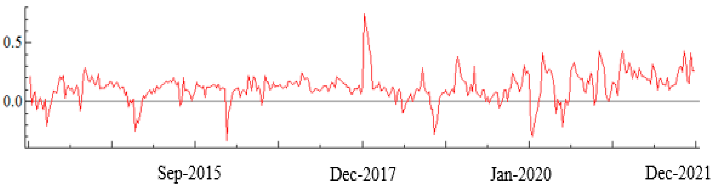
For conditional correlation analyses, we use VAR-DCC-GARCH model. The estimated conditional correlation graphs in VAR-DCC-GARCH between the returns of variables are used in this paper. Therefore, Figure 1, Figure 2 and Figure 3 show the dynamic conditional correlation trend between USD–TEPIX, gold–TEPIX, and USD-gold, respectively.

The dynamic conditional correlation volatility between USD–TEPIX in the range of −0.2657 and 0.7558. The mean correlation coefficient of volatility is 0.1068. These volatilities are positive for most years. Figure 2 shows the dynamic conditional correlation between the returns of gold and TEPIX. The mean correlation coefficient volatility in the period under study is 0.12098. The highest and lowest correlation coefficients between gold–TEPIX are 0.7458 and −0.3338, respectively. 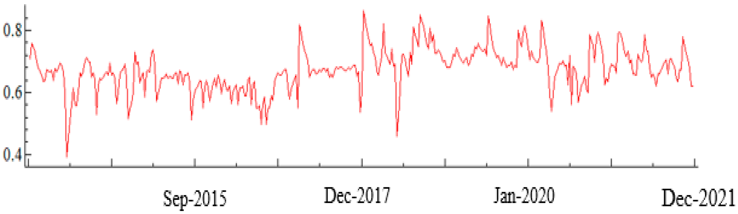Figure 3 shows the dynamic conditional correlation of the returns of USD and gold. The mean correlation coefficient is 0.67409. The highest and the lowest correlation coefficients are 0.8626 and 0.3924, respectively.

The results show that the correlations between gold–TEPIX, USD–TEPIX, and gold–USD are positive. In addition, the correlation between gold–USD is the biggest than the others. It means that investing in the stock market can be considered as an appropriate investment against gold and USD and vice versa. Moreover, these figures show that co-movement between conditional correlations variables exist from early 2018 to December 2021.

3.1. Forecasting Performance

In this section, the wavelet-based random forest is used to select the best model for forecasting. In fact, we compare out-of-sample forecasting of two approaches, VAR-DCC-GARCH and DCC-GARCH, using the wavelet-based random forest (WRF). For this purpose, the time series of volatilities are calculated using the VAR-DCC-GARCH and DCC-GARCH methods, then these volatilities in the financial markets are predicted using the wavelet-based random forest.

Table 6. Model performance metrics.

		VAR-DCC-GARCH				DCC-GARCH
		MSE	RMSE	R-Sq	MAE	MSE	RMSE	R-Sq	MAE
USD	Train	19.40	4.4	0.93	1.8	66.85	8.17	0.88	3.2
	Test	3.4	1.8	0.98	1.16	13.03	3.6	0.97	2.11
gold	Train	10.5	3.2	0.97	1.62	28.61	5.35	0.93	2.44
	Test	3.5	1.87	0.98	1.21	9.46	3.07	0.97	1.96
TEPIX	Train	3.47	1.86	0.89	0.96	22.52	4.74	0.86	2.20
	Test	13.27	3.64	0.95	2.27	50.7	7.07	0.94	3.96

shows the performance metrics of the WRF modeling approach employed in this study. Comparing the RMSE, MSE, R-squared, and MAE, it indicates that the VAR-DCC-GARCH model outperforms the DCC-GARCH model.

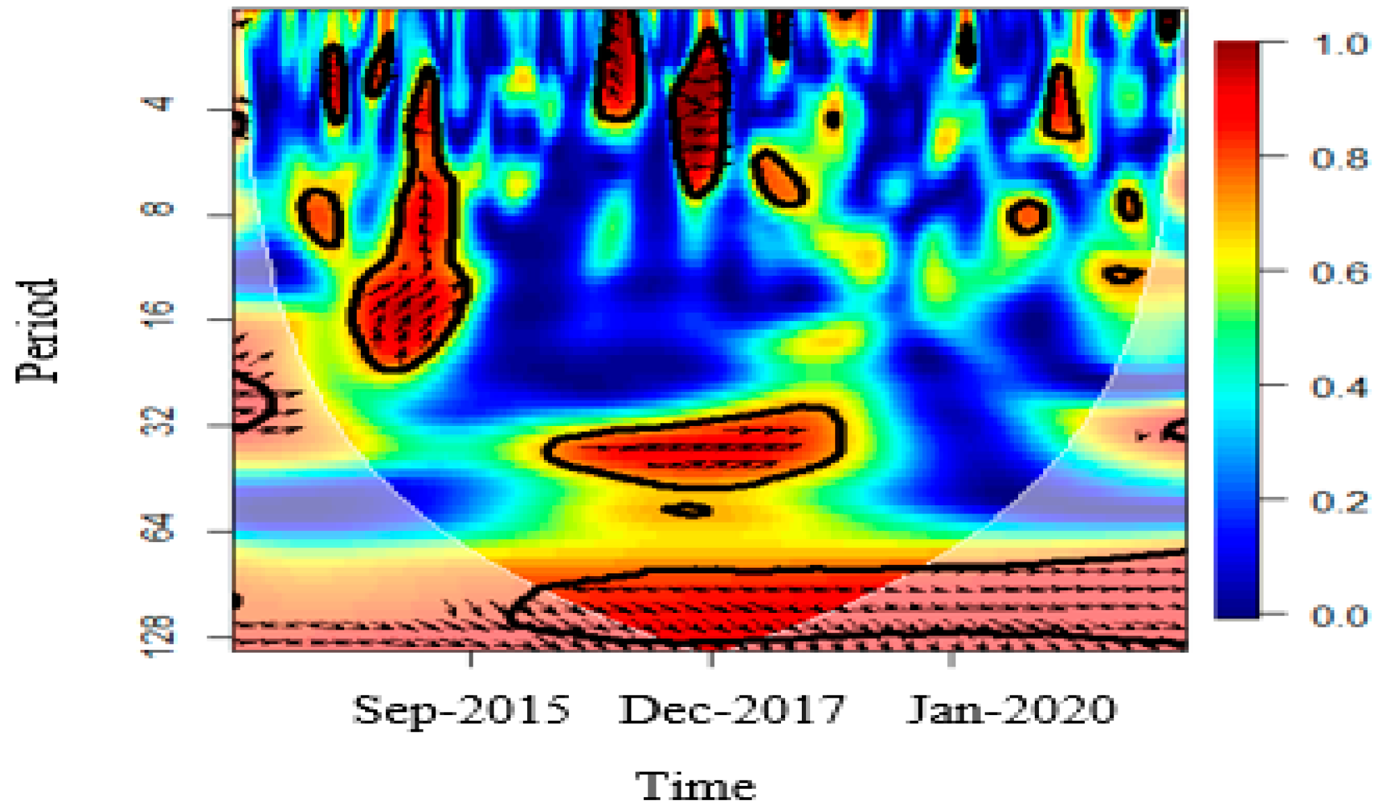
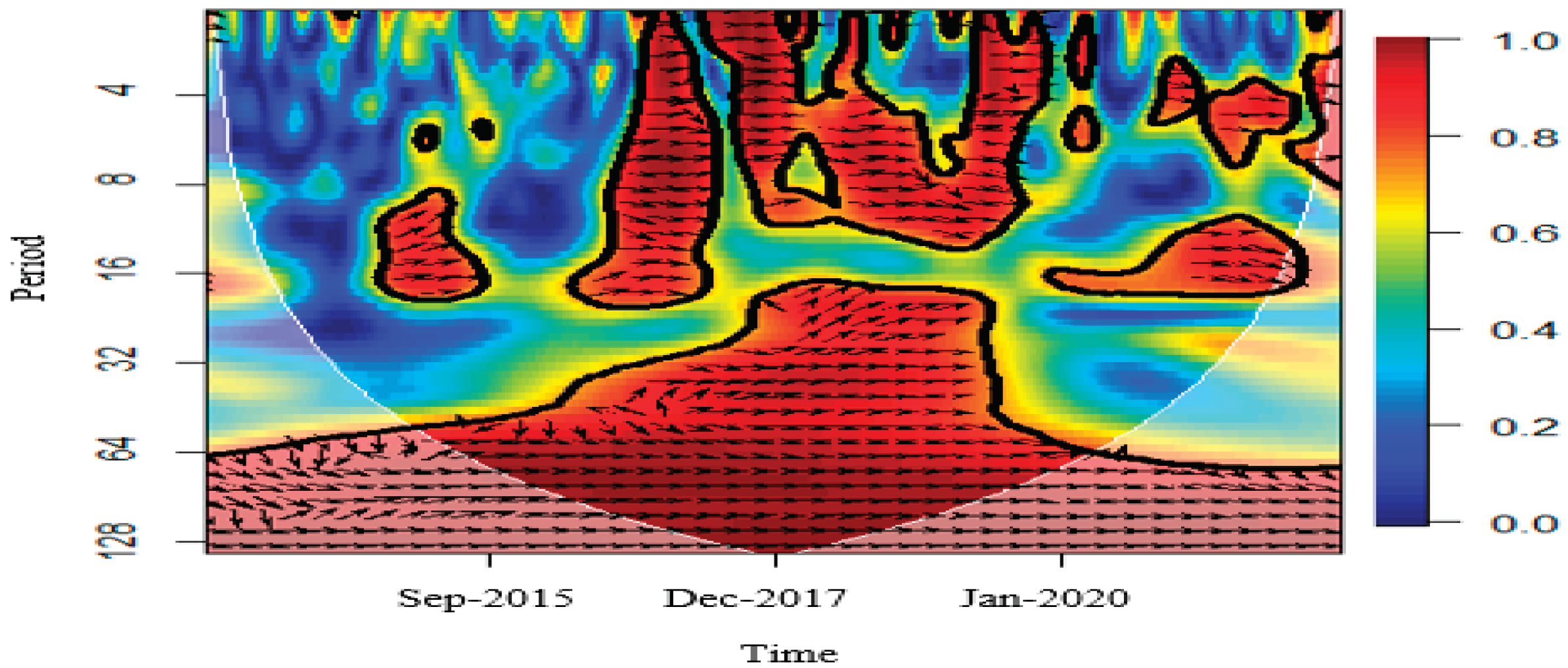
3.2. Results of Wavelet Coherence Estimation

Applying volatilities extracted from VAR-DCC-GARCH model, the wavelet approach is used to examine the interconnected relationships between markets. The results of the coherence estimation are shown in Figure 4, Figure 5 and Figure 6. The color of the graph shows the strength of coherency, ranging from blue (low coherency) to red (high coherency). Therefore, the more the color spectrum trends to red, the higher the correlation. The horizontal axis represents the time scale and the vertical axis represents the frequency. The graphs also show the frequency of the period (short, medium, and long term). In this way, the shortest period is 4 days and the longest is 256 days.

Figure 4 shows the correlation wavelet of volatilities in USD–TEPIX. According to the Figure, the color blue dominates for the most part in the short run, so there is no high correlation in the short run between volatilities in USD–TEPIX. However, in the medium term, despite the orange and red color spectrum between 2014 and 2015, it can be said that the correlation between USD–TEPIX volatilities has increased in the medium term. In the long run, there is correlation from 2016 to 2021.

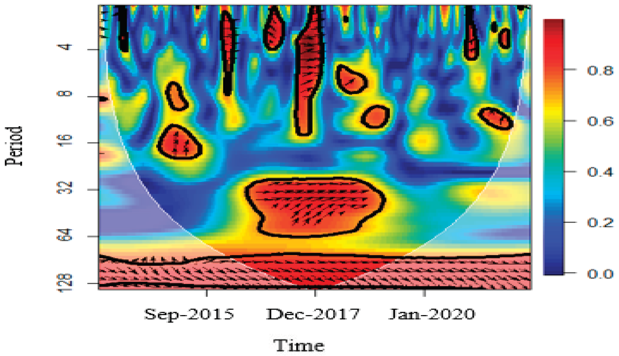
The wavelet correlation analysis in gold–TEPIX volatilities is presented below in Figure 5. In the short run, given that the blue color spectrum is predominant in most of the periods, there is a low correlation between volatilities in the pairs of gold and TEPIX. In the medium term, given the dominance of the orange and yellow spectrum, especially in the period between 2017, there is a correlation between the volatility of the two markets. In the long run, there is correlation between the volatility of these two markets.

Finally, Figure 6 shows the correlation wavelet analysis on USD–gold volatilities. According to this figure, in the short and medium term from early 2016 to January 2020, given the dominant red color spectrum, a high correlation is observed in the volatilities of the returns of gold–USD. In the long run, the correlation trend in the volatilities of gold–USD has been increasing.

4. Conclusions

This study investigated the time-varying co-movement between the volatility of gold, exchange rate, and stock market returns in Iran. To do so, we first modelled the conditional correlations of financial markets using VAR-DCC-GARCH and DCC-GARCH models. Then, we compared the out-of-sample forecasting of these models. Finally, the CWT was used to study the co-movement between financial markets’ volatilities. The results of the wavelet-based random forest model showed that the forecasting performance of VAR-DCC-GARCH model is better than that of DCC-GARCH model. Furthermore, there are positive correlations between the returns of gold–TEPIX and USD–TEPIX, as well as the returns of USD–gold. On the other hand, the correlation between the returns of USD–gold is higher than the other paired markets. This result implies that investors can use stocks as a suitable investment against gold and USD to increase profitability and reduce risk in their portfolio, and vice versa. In addition, the existence of gold and USD in their portfolio can significantly eliminate the benefits of portfolio diversification and increase their portfolio risk. The results of the wavelet analysis showed that the correlation process of the volatilities in the returns of gold–USD is increasing in the medium and long term. This result helps investors to maximize profitability in the short, medium, and long terms by choosing different assets in their portfolios.