Estimation of Suspended Sediment Concentration of Keenjhar Lake through Remote Sensing ^†

Abstract

Water quality is one of the most concerning issues in megacities. Karachi is the world’s third most populated city, with poor water supply and management. The city obtains more than 80 percent of its water from Keenjhar Lake, the second-largest freshwater lake in the country. Keenjhar Lake and all other water bodies currently lack a water quality monitoring system. This study provides a solution to monitor water quality by remote sensing by calculating the lake’s suspended sediment concentration and other quality parameters. To calculate the surface reflectance values, satellite images from Landsat 8 are analyzed in ENVI 5.3 and QGIS 3.10. The reflectance values from different sampling points are compared with spectral signatures to calculate the concentration and validated with several regression equations and standard established relations.

1. Introduction

Water quality is a relatively new study area in Pakistan as the country lacks basic education and a proper monitoring system. Freshwater lakes are a major source of drinking water; therefore, a quality monitoring system is essential to ensure health standards. 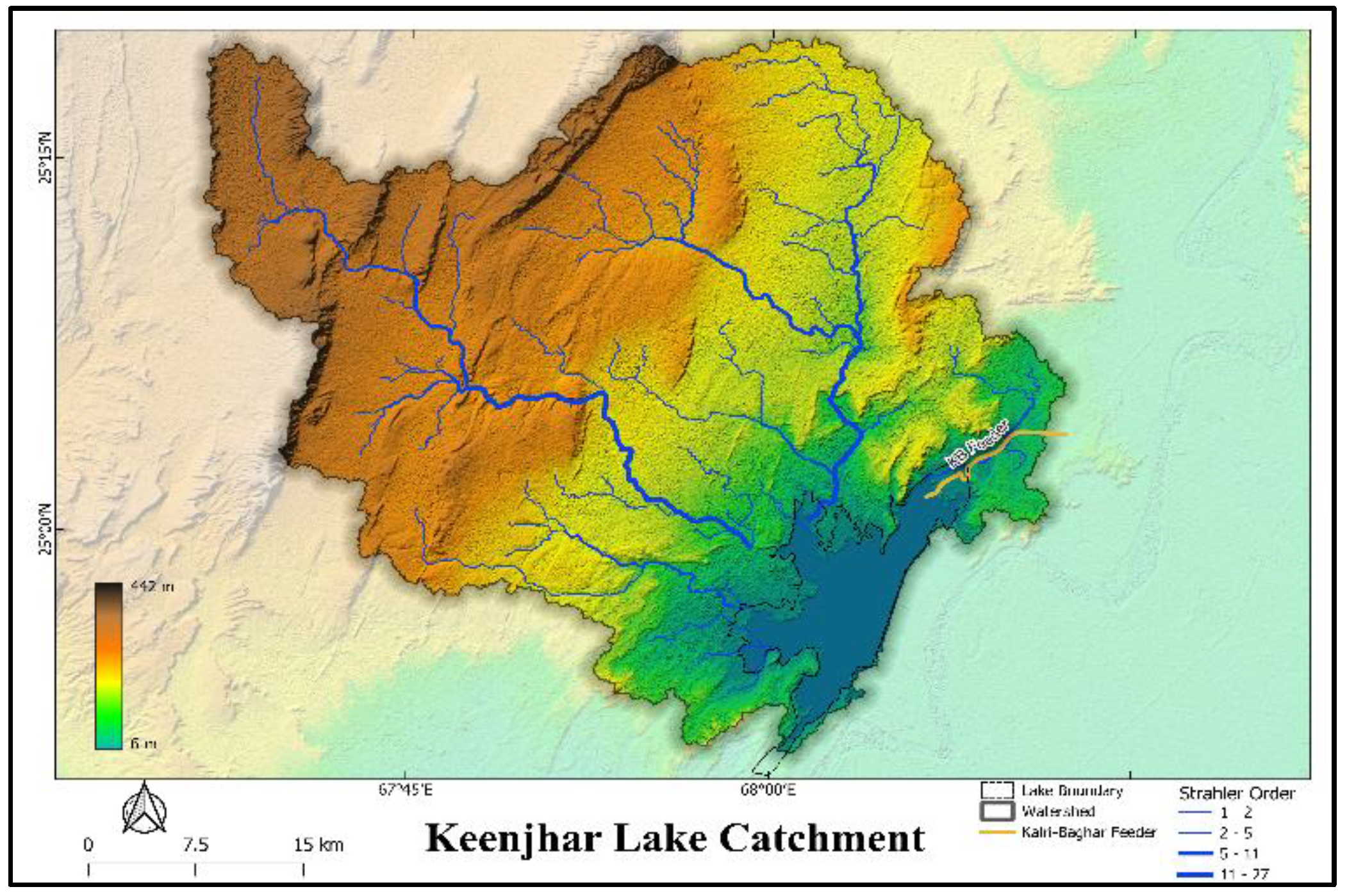Sediment is one of the major sources of pollutants as it carries various polluting elements as well as metals, nitrate, orthophosphate, and carbon and deteriorates the quality of the water body [1]. Major sources of sediment include non-point runoff and the water supply by an unlined canal. The purpose of this study is to use remote sensing techniques to determine suspended sediment concentrations in Keenjhar Lake for water quality monitoring and evaluation. Keenjhar Lake is the largest artificial lake in Pakistan and the major source of water supply to the cities of Karachi and Thatta. It is situated from 67.70° E to 68.00° E and 24.75° N to 25.25° N, with a capacity of roughly 0.5 MAF and a depth of 1 m to 9 m. It has the main recharge source of KB Feeder, and some streams discharge runoff in the monsoon season. The lake is a major source of supply of drinking water in the neighboring cities and towns, and a large number of people visit regularly from Karachi, Hyderabad, and Thatta to enjoy picnics, swimming, fishing, boating, and other recreational activities. When rainwater reaches the lake via the Haroolo drain, it contaminates the water, making it doubtful to drink when mixed with the lake water (SUPARCO). Furthermore, the sediment yield from the unlined Karli Baghar (KB) Canal contributes to degradation of water quality and reduction in the lake’s storage capacity. Figure 1 shows the catchment and drainage pattern of Keenjhar lake while range of quality is shown in

Table 1. A general range of water quality of the lake by tested samples.

Sr. No	Parameter	Range	WHO Standards
1	Temperature, C	30.2–31.8	-
2	pH	7.33–8.12	6.5–8.5
3	Turbidity, NTU	10.5–50	4
4	Conductivity, uS/cm	1937–17,390	400
5	Dissolved Oxygen, (DO), mg/L	11.1–15.8	5–9.5
6	Total Dissolved Solids (TDS), mg/L	1161–4440	1000
7	Hardness, mg/L of CaCO3	450–1425	500
8	Sulfate, mg/L	188–760	400
9	Chloride	515–2255	250
10	Nitrate	0.2–3.5	10

.

Due to the lack of water quality monitoring infrastructure in Pakistan, long-range remote sensing satellite images are employed to determine the water quality parameters. This method is used to compute the suspended sediment concentration (SSC) because sediment plays such a large influence in quality degradation [2,3]. As stated earlier, sediment transports the majority of orthophosphate, nitrate, and pesticides. It also decreases the amount of accessible oxygen in the water and promotes eutrophication by lowering the amount of dissolved oxygen in the water body [3] Overall, it is a solid quality indicator.

2. Methodology

The process includes the acquisition and pre-processing of images, radiometric and atmospheric correction, calculation of surface reflectance values, and transformation of the spectral signatures into water quality parameters. The processing methodology derived from the literature review is comprised of three stages, given below, and shown in Figure 2.

• Minimum value extraction.
• Radiometric correction, including cloud masking.
• Extraction and averaging of surface reflectance values in sampling region of interest (ROI).

The objective of image processing is to calculate reflectance from the image. Everything on Earth has a unique reflectance range of different wavelengths of the electromagnetic spectrum, known as the spectral signature. These signatures change with the change in properties, concentration, type, or nature of the object.

Reflectance can be calculated by,

$$\mathsf{\rho }=\frac{\mathrm{L}}{\mathrm{E}}$$

(1)

where ρ is reflectance, L is outgoing radiance, and E is incidence irradiance (incoming from the Sun).

The outgoing radiance (L) is calculated by radiometric calibration, which means converting the pixel value of the image into a digital number (DN).

$$\mathrm{DN}=\left(\frac{{\mathrm{L}}_{\max }-{\mathrm{L}}_{\min }}{255}\times \mathrm{L}\right)+\mathrm{B}$$

(2)

The incoming irradiance (E) is calculated by solar elevation correction and Earth–Sun distance;

$$\mathrm{E}=\frac{{\mathrm{E}}_{\mathrm{o}}\times \cos \mathsf{\theta } }{{\mathrm{d}}^2}$$

(3)

The radiometric and atmospheric calibration have prepared the necessary input to calculate reflectivity. The path irradiance is subtracted from total irradiance to estimate outgoing radiance, and DN is converted into radiance at the sensor by another set of equations. Several other corrections, such as haze, cloud, and water masking, are performed. The atmospherically corrected reflectance ($\mathsf{\rho }$_λ) is the outcome using the Top of Atmopheric (TOA) reflectance (L_λ) minus the rescaled and corrected DN_min value, correcting for variations in the angle, distance, and brightness of the Sun throughout the year [4].

$${\mathsf{\rho }}_{\mathsf{\lambda }}=\frac{\left[\mathsf{ӆ}{\mathrm{d}}^2\left({\mathrm{L}}_{\mathsf{\lambda }}-{\mathrm{L}}_{\mathrm{haze}}\right)\right]}{\left[{\mathrm{ESUN}}_{\mathsf{\lambda }}\times \mathrm{Cos}\left({\varnothing }_{\mathrm{s}}\frac{\mathsf{ӆ}}{180}\right)\right]}$$

(4)

Landsat 8 image courtesy of the U.S. Geological Survey was chosen for this study since it is one of the most widely used sources for measuring water quality. A Landsat 8 image was acquired and pan-sharpened to a resolution of 15 m. ENVI 5.3 (Exelis Visual Information Solutions, Boulder, CO, USA) was used for the preprocessing and correction of images. There are some bands that water absorbs completely, and some are reflected all the way. The combination of these bands, along with the bands that favor the type of impurity, is usually used in any study of this scope. Most water quality examinations employ the visible and near-infrared (NIR) regions of the electromagnetic spectrum, so specific bands are used for the assessment after the preprocessing of the images.

2.1. Value Extraction

After the preprocessing of images, each pixel value is transformed into a Digital Number (DN). Now, using the photographs, find the DN value that is the lowest. This value is kept constant so that lakes and related sample events from the same Landsat image have the same DN minimum value [4]. After the DN_min value has been recovered, the images are clipped to the rectangular area of the lake because water levels fluctuate and cutting intricate lake boundary vectors is time-consuming [4].

2.2. Radiometric and Atmospheric Correction

Satellite remote sensing systems such as DOS can detect atmospheric and radioactive adjustments. By shifting histograms, the dark object subtraction (DOS) method adjusts for additive radiometric inaccuracy. The DOS correction from atmospheric particles can account for scattering, refraction, and absorption of light [4]. The solar zenith angle and distance between Earth and the Sun, which are automatically extracted from the image header file (metadata), as well as the scene’s pixel values, are recalculated to the top of atmosphere (TOA) values initially collected by the sensor using Equation (5) [4].

$${\mathrm{L}}_{\mathsf{\lambda }}={\mathrm{M}}_{\mathsf{\rho }}\times \mathrm{QCAL}+{\mathrm{A}}_{\mathsf{\rho }}$$

(5)

where L_λ represents TOA reflectance, QCAL represents quantized calibrated pixel values in DN, M_ρ represents multiplicative rescaling, and A_ρ represents additive scaling [4].

Equation (5) transforms to TOA reflectance without considering atmospheric effects. DOS calculates rescaling factors based on the lowest and highest calibration values, which include DOS correction and Sun angle adjustment. The general and extended variants of this equation are explained in Equations (6) and (7):

$${\mathrm{L}}_{\mathrm{haze}}={\mathrm{HL}}_{\min }-{\mathrm{L}}_{1\%}$$

(6)

$${\mathrm{L}}_{1\%}=\frac{\left[0.01+{\mathrm{ESUN}}_{\mathsf{\lambda }}\times \mathrm{Cos}{\left({\varnothing }_{\mathrm{s}}\frac{\mathsf{ӆ}}{180}\right)}^2\right]}{\left(\frac{\mathsf{ӆ}}{{\mathrm{d}}^2}\right)}$$

(7)

The majority of the input data for Equations (5)–(7) may be found in the Landsat metadata (.MTL) file that comes with the picture when downloaded from the USGS site. One of the known parameters supplied for each satellite is the solar zenith angle in degrees, which is calculated from the Sun elevation contained in the metadata minus 90. The rescaled and corrected DN_min value L_haze is utilized to correct the rescaled image values during the correction procedure (Equation (4)).

By subtracting the TOA reflectance (L) from the rescaled and adjusted DN_min value, which accounts for variations in the Sun’s angle, distance, and brightness during the year, the atmospherically corrected reflectance ρ is computed [4]. Use Equation (1) to convert values to spectral radiation, then Equation (2) to convert spectral radiance to surface temperature to radiometrically correct the thermal band (6) [4]. Different band combinations utilized to detect the suspended silt are shown in the figure below, where sediment can be identified in different bright colors as shown in Figure 3.

2.3. Data Extraction

Pixels of the x–y position of the in-situ sample point were chosen to analyze the reflectance data. The pixel window size was chosen based on the idea that the quality characteristics of water are heterogeneous and fluctuate regularly due to seasonal, solar, and meteorological effects; therefore, a larger window will capture some of that fluctuation [5]. The images in the Figure 3 express different band compositions, calibrated and processed before being used to determine reflectance in six different locations. The subset images focusing the study area of the lake shown in Figure 4. In this case, selection of date and time as well pixel locations were dictated by official and confidential water quality sample tested data (which cannot be shown here) in the same location.

All of this processing was completed in ENVI 5.3, and the results were cross-checked by Semi-Automatic Classification (SCP) in QGIS 3.10 (QGIS Development Team, 2021. QGIS Geographic Information System. Open Source Geospatial Foundation).

3. Results

The image shown in Figure 5 represents the percentage reflectance values of different sampling locations in different wavelength regions. Each reflectance curve corresponds to a certain sediment concentration.

The map in Figure 6 demonstrates the spatially distributed suspended sediment concentration of different regions of interest in the lake corresponding to the percentage reflectance for various regions of the wavelength of the reflected light shown in Figure 5.

Although the results were validated from the samples’ data, the data were not allowed to be published due to the confidentiality of the report. Moreover, the open-source SSC data for the lake were unavailable. Hence, the results were calibrated and validated with the help of previous studies using the established and tested relationships of SSC and reflectance for the estimation of concentration values. The suspended sediment concentration for different surface reflectance values in different ranges of spectrum wavelengths was calculated and compared by at least five different established relations. Jerry C. Ritchie [3] established a relationship between the wavelength of the light reflected and the percentage reflectance for various SSC as shown in Figure 7.

Ritchie [3] also compiled several relationships between SSC and wavelengths from the literature shown in Figure 8. Some of these equations were used for calibration and validation.

The map in Figure 6 correlates with the drainage pattern of the study area presented in Figure 1. The highest SSC is at the KB Feeder inlet, an unlined canal-feeding the lake that is the most dominant source of sediment in the lake. Runoff does not play a major part in sediment delivery to the lake due to the presence of protection wall along the major portion of the western boundary of the lake.

4. Conclusions

Water quality monitoring is an absolute health standard to maintain. This study aimed to estimate a very important quality parameter, i.e., suspended sediment concentration, with the help of remote sensing and imagery analysis. Landsat 8 images were acquired and analyzed by ENVI 5.3, and QGIS 3.10. The images were radiometrically and atmospherically corrected to calculate the surface reflectance and obtain the spectral signature. These reflectance values were compared with established relationships between surface reflectance and SSC to estimate the SSC values of the lake. The results show that the SSC of the lake ranges from 398 mg/L to 48 mg/L, which is in the range per WHO water quality standards. The study demonstrated the remote sensing technique to be an efficient and sustainable method to monitor the long-term water quality of any water body. Further research can be conducted to calibrate and establish a more accurate relationship between surface reflectance and SSC for Keenjhar Lake. This can help in monitoring the water quality at least twice or sometime thrice a month when Landsat images are available for the lake.