
Indoor Position Estimation Using Ultrasonic Beacon Sensors and Extended Kalman Filter †


Abstract
:1. Introduction
2. Position Estimation Algorithm
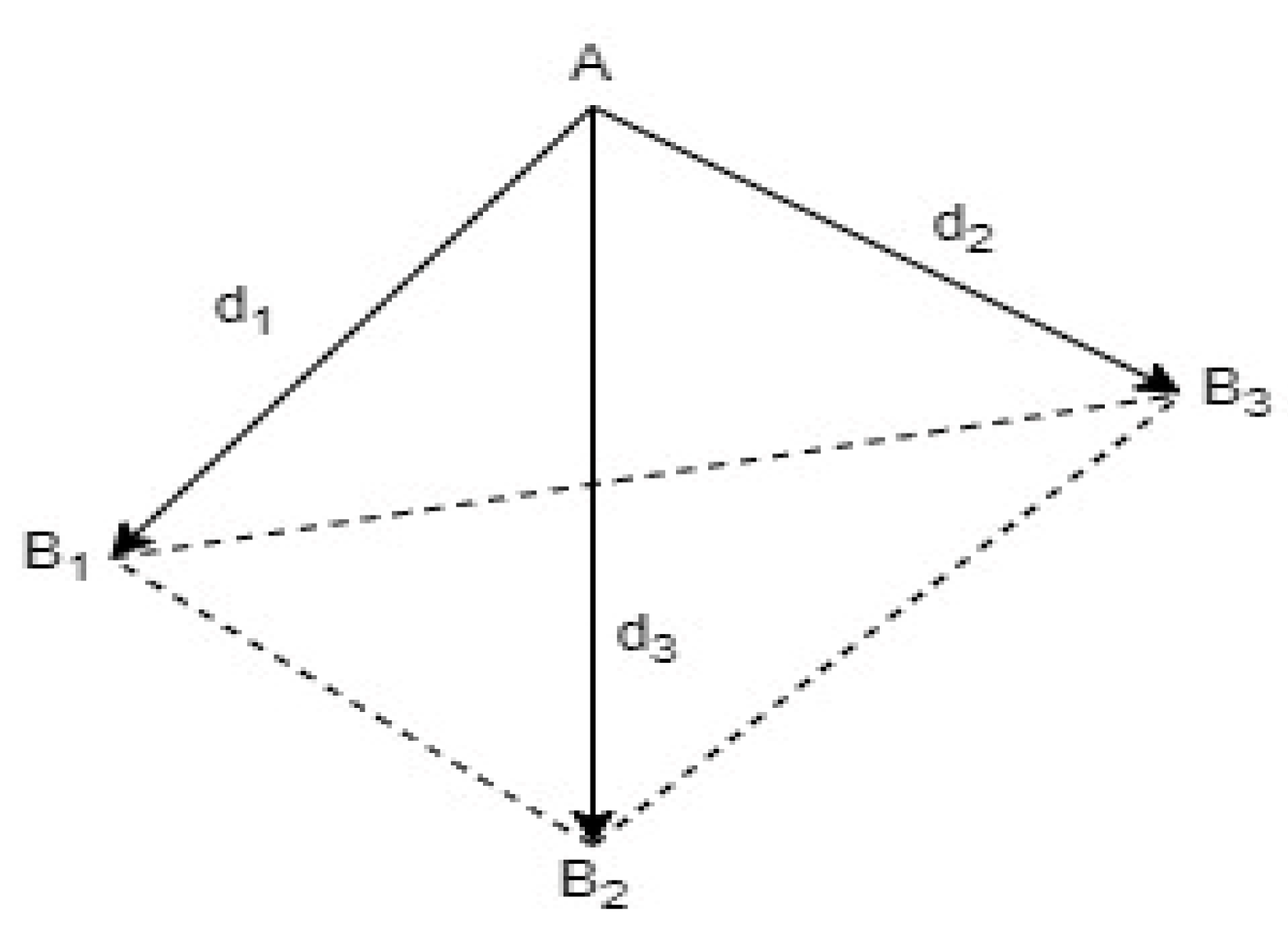
2.1. Geometric Approach
2.2. Sensor Fusion Algorithm
3. Simulation System and Results
4. Conclusions
Author Contributions
Funding
Institutional Review Board Statement
Informed Consent Statement
Data Availability Statement
Conflicts of Interest
References
- Valavanis, K.P.; Vachtsevanos, G.J. UAV Applications: Introduction; Springer: Amsterdam, The Netherlands, 2015. [Google Scholar]
- Samad, T.; Bay, J.S.; Godbole, D. Network-centric systems for military operations in urban Terrain: The role of UAVs. Proc. IEEE 2007, 95, 92–107. [Google Scholar] [CrossRef]
- Li, Z.; Liu, Y.; Walker, R.; Hayward, R.; Zhang, J. Towards automatic power line detection for a UAV surveillance system using pulse coupled neural filter and an improved Hough transform. Mach. Vis. Appl. 2010, 21, 677–686. [Google Scholar] [CrossRef] [Green Version]
- Nirjon, S.; Liu, J.; DeJean, G.; Priyantha, B.; Jin, Y.; Hart, T. COIN-GPS: Indoor localization from direct GPS receiving. In Proceedings of the 12th Annual International Conference on Mobile Systems, Applications, and Services—MobiSys 2014, Bretton Woods, NH, USA, 16–19 June 2014; pp. 301–314. [Google Scholar]
- Vasisht, D.; Kumar, S.; Katabi, D. Decimeter-Level Localization with a Single WiFi Access Point. In Proceedings of the USENINX Symposium on Networked Systems Design and Implementation, Santa Clara, CA, USA, 16–18 March 2016; pp. 165–178. [Google Scholar]
- Zafari, F.; Papapanagiotou, I.; Christidis, K. Microlocation for internet-of-things-equipped smart buildings. IEEE Internet Things J. 2016, 3, 96–112. [Google Scholar] [CrossRef] [Green Version]
- Mur-Artal, R.; Tardos, J.D. ORB-SLAM2: An open-source SLAM system for monocular, stereo, and RGB-D cameras. IEEE Trans. Robot. 2017, 33, 1255–1262. [Google Scholar] [CrossRef] [Green Version]
- Forster, C.; Pizzoli, M.; Scaramuzza, D. SVO: Fast semi-direct monocular visual odometry. In Proceedings of the 2014 IEEE International Conference on Robotics and Automation (ICRA), Hong Kong, China, 31 May–7 June 2014; pp. 15–22. [Google Scholar]
- Engel, J.; Koltun, V.; Cremers, D. Direct sparse odometry. IEEE Trans. Pattern Anal. Mach. Intell. 2018, 40, 611–625. [Google Scholar] [CrossRef] [PubMed]
- Grisetti, G.; Stachniss, C.; Burgard, W. Improved techniques for grid mapping with rao-blackwellized particle filters. IEEE Trans. Robot. 2007, 23, 34–46. [Google Scholar] [CrossRef] [Green Version]
- Kohlbrecher, S.; von Stryk, O.; Meyer, J.; Klingauf, U. A flexible and scalable SLAM system with full 3D motion estimation. In Proceedings of the 2011 IEEE International Symposium on Safety, Security, and Rescue Robotics, Kyoto, Japan, 1–5 November 2011; pp. 155–160. [Google Scholar]
- Ren, R.; Fu, H.; Wu, M. Large-scale outdoor SLAM based on 2D lidar. Electronics 2019, 8, 613. [Google Scholar] [CrossRef] [Green Version]
- Chintalapudi, K.; Padmanabha Iyer, A.; Padmanabhan, V.N. Indoor localization without the pain. In Proceedings of the Annual International Conference on Mobile Computing and Networking, Mobicom, Chicago, IL, USA, 20–24 September 2010; pp. 173–184. [Google Scholar]
- Gomez, C.; Oller, J.; Paradells, J. Overview and evaluation of bluetooth low energy: An emerging low-power wireless technology. Sensors 2012, 12, 11734–11753. [Google Scholar] [CrossRef] [Green Version]
- Wang, Y.; Ye, Q.; Cheng, J.; Wang, L. RSSI-Based Bluetooth Indoor Localization. In Proceedings of the 11th International Conference on Mobile Ad-Hoc and Sensor Networks, MSN 2015, Shenzhen, China, 16–18 December 2015; pp. 165–171. [Google Scholar]
- Cabarkapa, D.; Grujic, I.; Pavlović, P. Comparative analysis of the Bluetooth Low-Energy indoor positioning systems. In Proceedings of the 2015 12th International Conference on Telecommunication in Modern Satellite, Cable and Broadcasting Services (TELSIKS), Nis, Serbia, 14–17 October 2015; pp. 76–79. [Google Scholar]
- Rida, M.E.; Liu, F.; Jadi, Y.; Algawhari, A.A.; Askourih, A. Indoor location position based on bluetooth signal strength. In Proceedings of the 2015 2nd International Conference on Information Science and Control Engineering, ICISCE 2015, Shanghai, China, 24–26 April 2015; pp. 769–773. [Google Scholar]
- Kriz, P.; Maly, F.; Kozel, T. Improving Indoor Localization Using Bluetooth Low Energy Beacons. Mob. Inf. Syst. 2016, 2016, 2083094. [Google Scholar] [CrossRef] [Green Version]
- Aiello, G.R.; Rogerson, G.D. Ultra-wideband wireless systems. IEEE Microw. Mag. 2003, 4, 36–47. [Google Scholar] [CrossRef]
- Chehri, A.; Fortier, P.; Tardif, P.M. UWB-based sensor networks for localization in mining environments. Ad Hoc Netw. 2009, 7, 987–1000. [Google Scholar] [CrossRef]
- Norrdine, A. An Algebraic Solution to the Multilateration Problem. In Proceedings of the 2012 International Conference on Indoor Positioning and Indoor Navigation, Sydney, Australia, 13–15 November 2012; pp. 1–4. [Google Scholar]


| Trajectory Name | Beacon Number | Trajectories |
|---|---|---|
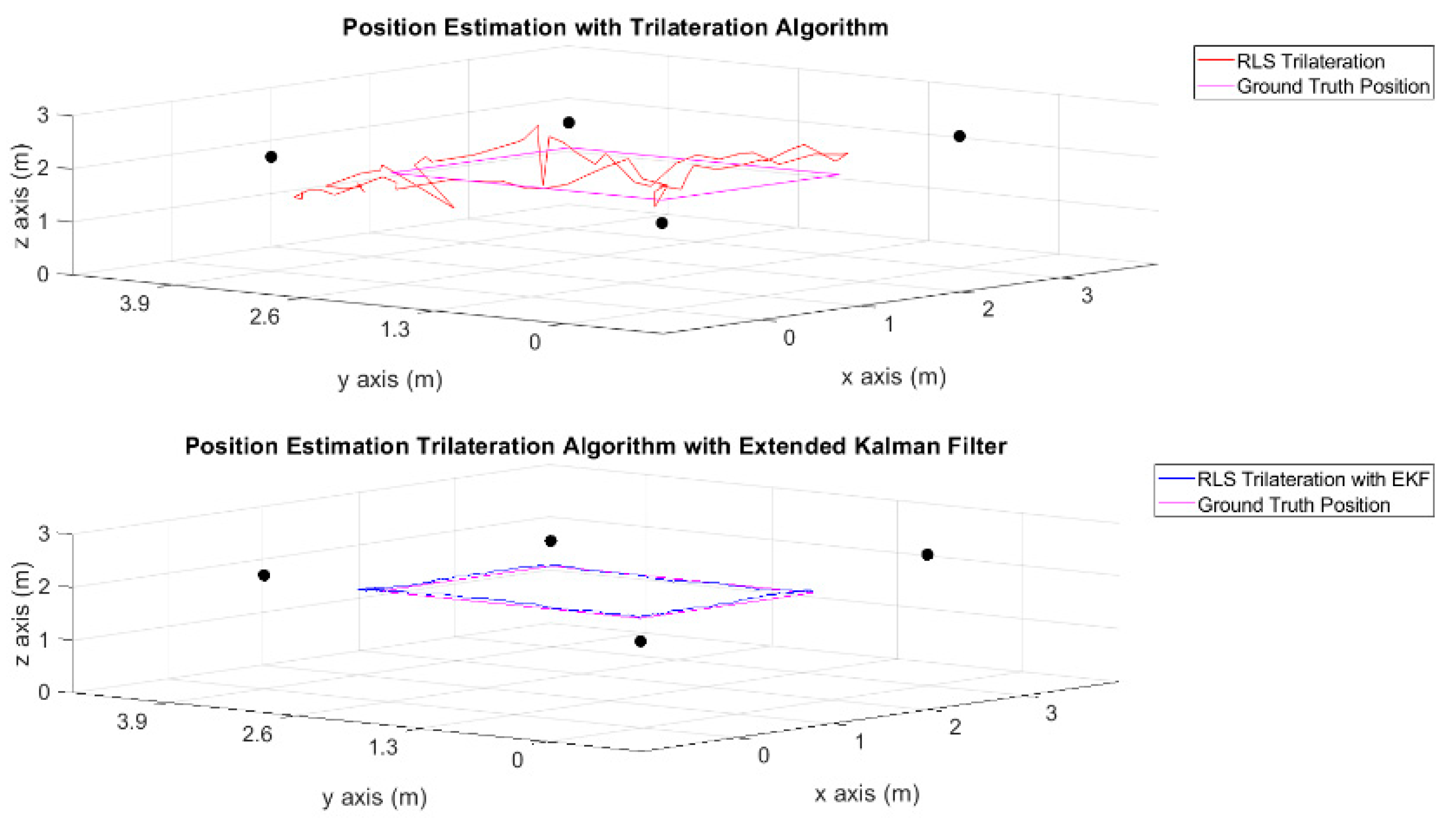
| Trajectory 1 | 5 |  |
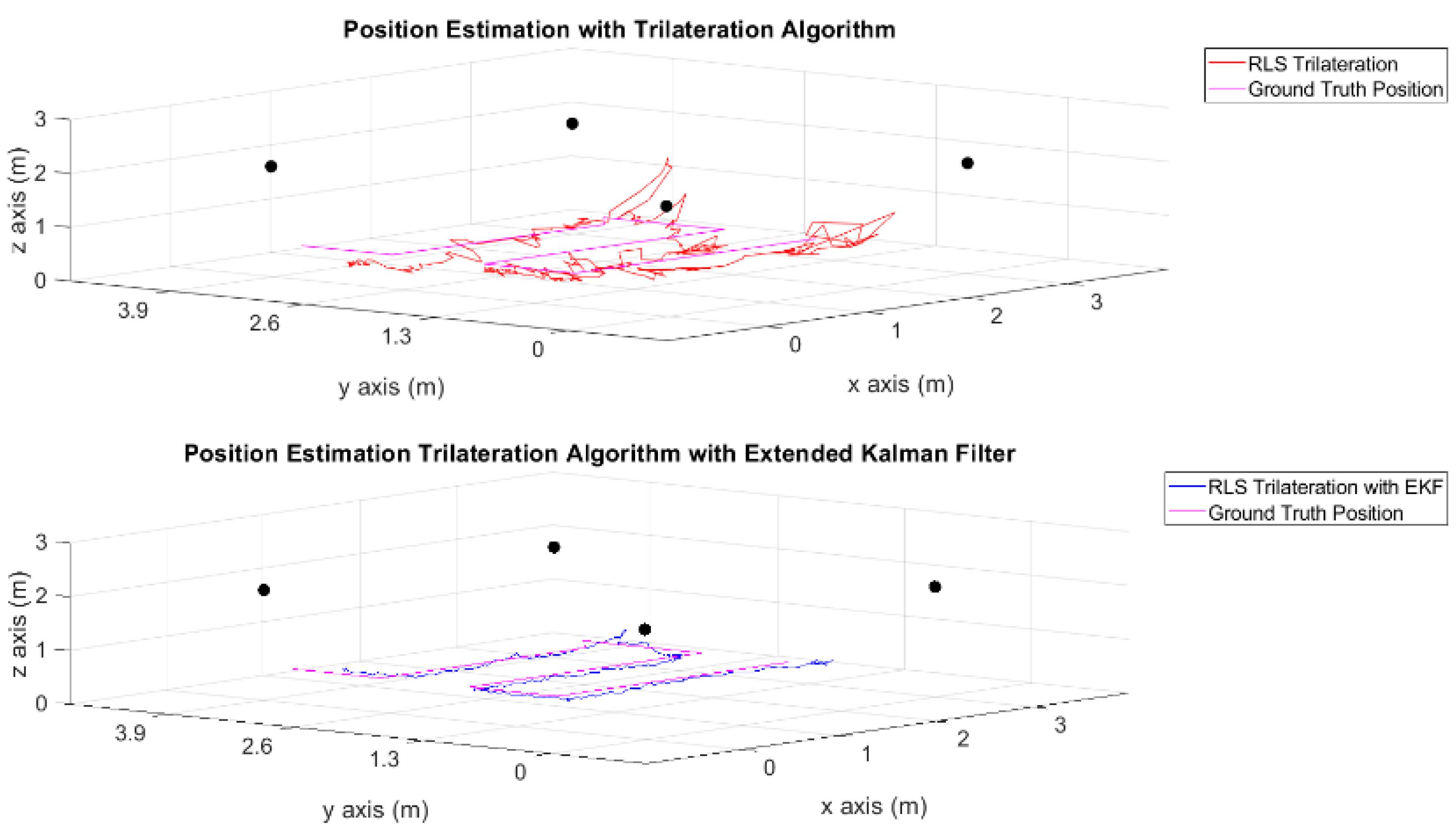
| Trajectory 2 | 5 |  |
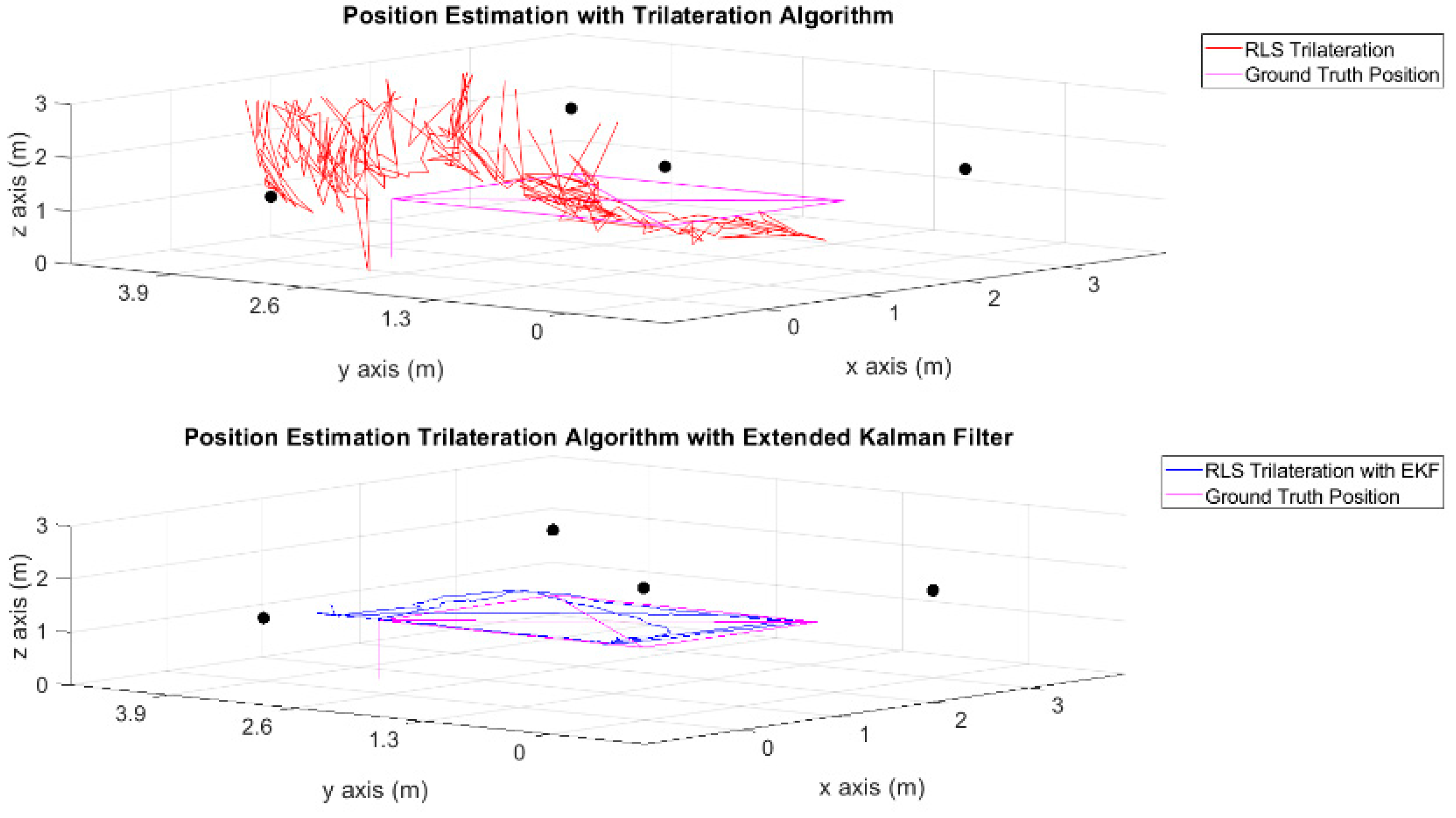
| Trajectory 3 | 5 |  |
| Trajectory | Algorithm | Min Error (m) | Mean Error (m) | Max Error (m) |
|---|---|---|---|---|
| Trajectory 1 | Trilateration Algorithm | 0.073409 | 0.335606 | 0.994064 |
| Trajectory 1 | Trilateration Algorithm + EKF | 0.019016 | 0.061539 | 0.143751 |
| Trajectory 2 | Trilateration Algorithm | 0.077657 | 0.453345 | 1.768042 |
| Trajectory 2 | Trilateration Algorithm + EKF | 0.016976 | 0.082958 | 0.168863 |
| Trajectory 3 | Trilateration Algorithm | 0.353665 | 1.258376 | 5.003108 |
| Trajectory 3 | Trilateration Algorithm + EKF | 0.001041 | 0.083402 | 0.164720 |
Publisher’s Note: MDPI stays neutral with regard to jurisdictional claims in published maps and institutional affiliations. |
© 2022 by the authors. Licensee MDPI, Basel, Switzerland. This article is an open access article distributed under the terms and conditions of the Creative Commons Attribution (CC BY) license (https://creativecommons.org/licenses/by/4.0/).
Share and Cite
Bodrumlu, T.; Caliskan, F. Indoor Position Estimation Using Ultrasonic Beacon Sensors and Extended Kalman Filter. Eng. Proc. 2022, 27, 16. https://doi.org/10.3390/ecsa-9-13353
Bodrumlu T, Caliskan F. Indoor Position Estimation Using Ultrasonic Beacon Sensors and Extended Kalman Filter. Engineering Proceedings. 2022; 27(1):16. https://doi.org/10.3390/ecsa-9-13353
Chicago/Turabian StyleBodrumlu, Tolga, and Fikret Caliskan. 2022. "Indoor Position Estimation Using Ultrasonic Beacon Sensors and Extended Kalman Filter" Engineering Proceedings 27, no. 1: 16. https://doi.org/10.3390/ecsa-9-13353