Finite Element Simulation for Predicting the Magnetic Flux Density for Electromagnetic Vibration Energy Harvester ^†

Abstract

The current revolution in the field of electromagnetic vibration energy harvester requires that both wireless sensor nodes and relevant power sources be cost- and size-optimized while ensuring that, during design/fabrication of the sensor’s power sources, the power deliverable to the sensors be maximum. Flux density dependency on the nature of the magnetic coupling material of VEH magnet-coil transducer is well reported while reports on size-optimized but improved performance in the VEH is available. This paper presents on the realization of an approach to ensure an accurate prediction of size-optimized but maximum power output on the electromagnetic transducer of a VEH. The adopted approach justifiably verifies the geometrically determined flux density on a Finite Element Magnetic Method Software (FEMM) on the permanent magnet (NdFeB N52) as a basis for optimization. An empirical formula—which predicts size-optimized flux density and could be used to predict the performance of a miniature energy harvester for wireless sensor nodes application—was formulated. For the geometry presented in this work, where $l_c$ and $N_{c-2}$ are the effective length and turns on the reference coil, the magnetic flux density, coupling coefficients, coil width and transducer thickness were predicted to optimize at 0.4373 T, 0.3978${\mathsf{\mu }}_3{l}_c{N}_{c-2}$ Tmm, 4.00 mm and 18.40 mm, respectively, with all corresponding to instances when the flux density per unit volume on the coil was approximately 0.4373$/\left({\mathsf{\mu }}_3{\overline{v}}_{c-2}\right)$T${\mathrm{mm}}^{-3}$. The above optimized values were measured on magnet-coil geometry with the smallest overall thickness. However, in comparison to other models, the coil thickness in the optimized geometry was not the least.

1. Introduction

A VEH has proven worthy of having the capacity to sustainably supply electrical power to wireless sensor nodes (WSNs) and body sensor networks (bodyNETs) [1] by scavenging ambient vibrational energy and converting it into useful electrical energy. The scope of scavenging environmental energy has recently attracted interest because it opens a pathway to realizing the sustainable development goals of cutting down carbon footprints that are mostly produced as waste product during energy generation. Previous work concluded structural and electrical based optimization of the energy harvester [2]. An innovative approach on the two-degree-of-freedom (2DOF) linear vibration energy harvester for train application and optimization was analyzed on Multiphysics using the result from numerical magnetic field simulation [3]. The model prototype was fabricated and found consistent with the obtained theoretical results. A study on dynamic responses in 2DOF systems, based on different electrical coil connection and geometry to ascertain which connection mode gives an optimum performance, concluded that series connection is the best in terms of harvested voltage/power, operational bandwidth and normalized power [4]. A path to achieving power maximization on a size optimized/miniature A-battery sized VEH design was reported [5]. The author coupled a non-magnetic (tungsten) inertial mass alongside the axially oriented oscillating magnet to compensate for resonance due to miniaturization. Refs. [6,7] reported a ring-shaped, coil–magnet transducer architecture of VEH with Halbach configuration where a linear Halbach array concentrates its magnetic field in the inner space of the mechanism where a vertically centered single coil was located to increase the resonant mass within a fixed dimension of the transducer. In a separate attempt, the level of the flux density in the power line was measured using an FEMM software during fabrication of the indoor power line based magnetic field energy harvester [8]. In a similar endeavor, measuring the flux density using FEMM on a Halbach array was mentioned in [7].

Without a loss of generality, this paper focuses on realizing an approach to ensure an accurate prediction of the optimum overall size that will maximize the coupling coefficient and power output on the electromagnetic transducer of a VEH.

2. Harvesters Governing Equation

A vibration energy harvester is a device that scavenges and transforms ambient vibration into useable electrical energy that can power sensor nodes. The VEH comprises a coil placed in the field of a permanent magnet such that, during vibration, the coil that is fixed to the free end of a fixed-free mechanical structure will freely oscillate. As much as engineers have keen interest in realizing the above objectives, cost and size optimization remain a valuable pearl held in high esteem during fabrication/design. This work presents a finite element simulation approach to realize size optimization based on the level of the magnetic flux density/coupling in the iron–magnet–coil part of an electromagnetic vibration energy harvester. The focus in this work will be to optimize the iron–magnet–coil geometry with the view to realize more compact, lightweight and cost-effective iron–magnet–coil designs. The general geometry employed to fully characterize the transduction iron–magnet–coil, which will be modeled in the FEMM software, is shown in Figure 1.

From Figure 1, $h_c, h_s$, $h_{\mathrm{a}}$ and $h_{\mathrm{m}}$ are the respective heights of coil, pure iron plate which prevent flux leakages, separation distance between coil and magnets and outer magnet while $w_c,$ $w_s,$ $w_{\mathrm{a}}$ and $w_{\mathrm{m}}$ are the respective widths/thicknesses of the materials earlier mentioned. Equation (1) gives an expression for computing the terms $h_c$ and $h_s$.

$$h_c=h_s=2h_{\mathrm{m}}+h_a$$

(1)

The sufficient clearance between the coil and the magnet, $w_a$, was fixed to 1.5 mm to prevent contact during excitation. The total width of the iron–magnet–coil obtained from Figure 1 is shown in Equation (2).

$$w_T=2\left(w_s+w_{\mathrm{m}}+w_a\right)+w_c$$

(2)

When the geometry is visualized on a 3D plane, the model protrudes by a fixed length $L$ into the page. During excitation, the magnetic flux of the permanent magnet couples into the freely oscillating coil, hence, voltages are induced in the coil according to the principle of electromagnetic induction. $K$ is defined as the degree of coupling that was obtained [9].

$$K=NB{l}_c{c}_f$$

(3)

where $N, B, l_c$ and $c_f$ are effective turn, flux density, effective length and coil fill factor. If none of the magnetic flux couples into the coil, an approximately zero voltage is induced in the coil. Therefore, the coil materials are carefully selected (copper in this case) to ensure that the highest possible degree of coupling is realized. The selected copper wire material is wound into N turns on a nonconductive circular brace to achieve a total coil width/thickness $w_c$.

The Maxwell theory reported divergence and the curl of the flux density where $B=\mu H,$ $E={\epsilon }_{0}D$, $J , D, B, E$ and $H$ are the current density, displacement field, magnetic field, electric field and magnetizing field. μ is the permeability of the magnetic material.

$$\nabla .\left(\mu H\right)=0$$

(4)

$$\nabla \times \left(\mu H\right)={\mu }_{0}J+\frac{1}{c^2}\frac{\partial E}{\partial t}$$

(5)

The physical meaning of Equations (4) and (5) asserts that, for any magnetic system/magnet, there are no isolated magnetic poles, and circulating magnetic fields are produced by changing electric currents. In the eventuality of using more than one magnet, Equation (4) sets an order for which the transduction magnet must be aligned to allow for continuous flux linkage between the several magnets in such a manner that no pole is isolated. In the region of no charge, $J , D$ and $E$ are all equal to zero in Equations (4) and (5). Therefore, the equations predicted a non-changing flux value since no external source of electric charge is in the system.

3. Iron–Magnet–Coil Simulation and Coupling Equations

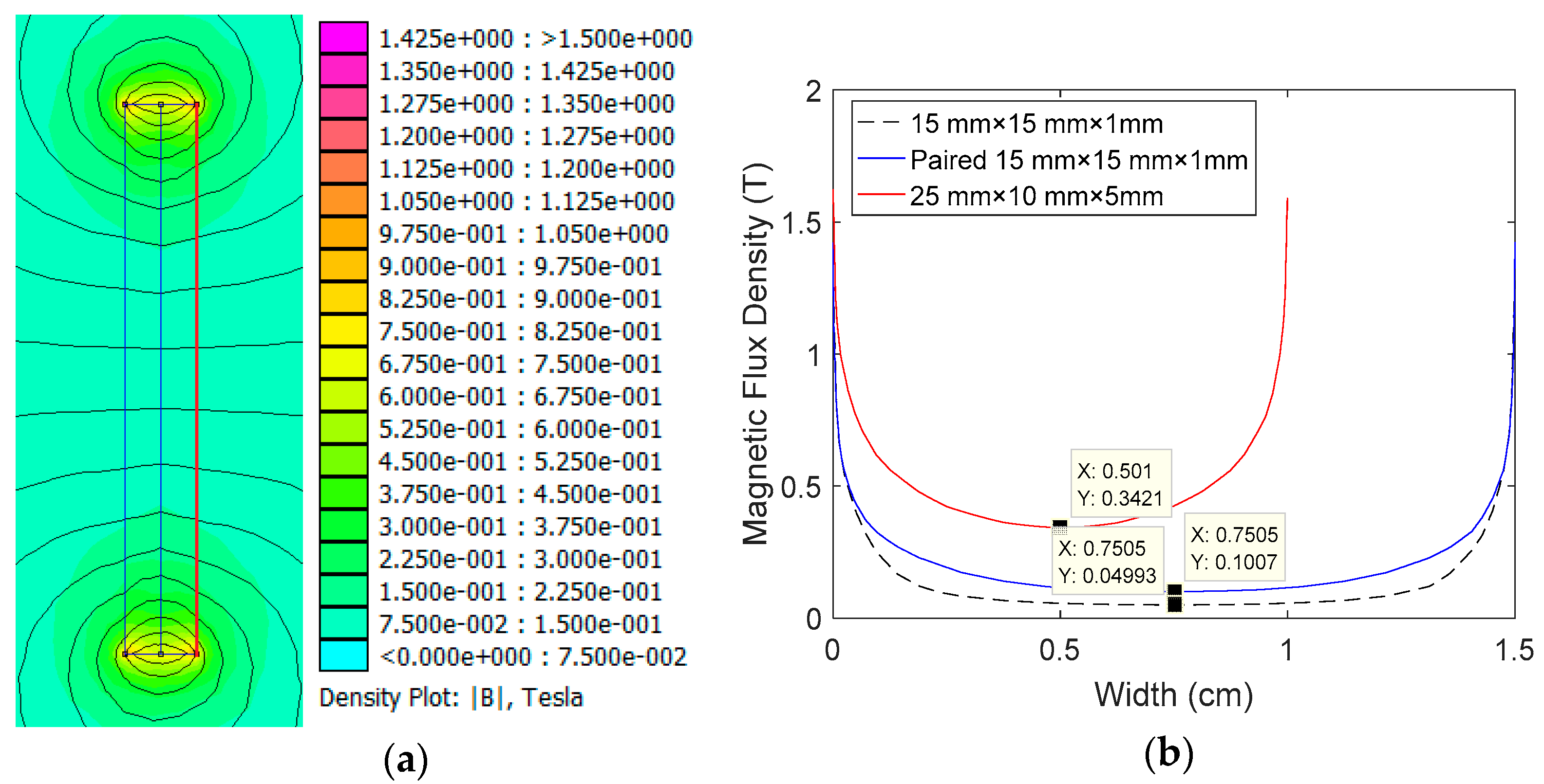
Before the flux density was simulated on FEMM, an initial approach was taken to characterize the flux on a $5 \mathrm{mm}\times 10 \mathrm{mm}\times 25 \mathrm{mm}$ magnet using a Gauss meter actualized to a value of 0.3322 T. However, the FEMM software predicted an average magnet flux density of 0.3421 T, which is also measured on the surface center in Figure 2a, and the flux density across the red line is shown in Figure 2b. This measured value diverges from empirical value to about 4.73 %; however, the level of divergence is considered sufficiently accurate while Figure 2b shows that higher flux occurs at the edges of the magnets.

During FEMM simulation of the coil–magnet model, a total of eight (8) magnets of $15 \mathrm{mm}\times 15 \mathrm{mm}\times 1 \mathrm{mm}$ were paired into four (4) groups as shown in Figure 1 and according to Equation (2). FEMM, however, predicted average magnetic flux density of 0.04993 T and 0.1007 T at the center of the single and paired magnets, respectively, as shown in Figure 2b, while Figure 2a shows the FEMM pattern on the paired magnet.

Adequate flux/coupling prediction requires insight about the distribution of the flux fields in the coils (i.e., flux density per unit volume ($\beta$)). The predicted B values were found consistent with the magnet dimension realizing a $\beta$ value of$2.74\times {10}^{-4} {\mathrm{Tmm}}^{-3}$, 2.234 × ${10}^{-4} {\mathrm{Tmm}}^{-3}$ and $2.219\times {10}^{-4} {\mathrm{Tmm}}^{-3}$ on the $25 \mathrm{mm}\times 10 \mathrm{mm}\times 5 \mathrm{mm}$ and $15 \mathrm{mm}\times 15 \mathrm{mm}\times 1 \mathrm{mm}$ paired and $15 \mathrm{mm}\times 15 \mathrm{mm}\times 1 \mathrm{mm}$ single magnet configurations, respectively. From the above, the magnetic flux density on any NdFeB N52 permanent magnet of known volume $\left(v\right)$ was obtained as

$$B=\beta v$$

(6)

where $\beta$ is the magnetic flux density per unit volume. It was obtained as the ratio of the magnetic flux density associated with each magnet geometry on the FEMM to its volume.

Considering the transducer geometry, a need arose to normalize $v$ and $\beta$ associated with a single magnet to $\overline{v}$ and $\overline{\beta }$ to account for the coil area where the magnetic flux density was measured in the FEMM. Hence, the normalized equation for predicting magnetic flux density in any coil geometry with volume $\overline{v}$ was obtained as

$$B=\overline{\beta }\overline{v}=\overline{\beta }{w}_c{h}_{s}L$$

(7)

Using Equation (7), we reformulate Equation (3) to an equation as shown in Equation (8).

$$K=\overline{\beta }\vartheta N\overline{v}$$

(8)

where $\vartheta$ was obtained as the product of the fill factor $\left(c_f\right),$ and effective length $\left(l_c\right)$. A plot of variation of the flux measured on different coil geometry with thicknesses of different components of the model is shown in Figure 3a. From Figure 3b a line of fit and fit equation between $B$ and the coil thickness measured in millimeters $\left(w_c\right)$ is shown in Equation (8).

$$B=-0.166\ln w_c+0.6357$$

(9)

From Equations (3), (8) and (9) an empirical relation between the magnet flux density per unit volume of the transduction coil was obtained as

$$\overline{\beta }=\left(1/\overline{v}\right)\left(-0.166\ln w_c+0.6357\right)$$

(10)

Equations (8) and (10) are sufficient to make a prediction of the flux density per volume of a coil and the coupling coefficient on any coil geometry, respectively.

Using $w_c=2 \mathrm{mm}$ as the reference configuration, while keeping effective length $\left(l_c\right)$ and packing density factor $\left(c_f\right)$ approximately equal over different width size, implies that, to ensure that $h_s$ remains as shown in Equation (1), the term $N$ and $\overline{v}$ will approximately change with each configuration according to Equation (11).

$$N_{c-i}={\mathsf{\mu }}_i{N}_{c-2} , i=1, 2, \dots n$$

(11)

where ${\mathsf{\mu }}_i=\left(w_{c-i}/w_{c-2}\right)$, $N_{c-i}$ and $w_{c-i}$ are the ratio of the coil width, the total coil turn and width of the $i^{th}$ coil while $N_{c-2,}$ and $w_{c-2}$ are the total coil turns and width of the reference coil. An equation like Equation (11) in terms of the volume ratio ${\overline{v}}_{c-i}={\mathsf{\mu }}_i{\overline{v}}_{c-2}$ also exists.

4. Results

As earlier mentioned, $w_{\mathrm{m}}$ and $w_a$ are fixed thicknesses of the magnet and air space separating the coil and the magnet, respectively. During FEMM simulation of the iron–magnet–coil part of the harvester, these two parameters are fixed while $w_{\mathrm{s}}$ and $w_c$ were varied to realize different models of the coils while ensuring that the variable $l_c$ and $c_f$ are equal across different realized coil configurations and that $w_s$ was carefully chosen to ensure that an approximately zero flux leakage occurs on the iron.

The result and legends from the FEMM simulation are respectively shown in Figure 3a. The location of the coil corresponding to each simulation is outlined in thick red lines. A summary of the flux density $B$ and leakage sufficient iron cladding thickness over different coil width ($w_c$) is shown in

Table 1. Summary of the flux density $\left(B\right)$ and leakage proof iron cladding thickness $\left(w_s\right),$ coil thickness ($w_c$ ) and total model thickness $\left(w_T\right)$ for different design geometries.

Model	${\mathit{w}}_{\mathit{c}} \left(\mathbf{m}\mathbf{m}\right)$	${\mathit{w}}_{\mathit{s} }\left(\mathbf{m}\mathbf{m}\right)$	${\mathit{w}}_{\mathit{T}} \left(\mathbf{m}\mathbf{m}\right)$	${\mathit{N}}_{\mathit{c}-2}$	$\mathit{B} \left(\mathbf{T}\right)$	$\overline{\mathit{\beta } }\left(\mathbf{T}\mathbf{m}{\mathbf{m}}^{-3}\right)$	$\mathit{K} \left(\mathbf{T}\mathbf{m}\mathbf{m}\right)$
1	1.00	5.50	19.00	${\mathsf{\mu }}_1{N}_{c-2}$	0.6226	$0.6226/\left({\mathsf{\mu }}_1{\overline{v}}_{c-2}\right)$	$0.5663{\mathsf{\mu }}_1{l}_c{N}_{c-2}$
2	2.00	5.20	19.40	${\mathsf{\mu }}_2{N}_{c-2}$	0.5450	$0.5450/\left({\mathsf{\mu }}_2{\overline{v}}_{c-2}\right)$	$0.4957{\mathsf{\mu }}_2{l}_c{N}_{c-2}$
3	4.00	3.70	18.40	${\mathsf{\mu }}_3{N}_{c-2}$	0.4373	$0.4373/\left({\mathsf{\mu }}_3{\overline{v}}_{c-2}\right)$	$0.3978{\mathsf{\mu }}_3{l}_c{N}_{c-2}$
4	6.00	3.53	20.06	${\mathsf{\mu }}_4{N}_{c-2}$	0.3438	$0.3438/\left({\mathsf{\mu }}_4{\overline{v}}_{c-2}\right)$	$0.3127{\mathsf{\mu }}_4{l}_c{N}_{c-2}$
5	8.00	3.60	22.20	${\mathsf{\mu }}_5{N}_{c-2}$	0.2955	$0.2955/\left({\mathsf{\mu }}_5{\overline{v}}_{c-2}\right)$	$0.2688{\mathsf{\mu }}_5{l}_c{N}_{c-2}$
6	10.00	3.56	24.00	${\mathsf{\mu }}_6{N}_{c-2}$	0.2562	$0.2562/\left({\mathsf{\mu }}_6{\overline{v}}_{c-2}\right)$	$0.2331{\mathsf{\mu }}_6{l}_c{N}_{c-2}$
7	12.00	4.00	27.00	${\mathsf{\mu }}_7{N}_{c-2}$	0.2267	$0.2267/\left({\mathsf{\mu }}_7{\overline{v}}_{c-2}\right)$	$0.2062{\mathsf{\mu }}_7{l}_c{N}_{c-2}$

. Different coil width $w_c$, reported in Table 1, was achieved by winding the copper wire having a total effective length $l_c$ into a coil loop of total turns $N$ while ensuring equal $l_c$ and $c_f=90.97 \%$ [10] for all geometries.

The dotted green line in Figure 3b shows the level of flux at which the harvesters become size (thickness) optimized in term of the flux density ($B$) and degree of coupling ($K$). This is because the overall width of the magnet–coil is the minimum corresponding to the 4 mm coil thickness. Based on this estimation, the optimized flux, coupling coefficient, coil thickness and overall transducer thickness for the model herein described was predicted at a value of 0.4373 T, $0.3978{\mathsf{\mu }}_3{l}_c{N}_{c-2}$ Tmm, 4.00 mm and 18.4 mm, respectively, corresponding to the intersection of the flux density on the iron cladding and the transduction coil. This optimum point corresponds to $\overline{\beta }=0.4373/\left({\mathsf{\mu }}_3{\overline{v}}_{c-2}\right)$T${\mathrm{mm}}^{-3}$. Since ${\mathsf{\mu }}_i$ is linearly dependent on $w_{c-i}$ and ${\mathsf{\mu }}_i$ is an inverse and direct relationship, in the last two columns of Table 1, respectively, therefore an inverse relation will exist between $K$ and $\overline{\beta }$ contrary to expectation since it is very basic to think that the flux and harvested power will become size optimized on highest possible coupling. However, this is not the case because higher coupling will always produce an undesirable larger damping, hence a reduced harvested power [9].

During design, it is advised to concentrate the transducer mass in the non-magnetic coil brace to ensure accuracy of flux prediction while targeting expected resonance.

5. Conclusions

From the forgone discussions and analysis, the following conclusions were reached:

1.

Since the flux is measured in the region where the coil is positioned, we recommend that the inertial mass of the transducer should be concentrated in the coil to allow for resonant variation with little divergence from predicted values.

2.

A nonlinear relationship existed between K and $\beta$ . Both were respectively optimized at $0.3978{\mathsf{\mu }}_3{l}_c{N}_{c-2}$ Tmm and 0.4373$/\left({\mathsf{\mu }}_3{\overline{v}}_{c-2}\right)$T${\mathrm{mm}}^{-3}$.

3.

For any two coils, the coupling coefficient is not only a function of the flux density but also a function of the ratio of the width of the second coil to the reference coil.

4.

Given any coil of known volume, it is possible to make a relatively accurate prediction of the magnetic flux density using Equation (10) when such a coil is placed in the field of permanent magnet that are paired and arranged as shown in Figure 1.

5.

The above prediction and approaches shall be verified in a future experimental approach that shall be used to test performances of prototypes.