Abstract
In the process of controlling an unmanned vehicle, it is practically important that under conditions of rapidly changing dynamic constraints, control laws be developed that would be optimal with respect to a given quality functional or a multicriteria functional. When static and dynamic constraints do not allow the optimal movement to be chosen to a given quality functional, the authors consider the transition to another quality functional using the predictive integral path model and the method of active simultaneous localization and mapping. In this case, the strategy for choosing the state space is more efficient than the strategy for choosing the control space. The practical question is how to achieve this. The paper presents a method and experiments using an unmanned vehicle platform at a test site in the form of a complex environment, showing the feasibility of the method.
1. Introduction
Currently, much attention is being paid to solving the problems of controlling mobile robots. When they are controlled, the requirements for autonomy, the accuracy of determining the state, and the ability to determine and overcome static and dynamic constraints increase. In this regard, the problems of studying the trajectories of a mobile robot and calculating control are very relevant. The automation of mobile robots is the subject of many studies. However, despite fundamental and applied research, the problems of managing them have not been fully resolved. The main problem is the accuracy of determining its local state, and the calculation of the optimal trajectory in complex environments with static and dynamic constraints requires assessing the entire space of possible states and finding the best solution.
We investigated the analysis of the external environment and the robot’s localization in it using the method of simultaneous localization and mapping (SLAM). The efficiency and reliability of optimization in problems was developed in [1,2,3,4]. All these approaches formulate SLAM as a maximum a posteriori estimation problem, and often use factor graphs [5] to establish the interdependence between variables.
The simultaneous assessment of the state of a robot equipped with onboard sensors and the construction of a model (map) of the environment has been developing for the last 35 years [6]. The map represents the position of landmarks and obstacles, including dynamic ones, with a description of the environment in which the robot operates.
Therefore, the improvement of SLAM methods is still relevant. In this article, we present a new method of active SLAM based on MPPI [7] (ASLAM-MPPI), which can calculate quasi-optimal control to achieve a terminal state, taking into account the bypass of dynamic constraints in real time based on the forecast period.
The article deals with the problem of optimizing the control of a mobile robot in real time based on the SLAM method.
One of the main causes of algorithm failures is data aggregation. For example, in feature-based visual SLAM, each visual function is associated with a specific breakpoint. Perceptual smoothing is a phenomenon in which different sensory inputs result in the same sensor signature. This makes this task very difficult. In the presence of a data perception alias, the association establishes erroneous matches of the measurement states, which, in turn, leads to incorrect estimates. Standard approaches to solving the problem are based on optical flow or descriptor matching [8] and provide reliable tracking. At a high frame rate, the angle of view of the sensor (laser, camera) does not change significantly, so the appearance and all features at time remain close to those observed at time t. The other method is long-term data association in an interface, which includes loop closure, discovery, and validation.
We propose a solution to this problem using the ASLAM-MPPI algorithm. We present the first predictive control method with active SLAM for mobile robots that combines control and planning in relation to action goals and perception.
The model prediction method (MPC) has long been used in robotic systems. A more flexible method of MPC—prediction of the integral path model (model predictive path integral—MPPI)—a sample-based algorithm that can be optimized according to general cost criteria, convex and nonconvex, was first implemented in [9].
We have extended this method by integrating it with active SLAM so that it is applicable to a larger class of stochastic robotic systems with dynamic constraints. Active SLAM includes integration with object recognition. At the same time, the structure optimizes the perception goals for reliable sensing of key points for closing the loop by sampling the trajectory for maximum testing of points of interest. Loop closure is one of the most important contributions of SLAM [10]. Reliable loop closure allows one to change the card globally. When the cycle is closed, the constructed map and the calculated trajectory of the robot are more accurate.
The keyframe must satisfy a certain test, which usually contains three movements, three rotations, and one scaling parameter. When the candidate has enough checks, we are sure that the loop is found.
Given both the goals of perception and actions for motion planning, the choice of a trajectory is difficult due to possible conflicts arising from their respective requirements. Our predictive model, taking into account the recognition of significant landmarks for the perception goal, will require choosing such a movement to make the landmark as noticeable as possible for testing key frames. To carry this out, a condition for switching to the goals of perception is introduced into the cost function.
2. Active SLAM method based on MPPI
The problem of controlling the robot’s movement in order to minimize the uncertainty of its display on the map and localization is usually called active SLAM. This definition comes from the well-known active perception [8]. Theoretical management approaches for active SLAM include the use of a predictive management model [9,11].
In our work, we developed a method based on MPPI [12,13,14] and active SLAM.
The ASLAM-MPPI algorithm allows for real-time processing of the complex nonlinear dynamics of an unmanned vehicle and the environment. However, like most classical algorithms, it suffers from instability when simulating dynamics that are different from the true dynamics of a car. One way to solve this problem is to define the parameters of the object model and take into account the costs of understanding the scene using SLAM in real time.
The ASLAM-MPPI algorithm consists of the following steps:
- Initialization (localization using the SLAM method) of the state vector ;
- Control calculation.
To implement the second step c, we consider a sequence of controls , where m is a realization of a random trajectory from previous iterations, consisting of (thousands) trajectories.
Control costs are collected for each trajectory and mapped to its weights
where sets the minimum value of the cost among all the selected trajectories intended to exclude the algorithm; is part of the cost, depending on the state.
The quasi-optimal control at each time step is calculated as
where is Gaussian noise with zero mean.
Figure 1 shows the discrepancies between the state of the unmanned vehicle in the model and the state obtained using SLAM at the Gaussian noise level, with the same control without feedback. In Figure 1, the red line shows the trajectory described by the robot in the real state without feedback. The blue line indicates the trajectory described by the robot according to the model after identification. The green line indicates the trajectory obtained during the second run on the model.
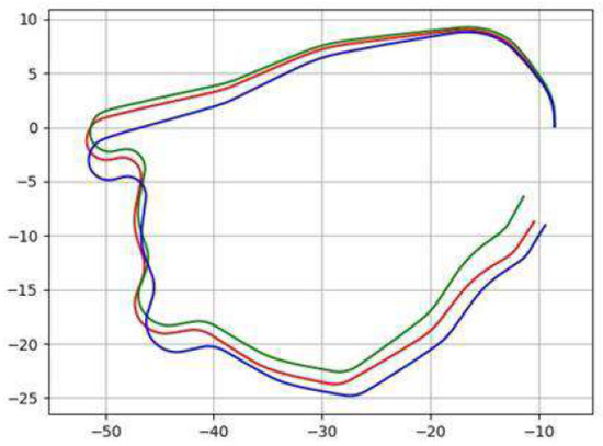
Figure 1.
Discrepancies in the state of the unmanned vehicle in the model with the state obtained using SLAM at the Gaussian noise level, with the same control without feedback.
In global planning, it is desirable that significant landmarks (obtaining unambiguous functions by the robot) appear in the area of the navigation trajectory, but are not an obstacle. At the same time, the global trajectory can be optimal in the sense of fault safety.
Optimal trajectory planning for autonomous robots has long been studied. Rosenblatt [15] developed a jet navigation system to enable multiple targets. Each goal is considered a behavior, and their task is to weigh a set of discrete motion controls based on its expected utility. The benefits from each behavior are also weighted by the central arbiter depending on the current mission of the system.
To be able to control the robot in real time, we need to update the map quickly enough [16]. This is very important for robots with fast dynamics, such as Figure 2 (the picture on the left) unmanned vehicle. To meet these requirements, you need to use accelerations, for example, using the CUDA GPU.
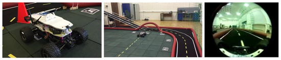
Figure 2.
Landmarks in the form of yellow markings, red cones, and radio frequency markers.
Our simple solution to refine and adjust the position and orientation of the mobile robot is to use a marker when initializing the unmanned vehicle and close loop. The disadvantage of the visual–inertial SLAM is its sensitivity to vibrations and in constantly changing light conditions. Between adjustments using radio frequency markers, the position and orientation of the mobile robot is correlated with the dynamic model of the mobile robot, and if the threshold is exceeded, the system uses the position and orientation of the model until it converges with the SLAM.
For dynamic obstacles in previous works [17], we used a trajectory generator and precalculated trajectories, which were selected by the cost function. The ASLAM-MPPI algorithm allows us to generate thousands of trajectories in real time and choose the one that takes into account the dynamic constraint (Figure 3). In Figure 3, we can see red, blue, and yellow fields; this is cost map. The light blue line is a trajectory of the ASLAM-MPPI method, visualized on RVIZ. The optimal trajectory has a violet color.
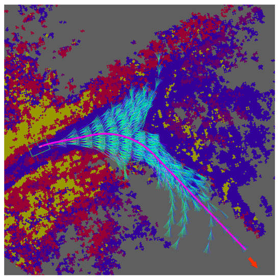
Figure 3.
The set of obtained trajectories, where the arrow indicates the direction of the optimal trajectory.
As a result, the ASLAM-MPPI algorithm works as follows:
- Using ASLAM algorithms, we obtain the local state of the unmanned vehicle (UV) and the employment map, taking into account dynamic obstacles;
- The A-star [18] algorithm calculates the global trajectory. Active SLAM includes terminal states in the circle of significant landmarks, for example, radio frequency markers;
- The ASLAM-MPI algorithm models predict, from the initial state, thousands of trajectories, taking into account the UV dynamics in the direction of the global trajectory. The prediction window depends on the calculated speed of dynamic obstacles;
- Using the cost function, the optimal trajectory is calculated according to a given criterion;
- The control corresponding to the optimal trajectory is applied;
- Then, the algorithm is repeated;
- If the UV localization exceeds the threshold of discrepancy with the forecast of the local state of the ASLAM-MPI algorithm, the localization system is corrected.
3. An example of using the method
Consider the movement of a robot with an Ackermann geometry chassis [19]:
where x, y are the coordinates of the center of the rear axis of the mobile robot; is its linear speed; is an angle of rotation around the axis x; is the rotation angle (positive counterclockwise); L is the distance between the front and rear axles of the wheels of the mobile robot.
The technology described above was tested in the robotics center of the Russian Academy of Sciences, where a polygon simulating an industrial facility with complex structures, ramps in the form of a steep hill, a bridge, and other restrictions is deployed. In Figure 4, we can see the part of the track with the form of bridge and a mobile robot with an Ackermann geometry chassis, which we use in our experiments.
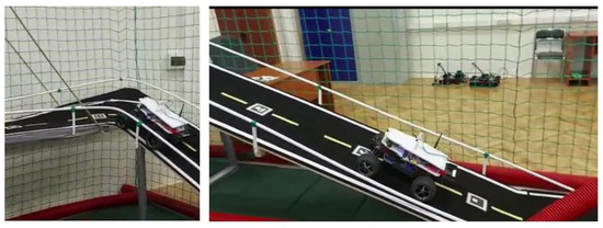
Figure 4.
The track.
Static phase restrictions are given:
where r is the obstacle dimensions; are the coordinates of the center of the obstacle.
If , where is the condition for recognizing labels in the algorithm, then the algorithm switches to another cost function, such as
where
- is from [17];
- , where stands for current coordinates and is distance to the recognized label;
- is a Heaviside function:
The dynamics model of the robot shown in Figure 2 (the picture on the left) was implemented on a neural network model structure having the following mathematical form:
where represents the configurable parameters of the neural network, including weight coefficients and offsets ; is the activation function of neurons in the output layer ; is the number of neurons in the hidden layer; is the activation function of neurons of the hidden layer; is the number of inputs.
Our neural network for the ASLAM-MPPI method includes two hidden layers with two nonlinearities, which means that the overall network configuration is 6-32-32-4. It takes as input four state variables (roll, longitudinal speed, transverse speed, course), as well as controlled steering and speed control, and they output the time derivative of the state variables. This network was trained on real data collected from the real polygon (Figure 4) in manual UV control mode. Stochastic gradient descent with ADAM was used for training.
As an embedded computing platform, NVIDIA Jetson TX2 was used with 256 CUDA cores and a four-core ARM Cortex-A57 processor, which made it possible to parallelize the computer network.
Experiments were conducted with ROS (melodic version) on a Linux computer with an Intel Core i7 processor, on which the MPPI algorithm was deployed. The control commands were transmitted via WiFi to the unmanned vehicle shown in Figure 2.
Closed trajectories were defined in the form of generated points in space, located on the dotted central track marking.
The absolute trajectory error (ATE) measurement showed the same error on the slide and on the horizontal plane, and was, on average, 0.99 percent of the length of the path traveled. The length of the path passing along the slide was 23.3 m. A deviation error of more than 0.03 m leads to accidents on the turns of the slide. Thus, the quality criterion of SLAM and control is the number of tracks passing through the slide.
In complex conditions, when spatial constraints severely constrict the space of acceptable movements, the strategy of selecting the state space for optimization is more efficient than sampling in the control space.
Thus, the quality criterion of the ASLAM-MPI algorithm is the number of tracks passing through the slide.
The experiment showed that the optimal passage of the slide firstly passes through the specified states, the exact definitions of which depend on the localization system of the robot.
We used the Intel Realsense T265, a standalone 6-degree-of-freedom tracking sensor that runs a visually-inertial SLAM algorithm that accurately evaluates movement with 6 degrees of freedom and obtains the positions and orientation of the tracking camera at 200 Hz, which is 10 times quicker than localization with the best-known ORB-SLAM2 algorithm [20].
Active SLAM shows an average of seven laps on a track with a slide without failures, which also depend on the control settings. A SLAM based on the Intel Realsense T265 tracking camera allows you to make only one lap, and on the second one, there is a failure due to an accumulated error, where the accumulation of errors leads to the inability to overcome turns on the slide. The slope of the slide is 45 degrees, and represents a serious limitation for the mobile robot. Figure 5 shows a track without a slide, because a SLAM method based on an Intel Realsense T265 security camera allows one to make 2–4 laps (depends on speed), after which a failure occurs due to an accumulated error.
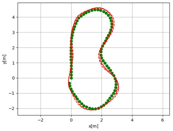
Figure 5.
An accumulated error on a track without a slide.
In Figure 6, we can see the polygon and its employment map.
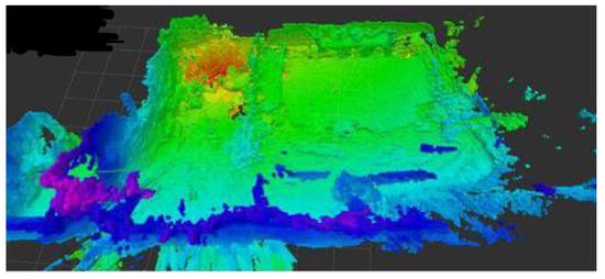
Figure 6.
Polygon employment map.
We see a further development of the method in accelerating the study of the robot’s map (like in Figure 6) with the help of autoencoders. We are also continuing to work on the automatic configuration of the cost function [17]. It has also been supposed to conduct experiments and compare the proposed method with previously known ones.
4. Conclusions
The result of the presented work is a new method for controlling an unmanned vehicle based on the choice of control in the state space that satisfies a given quality functional and is resistant to uncertain restrictions and interferences arising in a wide class for the SLAM method. The use of active SLAM allows, firstly, for a more reliable data association in the interface, including loop closures, which is important for correcting the orientation and posture of an unmanned vehicle, as well as detecting key points for odometry. Secondly, the method allows for controls to be developed based on navigation in unknown spaces. In addition, the method allows for the use of a variety of sensors for difficult conditions. At the same time, the method can use known cartographic information.
Classical control schemes are unable to predict costs and the corresponding trajectories (for example, PID controllers, LQR, iLQR). In addition, the formulation of the aggregate perception and action, as an optimization problem, has advantages in the reliability of the control system.
Our approach can be compared with the method [21] based on a predictive control model (MPC) with deep convolutional neural networks (CNN) for real-time scene understanding. A fully convolutional network is able to study the complex out-of-plane transformation required to project the observed image pixels onto the ground plane and predict the map of controlled objects in the area in front of the car. The solution is to train a deep neural network to convert visual inputs from a single monocular camera into a cost functions in a local coordinate system oriented to the robot is excellent. This cost map can then be directly introduced into the predictive model control algorithm. However, the disadvantage of the method may be nonvisited areas, where the training sample may not have enough reliable cost maps. The predictive controller (MPC) model uses only the information that it can see at the output of the neural network, and plans in advance for 1.5 s to issue a control signal. This 1.5-second time horizon leads to extremely timid behavior, because the available forward view has a short distance.
The practical result is the implementation of the method on a transport platform (see Figure 6) and the solution of the problem of following a global trajectory along a complex trajectory, including steep ascents and descents with spatial constraints that significantly narrow the choice of trajectory.
MPPI with deep convolutional neural networks cannot recognize ascents and descents from the slide without additional information. Thus, the cost map created by this method cannot be directly introduced into the predictive model control algorithm. Classical control schemes (for example, PID, LQR, and iLQR) can reliably track the global trajectory, but are not stable in cases of failures in the localization system.
As a result of conducted field experiments on a real UV, the ASLAM-MPPI method shows significant performance (algorithm speed, fault tolerance) compared to, for example, the ROS navigation stack [22].
Author Contributions
Conceptualization, A.N.D. and I.V.P.; methodology, A.N.D.; software, I.V.P.; formal analysis, A.N.D.; investigation, I.V.P.; resources, I.V.P.; data curation, A.N.D.; writing—original draft preparation, I.V.P.; writing—review and editing, A.N.D. and I.V.P. All authors have read and agreed to the published version of the manuscript.
Funding
This research received no external funding.
Institutional Review Board Statement
Not applicable.
Informed Consent Statement
Not applicable.
Data Availability Statement
Not applicable.
Conflicts of Interest
The authors declare no conflict of interest.
References
- Dellaert, F.; Kaess, V. Square Root SAM: Simultaneous Localization and Mapping via Square Root Information Smoothing. Int. J. Robot. Res. 2006, 25, 1181–1203. [Google Scholar] [CrossRef]
- Kaess, M.; Johannsson, H.; Roberts, R.; Ila, V.; Leonard, J.J.; Dellaert, F. iSAM2: Incremental Smoothing and Mapping Using the Bayes Tree. Int. J. Robot. Res. 2012, 31, 217–236. [Google Scholar] [CrossRef]
- Thrun, S.; Montemerlo, M. The GraphSLAM Algorithm With Applications to Large-Scale Mapping of Urban Structures. Int. J. Robot. Res. 2005, 25, 403–430. [Google Scholar] [CrossRef]
- Montemerlo, M.; Thrun, S.; Koller, D.; Wegbreit, B. FastSLAM: A factored solution to the simultaneous localization and mapping problem. In Proceedings of the AAAI National Conference on Artificial Intelligence, Edmonton, AL, Canada, 28 July–1 August 2002; pp. 593–598. [Google Scholar]
- Kschischang, F.R.; Frey, B.J.; Loeliger, H.A. Factor Graphs and the Sum-Product Algorithm. IEEE Trans. Inf. Theory 2001, 47, 498–519. [Google Scholar] [CrossRef]
- Cadena, C.; Carlone, L.; Carrillo, H.; Latif, Y.; Scaramuzza, D.; Neira, J.; Reid, I.; Leonard, J.J. Past, Present, and Future of Simultaneous Localization And Mapping: Towards the Robust-Perception Age. IEEE Trans. Robot. 2016, 32, 1309–1332. [Google Scholar] [CrossRef]
- Williams, G.; Goldfain, B.; Drews, P.; Rehg, J.M.; Theodorou, E.A. Autonomous Racing with AutoRally Vehicles and Differential Games. arXiv 2017, arXiv:1707.04540. [Google Scholar]
- Bajcsy, R. Active Perception. Proc. IEEE 1988, 76, 966–1005. [Google Scholar] [CrossRef]
- Leung, C.; Huang, S.; Dissanayake, G. Active SLAM using Model Predictive Control and Attractor Based Exploration. In Proceedings of the IEEE/RSJ International Conference on Intelligent Robots and Systems, Beijing, China, 9–15 October 2006; pp. 5026–5031. [Google Scholar]
- Ardón, P.; Kushibar, K.; Peng, S. A Hybrid SLAM and Object Recognition System for Pepper Robot. arXiv 2019, arXiv:1903.00675. Available online: https://github.com/PaolaArdon/Salt-Pepper (accessed on 10 September 2022).
- Leung, C.; Huang, S.; Kwok, N.; Dissanayake, G. Planning Under Uncertainty using Model Predictive Control for Information Gathering. Robot. Auton. Syst. 2006, 54, 898–910. [Google Scholar] [CrossRef]
- Williams, G.; Drews, P.; Goldfain, B.; Rehg, J.M.; Theodorou, E.A. Aggres-sive driving with model predictive path integral control. In Proceedings of the IEEE International Conference on Robotics and Automation, Jeju Island, Republic of Korea, 27–31 August 2016; pp. 1433–1440. [Google Scholar]
- Williams, G.; Aldrich, A.; Theodorou, E.A. Model predictive path integral control: From theory to parallel computation. J. Guid. Control. Dyn. 2017, 40, 1–14. [Google Scholar] [CrossRef]
- AutoRally. Available online: https://github.com/AutoRally/autorally (accessed on 12 July 2022).
- Rosenblatt, J.K. Optimal selection of uncertain actions by maximizing expected utility. In Proceedings of the IEEE International Symposium on Computational Intelligence in Robotics and Automation, Monterey, CA, USA, 8–9 November 1999; pp. 95–100. [Google Scholar]
- Guizilini, V.; Ramos, F. Towards real-time 3d continuous occupancy mapping using hilbert maps. Int. J. Robot. Res. 2018, 37, 566–584. [Google Scholar] [CrossRef]
- Daryina, A.N.; Prokopiev, I.V. Unmanned vehicle’s control real-time method based on neural network and selection function. Procedia Comput. Sci. 2021, 186, 217–226. [Google Scholar] [CrossRef]
- Hart, P.E.; Nilsson, N.J.; Raphael, B. Correction to A Formal Basis for the Heuristic Determination of Minimum Cost Paths. Sigart Newsl. 1972, 37, 28–29. [Google Scholar] [CrossRef]
- Kuwata, Y.; Teo, J.; Karaman, S.; Fiore, G.; Frazzoli, E.; How, J.P. Motion planning in complex environments using closed-loop prediction. Presented at the AIAA Guidance, Navigation and Control Conference and Exhibit, Honolulu, HI, USA, 18–21 August 2008. [Google Scholar]
- Mur-Artal, R.; Tardós, J.D. ORB-SLAM2: An open-source SLAM system for monocular, stereo, and RGB-D cameras. IEEE Trans. Robot. 2017, 33, 1255–1262. [Google Scholar] [CrossRef]
- Drews, P.; Williams, G.; Goldfain, B.; Theodorou, E.A.; Rehg, J.M. Aggressive Deep Driving: Combining Convolutional Neural Networks and Model Predictive Control. arXiv 2017, arXiv:1707.05303. [Google Scholar]
- ROS. Available online: https://wiki.ros.org/navigation (accessed on 24 August 2022).


Disclaimer/Publisher’s Note: The statements, opinions and data contained in all publications are solely those of the individual author(s) and contributor(s) and not of MDPI and/or the editor(s). MDPI and/or the editor(s) disclaim responsibility for any injury to people or property resulting from any ideas, methods, instructions or products referred to in the content. |
© 2023 by the authors. Licensee MDPI, Basel, Switzerland. This article is an open access article distributed under the terms and conditions of the Creative Commons Attribution (CC BY) license (https://creativecommons.org/licenses/by/4.0/).