Optimal Design of a Reliability Experiment Based on the Wiener Degradation Model under Limitations of the Degradation Index ^†

Abstract

There are many degradation models that are used in reliability analyses. The Wiener degradation model is the most popular across different applications. In this paper, we propose an approach for searching for an optimal design on the basis of the Wiener degradation model. The distinguishing feature of the approach is that the condition that the degradation index cannot exceed a critical level has been taken into account. The elements of the conditional Fisher information matrix have been obtained. This enables us to calculate the optimal stress levels by maximizing the functional of the conditional Fisher information matrix. Moreover, a degradation analysis of light-emitting diodes (LEDs) has been considered.

1. Introduction

A high reliability and long useful lifetime are the most important features of modern equipment. Such requirements make reliability analyses of devices more complicated. Classical methods based on failure data are not suitable for equipment reliability analyses because not all devices fail during experiments. In this case, other characteristics of the equipment can be used, for example, the degradation index or the so-called health index, which demonstrate the condition of the product under study. The Wiener degradation model is the most popular model that can be applied in the case of a non-monotonic degradation path [1,2,3,4,5,6,7,8]. The gamma and inverse Gaussian degradation models are often mentioned in scientific articles [9,10], but can be used for solving tasks where the degradation index only has positive increments.

Despite the fact that observed degradation data allow us to carry out reliability analyses without failure time data, the duration of the experiment can be quite long. Thus, the observation of degradation data during accelerated life testing is widely used in many papers. To conduct an accelerated life test, it is necessary to increase the stress level on a part of the devices, such as voltage, pressure, temperature, etc. [11].

Since in practice it may often be necessary to repeat such an analysis, many scientists have thought about how to optimize the cost and duration of experiment, that is, how to obtain the optimal design for further analysis. The first step for optimal planning was made by R. A. Fisher [12]. Since the 1950s, a lot of scientists have persistently solved the problem of optimal experimental design to obtain both the optimal stress levels and the number of studied units under restrictions on the allowable stress levels, the cost and duration of the experiment [13]. In [14,15,16], we emphasized that the choice of time points for measuring the degradation index significantly affects the accuracy of the maximum likelihood estimates for the Wiener degradation model parameters. The optimal distribution of measurement time points depends on the model describing the degradation process as well as the experimental conditions, such as the experiment duration, stress levels and the minimum time interval between measurements of the degradation index [14,15,16]. In [16], we suggested an algorithm for constructing A- and D-optimal designs based on the Wiener degradation model, which includes determining the optimal stress levels, the number of tested devices and the time moments for measuring the degradation index. However, in that paper, we did not consider the fact that in real life the observation of the object is terminated when the degradation path reaches the critical value.

Thus, in this paper, we develop an algorithm for constructing optimal designs based on the Wiener degradation model, which includes determining the optimal stress levels considering the limitation of the degradation index.

2. The Wiener Degradation Model in Reliability Analysis

Let us assume that the observed stochastic process $Z\left(t\right)$ is a stochastic process with independent increments and $Z\left(0\right)=0$. For the Wiener degradation model, increments have a normal distribution with the probability density function:

$$f(u,{\theta }_1,{\theta }_2)=\frac{1}{{\theta }_2\sqrt{2\pi }}exp\left(-\frac{{(u-{\theta }_1)}^2}{2{\theta }_2^2}\right),$$

(1)

where ${\theta }_1=\mu (\rho (t+\Delta \left(t\right))-\rho \left(t\right))$ is the shift parameter, ${\theta }_2=\sigma \sqrt{\left(\rho \right(t+\Delta \left(t\right))-\rho (t\left)\right)}$ is the scale parameter, $\sigma >0$ and $\rho \left(t\right)$ is a positive increasing function.

Let us denote the vector of stresses (which are also often referred to as covariates) as $x={(x^1,x^2,\cdots ,x^m)}^T$. The range of values for each covariate $x^j,j=\overline{1,m}$ is determined by the conditions of the experiment. In this paper, the degradation process $Z\left(t\right)$ is supposed to be observed under a constant time stress. Here, we assume that the covariate x influences the degradation paths as in the accelerated failure time model:

$$Z_x\left(t\right)=Z\left(\frac{t}{r(x,\beta )}\right),$$

where $r(x,\beta )$ is a the positive covariate function and $\beta ={({\beta }_1,{\beta }_2,\cdots ,{\beta }^m)}^T$ is the vector of regression parameters. The mathematical expectation of the degradation process $Z_x\left(t\right)$ is denoted by

$$E\left(Z_x\left(t\right)\right)=\mu \rho \left(\frac{t}{r(x,\beta )},\gamma \right).$$

The time to failure, which depends on covariate x, is defined as:

$$\tau =sup\left(t:Z_x\left(t\right)<z_0\right),$$

where $z_0$ is the critical value of the degradation index. Then, the reliability function can be represented as:

$$S\left(t\right)=P\{\tau <t\}=P(Z_x\left(t\right)<z_0)=\mathsf{\Phi }\left(\frac{z_0-\mu \rho (t/r(x;\beta );\gamma )}{\sigma \rho (t/r(x;\beta )}\right).$$

Suppose the experiment is running over time T. The degradation index values are measured at time points $0=t_0,t_1,\dots ,t_k=T$.

Let us denote the sample of independent degradation index increments with covariates as the following:

$${\mathbf{X}}_{\mathbf{n}}=\{(\Delta Z_{1j},x_1),\dots ,(\Delta Z_{nj},x_n),j=\overline{1,k}\},$$

where k is the number of measurements of the degradation index for each object, $x_i$ is the value of the covariate vector for the i-th object and $\Delta Z_{ij}=Z_i\left(t_j\right)-Z_i\left(t_{j-1}\right)$ is the increment of the degradation index during the time from $t_{j-1}$ to $t_j$.

the unknown parameters of the model can be estimated using the maximum likelihood method:

$$lnL\left({\mathbf{X}}_{\mathbf{n}}\right)=-nk(ln\sqrt{2\pi }+ln\sigma )-\frac{n}{2}\sum _{j=1}^{k}ln\left(\rho \left(t_{j+1}\right)-\rho \left(t_j\right))\right)-$$

$$\frac{1}{2{\sigma }^2}\sum _{i=1}^n\sum _{j=1}^k\frac{{\left[\Delta Z_{ij}-\mu \left(\rho \left(t_{j+1}\right)-\rho \left(t_j\right))\right)\right]}^2}{\left(\rho \left(t_{j+1}\right)-\rho \left(t_j\right))\right)}.$$

3. Optimal Design of Experiments

We denote the experiment design as a set of values $\xi =\{x_{\left(1\right)},x_{\left(2\right)},\cdots x_{\left(q\right)}\},$ where $x_{\left(i\right)}$ are the reference points of the design. All objects of the sample are divided into q groups corresponding to different values of the covariate vector (reference points of the design). Thus, the problem of direct searching for an optimal design can be written as follows:

$$\left\{\begin{array}{c}M\left(I\right(\xi \left)\right)\to max,\hfill \\ x_{min}⩽x_{\left(i\right)}⩽x_{max},\hfill \end{array}\right.$$

where $M(.)$ is some functional of the Fisher information matrix and $x_{min}$, $x_{max}$ are the minimum and maximum values of stress levels determined by the conditions of experiment. The construction of the D-optimal design is based on maximizing the determinant of the Fisher information matrix:

$$M\left(I\right(\xi \left)\right)=det\left(I\right(\xi \left)\right).$$

In [16], we did not take into account the fact that in real life the observation of the object is terminated when the degradation path reaches a critical value. To solve this problem, the conditional density function should be considered: $f_{\Delta Z_{ij}}\left(u\right|Z_k⩽z_0)$, where $Z_k=Z_x\left(t_k\right)$.

However, the calculation of the conditional density function requires the calculation of k-fold integrals, which is a composite computational problem. Thus, we propose to use only the last observation $Z_k$ of each degradation path for constructing an optimal design, which enables us to determine the optimal stress levels.

We have obtained the mathematical expectation of the second derivatives with respect to the parameters of the likelihood function to obtain elements of the Fisher information matrix under condition $Z_{t_k}⩽z_0$:

$$I\left(\xi \right)=-E\left(\frac{{\partial }^{2}lnf\left(z_k\right|z_k⩽z_0)}{\partial \theta \partial {\theta }^T}\right),$$

where

$$ln{f}_{Z_k}\left(u\right|Z_k⩽z_0)=ln{f}_{Z_k}\left(z_k\right)-ln{F}_{Z_k}\left(z_0\right).$$

We calculated elements of the Fisher information matrix:

$$I_{11}=\frac{2n}{{\sigma }^2}-\left[3\frac{{(z_0-\mu \rho \left(t_k\right))}^2}{2{\sigma }^4\rho \left(t_k\right)}-\frac{{(z_0-\mu \rho \left(t_k\right))}^4}{4{\sigma }^6{\rho }^2\left(t_k\right)}{c}_2\right]c_1-\frac{c_1}{F_{Z_k}}\frac{{(z_0-\mu \rho \left(t_k\right))}^4}{4{\sigma }^6{\rho }^2\left(t_k\right)};$$

$$I_{12}=-\left[2\frac{(z_0-\mu \rho \left(t_k\right))}{{\sigma }^2}-\frac{{(z_0-\mu \rho \left(t_k\right))}^3}{2{\sigma }^5\rho \left(t_k\right)}{c}_2\right]c_1-\frac{c_1}{F_{Z_k}}\frac{{(z_0-\mu \rho \left(t_k\right))}^3}{2{\sigma }^5\rho \left(t_k\right)};$$

$$I_{13}=\frac{1}{\sigma }\sum _{i=1}^q\frac{1}{\rho \left(t_{ik}\right)}\frac{\partial \rho \left(t_{ik}\right)}{\partial \gamma }-\left[\frac{(z_0^2-{\mu }^2{\rho }^2\left(t_k\right))}{{\sigma }^3{\rho }^2\left(t_k\right)}\frac{\partial \rho \left(t_k\right)}{\partial \gamma }\frac{{(z_0-\mu \rho \left(t_k\right))}^2(z_0^2-{\mu }^2{\rho }^2\left(t_k\right))}{4{\sigma }^5{\rho }^3\left(t_k\right)}\frac{\partial \rho }{\partial \gamma }{c}_2\right]c_1-$$

$$\frac{c_1}{F_{Z_k}}\frac{{(z_0-\mu \rho \left(t_k\right))}^2(z_0^2-{\mu }^2{\rho }^2\left(t_k\right))}{4{\sigma }^5{\rho }^3\left(t_k\right)}\frac{\partial \rho }{\partial \gamma };$$

$$I_{14}=\frac{1}{\sigma }\sum _{i=1}^q\frac{1}{\rho \left(t_{ik}\right)}\frac{\partial \rho \left(t_{ik}\right)}{\partial \beta }-\left[\frac{(z_0^2-{\mu }^2{\rho }^2\left(t_k\right))}{{\sigma }^3{\rho }^2\left(t_k\right)}\frac{\partial \rho \left(t_k\right)}{\partial \beta }-\frac{{(z_0-\mu \rho \left(t_k\right))}^2(z_0^2-{\mu }^2{\rho }^2\left(t_k\right))}{4{\sigma }^5{\rho }^3\left(t_k\right)}\frac{\partial \rho }{\partial \beta }{c}_2\right]c_1-$$

$$\frac{c_1}{F_{Z_k}}\frac{{(z_0-\mu \rho \left(t_k\right))}^2(z_0^2-{\mu }^2{\rho }^2\left(t_k\right))}{4{\sigma }^5{\rho }^3\left(t_k\right)}\frac{\partial \rho }{\partial \beta };$$

$$I_{22}=\frac{1}{{\sigma }^2}\sum _{i=1}^q\rho \left(t_{ik}\right)-\left[\frac{\rho \left(t_k\right)}{{\sigma }^2}-\frac{{(z_0-\mu \rho \left(t_k\right))}^2}{{\sigma }^4}{c}_2\right]c_1-\frac{c_1}{F_{Z_k}}\frac{{(z_0-\mu \rho \left(t_k\right))}^2}{{\sigma }^4};$$

$$I_{23}=\frac{{\mu }^2}{{\sigma }^2}\sum _{i=1}^q\frac{\partial \rho t_{ik}}{\partial \gamma }-\left[\frac{\mu }{{\sigma }^2}\frac{\partial \rho \left(t_k\right)}{\partial \gamma }-\frac{(z_0-\mu \rho \left(t_k\right))(z_0^2-{\mu }^2{\rho }^2\left(t_k\right))}{2{\sigma }^4{\rho }^2\left(t_k\right)}\frac{\partial \rho }{\partial \gamma }{c}_2\right]c_1-$$

$$\frac{c_1}{F_{Z_k}}\frac{(z_0-\mu \rho \left(t_k\right))(z_0^2-{\mu }^2{\rho }^2\left(t_k\right))}{2{\sigma }^4{\rho }^2\left(t_k\right)}\frac{\partial \rho }{\partial \gamma };$$

$$I_{24}=\frac{{\mu }^2}{{\sigma }^2}\sum _{i=1}^q\frac{\partial \rho t_{ik}}{\partial \beta }-\left[\frac{\mu }{{\sigma }^2}\frac{\partial \rho \left(t_k\right)}{\partial \beta }-\frac{(z_0-\mu \rho \left(t_k\right))(z_0^2-{\mu }^2{\rho }^2\left(t_k\right))}{2{\sigma }^4{\rho }^2\left(t_k\right)}\frac{\partial \rho }{\partial \beta }{c}_2\right]c_1-$$

$$\frac{c_1}{F_{Z_k}}\frac{(z_0-\mu \rho \left(t_k\right))(z_0^2-{\mu }^2{\rho }^2\left(t_k\right))}{2{\sigma }^4{\rho }^2\left(t_k\right)}\frac{\partial \rho }{\partial \beta };$$

$$\begin{array}{c}{I}_{33}=\sum _{i=1}^q{\left(\frac{\partial \rho \left(t_{ik}\right)}{\partial \gamma }\right)}^2\left(\frac{1}{2{\rho }^2\left(t_{ik}\right)}+\frac{{\mu }^2}{{\sigma }^2\rho \left(t_{ik}\right)}\right)-\left[\frac{1}{{\sigma }^2{\rho }^3\left(t_k\right)}\right(z_0^2{\left(\frac{\partial \rho \left(t_k\right)}{\partial \gamma }\right)}^2-\hfill \\ \hfill \frac{{\partial }^2\rho \left(t_k\right)}{\partial {\gamma }^2}\frac{\left(z_0^2\rho -{\mu }^2{\rho }^3\right)}{2})-\frac{{(z_0^2-{\mu }^2{\rho }^2\left(t_k\right))}^2}{4{\sigma }^4{\rho }^4\left(t_k\right)}\frac{\partial \rho }{\partial \gamma }{c}_2]c_1-\frac{c_1}{F_{Z_k}}\frac{{(z_0^2-{\mu }^2{\rho }^2\left(t_k\right))}^2}{4{\sigma }^4{\rho }^4\left(t_k\right)}\frac{\partial \rho }{\partial \gamma };\end{array}$$

$$I_{34}=\sum _{i=1}^q\left(\frac{\partial \rho \left(t_{ik}\right)}{\partial \gamma }\frac{\partial \rho \left(t_{ik}\right)}{\partial \beta }\right)\left(\frac{1}{2{\rho }^2\left(t_{ik}\right)}+\frac{{\mu }^2}{{\sigma }^2\rho \left(t_{ik}\right)}\right)-\left[\frac{1}{{\sigma }^2{\rho }^3\left(t_k\right)}\right(z_0^2\frac{\partial \rho \left(t_k\right)}{\partial \beta }\frac{\partial \rho \left(t_k\right)}{\partial \gamma }-$$

$$\frac{{\partial }^2\rho }{\partial \gamma \partial \beta }\frac{\left(z_0^2\rho -{\mu }^2{\rho }^3\left(t_k\right)\right)}{2})--\frac{{(z_0^2-{\mu }^2{\rho }^2\left(t_k\right))}^2}{4{\sigma }^4{\rho }^4\left(t_k\right)}\frac{\partial \rho }{\partial \gamma }\frac{\partial \rho }{\partial \beta }{c}_2]c_1-$$

$$-\frac{c_1}{F_{Z_k}}\frac{{(z_0^2-{\mu }^2{\rho }^2\left(t_k\right))}^2}{4{\sigma }^4{\rho }^4\left(t_k\right)}\frac{\partial \rho }{\partial \gamma }\frac{\partial \rho }{\partial \beta };$$

$$I_{44}=\sum _{i=1}^q{\left(\frac{\partial \rho \left(t_{ik}\right)}{\partial \beta }\right)}^2\left(\frac{1}{2{\rho }^2\left(t_{ik}\right)}+\frac{{\mu }^2}{{\sigma }^2\rho \left(t_{ik}\right)}\right)-\left[\frac{1}{{\sigma }^2{\rho }^3\left(t_k\right)}\right(z_0^2{\left(\frac{\partial \rho \left(t_k\right)}{\partial \beta }\right)}^2-$$

$$\frac{{\partial }^2\rho \left(t_k\right)}{\partial {\beta }^2}\frac{\left(z_0^2\rho -{\mu }^2{\rho }^3\right)}{2})-\frac{{(z_0^2-{\mu }^2{\rho }^2\left(t_k\right))}^2}{4{\sigma }^4{\rho }^4\left(t_k\right)}\frac{\partial \rho }{\partial \beta }{c}_2]c_1-$$

$$-\frac{c_1}{F_{Z_k}}\frac{{(z_0^2-{\mu }^2{\rho }^2\left(t_k\right))}^2}{4{\sigma }^4{\rho }^4\left(t_k\right)}\frac{\partial \rho }{\partial \beta };$$

where

$$c_1=\frac{1}{2\sqrt{\pi }}\frac{\sigma \sqrt{2\rho \left(t_{ik}\right)}}{(z_0-\mu \rho \left(t_{ik}\right))}exp\left(-\frac{{(z_0-\mu \rho \left(t_{ik}\right))}^2}{2{\sigma }^2\rho \left(t_{ik}\right)}\right),c_2=\frac{{\sigma }^2\rho \left(t_{ik}\right)}{{(z_0-\mu \rho \left(t_{ik}\right))}^2}+1.$$

The function of normal distribution equals:

$$F_{Z_k}={\int }_{-\infty }^{z_0}\frac{1}{\sigma \sqrt{2\pi \rho }}exp\left(-\frac{{(z-\mu \rho \left(t_{ik}\right))}^2}{2{\sigma }^2\rho \left(t_{ik}\right)}\right)dz=0.5+0.5\mathsf{\Gamma }\left(0.5,\frac{{(z_0-\mu \rho \left(t_{ik}\right))}^2}{2{\sigma }^2\rho \left(t_{ik}\right)}\right).$$

4. Optimal Design for a Light-Emitting Diode Reliability Test

In [16], we considered the problem of a reliability analysis for LEDs. Following the proposed algorithm, the D-optimal design for testing the reliability of LEDs has been obtained. It was shown that the determinant of the Fisher information matrix significantly increased for the optimal design in comparison with the initial design. However, the previous algorithm did not take into account the fact that in real life the observation of the object is terminated when the degradation path reaches the critical value. In this paper, we have improved the algorithm on the basis of the conditional Fisher information matrix and have analyzed how the optimal design has been changed.

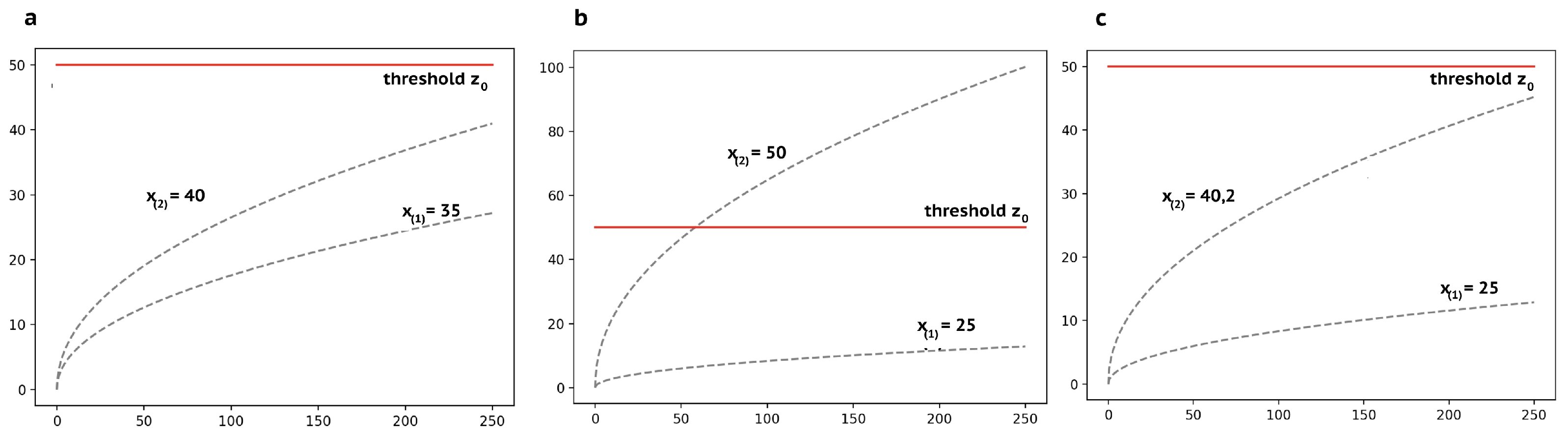
Let us describe the initial conditions of the experiment. LED lighting offers many benefits for industrial and commercial businesses that are interested in reducing their energy usage and costs. The experiment involves the observation of 24 LEDs for 250 h. The normal stress level of an LED is 25mA. However, the LEDs were tested at two levels of electric current (40 mA and 35 mA) to conduct an accelerated reliability experiment. When the light intensity decreases by 50 percent, the failure of the unit is recorded.

As it was shown in [16], the date can be described by the Wiener degradation model with a log-linear trend function and a power covariate function:

$$f_{\Delta Z_{ij}}\left(u\right)=\frac{1}{\sigma \sqrt{2\pi \Delta \rho \left(t_{ij}\right)}}exp\left(-\frac{{(u-\mu \Delta \rho \left(t_{ij}\right))}^2}{2{\sigma }^2\Delta \rho \left(t_{ij}\right)}\right),$$

where $\Delta \rho \left(t_{ij}\right)={\left(\frac{t_{ij}}{e^{x\beta }}\right)}^{\gamma }-{\left(\frac{t_{i(j-1)}}{e^{x\beta }}\right)}^{\gamma }$ with parameters $\sigma =0.49,\mu =0.11;\gamma =0.48$; and $\beta =-0.17.$ Let us find the optimal experiment design basing on the Fisher information matrix presented in Section 3:

$$\left\{\begin{array}{c}M\left(I\right(\xi \left)\right)\to max,\hfill \\ 25⩽x_{\left(i\right)}⩽50.\hfill \end{array}\right.$$

(2)

In Figure 1, the trend functions corresponding to the initial design, the optimal design obtained in [16] and the optimal design obtained on the basis of the conditional Fisher information matrix are presented.

As can be seen from Figure 1b, the optimal design obtained in [16] includes stress levels equal to the minimum and maximum levels determined by the conditions of the experiment (2). However, in practice, a large amount of information on the degradation path will be lost since the object observation should be terminated when the degradation path reaches the threshold.

Figure 1c clearly illustrates that in the case of using the conditional Fisher information matrix, the reference points of the optimal design correspond to the minimum stress level and the maximum possible stress level under limitations of the degradation index.

Let us check how the determinant of the estimated conditional Fisher information matrix has changed with the new reference points of the design: $M\left(I\left({\xi }_0\right)\right)=det\left(I\left({\xi }_0\right)\right)=2e+12,M\left(I\left({\xi }^{*}\right)\right)=det\left(I\left({\xi }^{*}\right)\right)=9e+13.$ On the basis of the obtained result, it is possible to conclude that the accuracy of parameter estimates has increased, as the functional of the conditional Fisher information matrix has significantly increased.

5. Conclusions

In this paper, we have obtained the elements of a conditional Fisher information matrix for the Wiener degradation model under the condition that the degradation path is limited: $Z_x\left(t\right)⩽z_0$. It is proposed that the optimal stress levels could be obtained by maximizing the functional of the conditional Fisher information matrix. Reliability analyses for LEDs have been considered as an example. Following the proposed approach, the D-optimal design for testing the reliability of LEDs has been obtained. On the basis of the obtained result, it is possible to conclude that the accuracy of parameter estimates has increased, as the functional of the conditional Fisher information matrix has significantly increased.

References

- Si, X.-S.; Wang, W.; Hu, C.-H.; Chen, M.-Y.; Zhou, D.-H. A Wiener-process-based degradation model with a recursive filter algorithm for remaining useful life estimation. Mech. Syst. Signal Process. 2013, 35, 219–237. [Google Scholar] [CrossRef]
- Zhou, S.; Tang, Y.; Xu, A. A generalized Wiener process with dependent degradation rate and volatility and time-varying mean-to-variance ratio. Reliab. Eng. Syst. Saf. 2021, 216. [Google Scholar] [CrossRef]
- Wang, Z.; Li, J.; Ma, X.; Zhang, Y.; Fu, H.; Krishnaswamy, S. A Generalized Wiener Process Degradation Model with Two Transformed Time Scales. Qual. Reliab. Eng. Int. 2016, 33. [Google Scholar] [CrossRef]
- Peng, C.Y.; Tseng, S.T. Mis-Specification Analysis of Linear Degradation Models. IEEE Trans. Reliab. 2009, 3, 444–455. [Google Scholar] [CrossRef]
- Tang, J.; Su, T. Estimating failure time distribution and its parameters based on intermediate data from a Wiener degradation model. Nav. Res. Logist. 2008, 3, 265–276. [Google Scholar] [CrossRef]
- Ye, Z.-S.; Chen, N.; Shen, Y. A new class of Wiener process models for degradation analysis. Reliab. Eng. Syst. Saf. 2015, 139, 58–67. [Google Scholar] [CrossRef]
- Hu, C.-H.; Lee, M.-Y.; Tang, J. Optimum step-stress accelerated degradation test for Wiener degradation process under constraints. Eur. J. Oper. Res. 2015, 241, 412–421. [Google Scholar] [CrossRef]
- Chaluvadi, V. Accelerated Life Testing of Electronic Revenue Meters. Master’s Thesis, Clemson University, Clemson, SC, USA, 2008. [Google Scholar]
- Chetvertakova, E.S.; Chimitova, E.V. Testing significance of random effects for the gamma degradation model. Anal. Data Process. Syst. 2021, 3, 129–142. [Google Scholar] [CrossRef]
- Chimitova, E.V.; Chetvertakova, E.S.; Sergeeva, S.A.; Osinceva, E.A. A comparative analysis of the wiener, gamma and inverse Gaussian degradation models. In Proceedings of the International Workshop Applied Methods of Statistical Analysis, Nonparametric Methods in Cybernetics and System Analysis (AMSA’2017), Krasnoyarsk, Russia, 18–22 September 2017; pp. 160–167. [Google Scholar]
- Liao, C.M.; Tseng, S.T. Optimal design for step-stress accelerated degradation tests. IEEE Trans Reliab. 2006, 1, 59–66. [Google Scholar] [CrossRef]
- Fisher, R.A. The Design of Experiments, 6th ed.; Oliver and Boyd: London, UK, 1951; 256p. [Google Scholar]
- Wu, S.J.; Chang, C.T. Optimal design of degradation tests in presence of cost constraint. Reliab. Eng. Syst. Saf. 2002, 76, 109–115. [Google Scholar] [CrossRef]
- Osintseva, E.A.; Chimitova, E.V. Informacionnaya matrica Fishera dlya vinerovskoj degradacionnoj modeli s uchetom ob’yasnyayushchih peremennyh. [Fisher’s information matrix for the Wiener degradation model with covariate]. In Proceedings of the Russian Scientific and Technical Conference on the Information Processing and Mathematical Modeling, Novosibirsk, Russia, 25–26 April 2019; pp. 92–97. (In Russian). [Google Scholar]
- Osintseva, E.A.; Chimitova, E.V. Postroenie optimal’nyh planov eksperimenta na osnove vinerovskoj degradacionnoj modeli. [Construction of optimal experimental designs based on the Wiener degradation model]. In Proceedings of the Russian Scientific and Technical Conference on the Information Processing and Mathematical Modeling, Novosibirsk, Russia, 25–26 April 2018; pp. 75–85. (In Russian). [Google Scholar]
- Osintseva, E.; Chimitova, E. Optimal Design of Reliability Experiment Based on the Wiener Degradation Model with Covariates. Vestnik Tomskogo Gosudarstvennogo Universiteta. Upravlenie Vychislitelnaja Tehnika i Informatika. 2022, pp. 23–33. Available online: https://elibrary.ru/item.asp?id=49330076 (accessed on 4 July 2022).