Assessment of Inverse Distance Weighting and Local Polynomial Interpolation for Annual Rainfall: A Case Study in Peninsular Malaysia ^†

Abstract

Rainfall data are crucial in hydrology models. In this study, the assessment of two spatial interpolation approaches of Inverse Distance Weighting (IDW) and Local Polynomial Interpolation (LPI) for rainfall in Peninsular Malaysia was conducted. The daily precipitation for 515 rainfall stations across Peninsular Malaysia during 2011–2020 was used as the reference data. The performance of IDW and LPI was evaluated by the computation of the coefficient of determination (R²), the mean absolute error (MAE), and the root mean square error (RMSE). The results show that LPI methods surpass IDW methods on the annual scale rainfall interpolations in Peninsular Malaysia by exhibiting a better statistical evaluation.

1. Introduction

Rainfall data are crucial for hydrological modeling when anticipating extreme precipitation events such as droughts and floods and assessing the quantity and quality of the surface and groundwater. However, in most situations, the precipitation measurement station network is poor, and the data supplied are insufficient to define the highly variable precipitation and its geographical distribution. This is particularly true in underdeveloped nations such as Algeria, where the complexity of rainfall distribution is compounded by measuring challenges. As a result, the methods for estimating rainfall in regions where rainfall has not been recorded must be established based on data from nearby meteorological stations [1,2,3].

One of the ways to forecast rainfall is by using spatial interpolation techniques. In environmental management, geographic continuous data (or spatial continuous surfaces) are important for planning, risk assessment, and decision-making. They are, however, not always widely available and can be difficult and expensive to obtain, especially in hilly or deep-water places. During field surveys, environmental data are frequently collected from point sources. Environmental managers, on the other hand, typically require precise geographic continuous data throughout an area to make effective and confident choices, whereas scientists require accurate spatial and continuous data across a region to make justified conclusions [4,5,6].

The spatial continuous data of environmental variables have become more significant as geographic information systems (GIS) and modeling approaches have become more powerful for the conservation of natural resources and biological conservation. As a result, attribute values at unsampled places must be inferred, requiring spatial interpolation from data sets for spatial continuous data. Once the variational surface has various degrees of resolution, the cell density, or inclination other than what is required, is also necessary [7]. Furthermore, when a continuous region is presented by a different information type than what is required, and the confirming data do not completely cover the region of interest, spatial interpolation is required [8]. Therefore, this study aimed to investigate accurate and efficient spatial interpolation methods to evaluate rainfall data.

2. Methodology

The historical daily precipitation data (2011–2020) of 550 rain gauges were obtained from the Department of Irrigation and Drainage Malaysia (DID). Since rain gauges only show the point sampling of a storm’s areal spread, before using the data, it is necessary to undergo the process of a quality check, which is important to ensure that rainfall data are consistent. Stations with no missing data were acceptable in this study, while stations with missing data were further categorized into categories of less than 10% and more than 10%. According to Burhanuddin et al. [9], only data with a low quantity of missing data (less than 10%) could be considered good quality data, and thus, stations with more than 10% of missing data were directly eliminated from the study. Apart from this, according to Chow et al. [10], for station X with less than 10% missing data, the arithmetic procedure could be adopted to estimate the missing observation of station X.

$$\stackrel{-}{p}=\frac{{\sum }_{i=1}^{n}p}{n}$$

(1)

$\stackrel{-}{p}=$ combined mean for the rainfall station

$n=$ number of the rainfall station

$i=$ individual rainfall station

Hence, in this study, missing data were filled with precipitation values from the nearest stations, which tended to have similar characteristics using the arithmetic procedure. Next, the daily precipitation was aggregated into yearly, monthly, and daily scales for better comparison. After the process of data acquisition, a total of 515 stations were applied to the research.

The methods of spatial interpolation were created for specific data types or variables. Li and Heap [11] analyzed the essential elements of the most often utilized approaches. The precipitation value at a location with no recorded data could be determined using known precipitation readings at nearby weather stations through spatial interpolation. Spatial interpolation is a technique for generating surface data from a set of sample points, which can then be used for analysis and modeling. In this study, ArcMap 10.8 was used to create maps, compile geographic data, and analyze mapped information. Two spatial interpolation methods were used in this study, which included Inverse Distance Weighted (IDW) and Local Polynomial Interpolation (LPI).

All interpolation methods were based on the assumption that points closer together could have more correlations and similarities than those further apart. The rate of these correlations and similarities between neighbors was proportional to the distance between them in the IDW approach, which could be defined as the distance reverse function of each location from the surrounding points. It is vital to remember that the specification of the nearby radius and the accompanying power to the distance reverse function were considered significant difficulties in this approach. A state with a sufficient number of sample sites (at least 14) and an appropriate degree of dispersion in local scale levels was essential to apply this strategy. The value of the power parameter was the most important element impacting the accuracy of the inverse distance interpolator. IDW made use of Equation (2).

$$Z_o=\frac{{\sum }_{i=1}^s{Z}_i\frac{1}{d_i^K}}{{\sum }_{i=1}^s\frac{1}{d_i^K}}$$

(2)

$Z_o$ = Predicted value at the unsampled site

$Z_i$ = Observed value

$D_i$ = The distance between the prediction and measured locations

$s$ = The number of measured sampling points within the neighborhood

K = Power parameter defining the rate of reduction in weights as the distance increase

IDW must be an accurate interpolator to avoid division by zero at the sample points when d_i0 = 0. Furthermore, the interpolated surface’s maximum and lowest values can occur only at the data points. Although IDW is a quick interpolation method, it is prone to outliers and data clustering. Furthermore, this technique does not provide an implicit evaluation of the forecast’s accuracy.

LPI is used to fit each polynomial within a particular overlapping neighborhood. The search neighborhood can be chosen using the search neighborhood conversation. The form, the maximum and lowest number of points, and the sector organization are all selectable. Surfaces that capture a short-range variation can be produced through LPI. As an alternative, a slider can be used to select the neighborhood’s width and a power parameter which, based on the neighborhood’s sample points’ distance, lessens their weights. As a result, LPI creates surfaces that account for more local variation.

In this research, statistical analysis was used to assess the competency of a model on unknown data. The selected statistical parameters in this study were the coefficient of determination (R²), the mean absolute error (MAE), and the root mean square error (RMSE).

3. Results and Discussion

This section compares the spatial interpolation results using IDW and LPI with the ground-based rainfall data on an annual scale. Both IDW and LPI interpolation results are shown in their graphical form (Figure 1). Additionally, the performance of IDW and LPI were compared using statistical analyses covering R², (MAE), and RMSE. These results are presented in Table 1. The R² values after the interpolation procedures ranged between 0.35 and 0.69. For the IDW method, the lowest R² value was recorded at 0.35 in the year 2015, and the highest R² value was 0.65 in the year 2011. Meanwhile, for the LPI method, the lowest R² value was 0.39 in the year 2015, and the highest was 0.69 in the year 2011. For MAE, the value ranged between 0.79 and 1.16 for the IDW method, where the lowest value was recorded in the year 2016, and the highest value was shown in the year 2011. Meanwhile, for the LPI method, the lowest MAE value was 0.75 in the year 2016, and the highest was 1.12 in the year 2011. In terms of RMSE, the lowest value for the IDW method was 1.09, which is slightly higher than that of the LPI method, with a value of 1.07. The lowest RMSE value for both methods was recorded in the year 2016. The highest value of RMSE for the IDW method was 1.66 in the year 2014, while for the LPI method, the highest value was 1.60, recorded in the year 2017. By comparing the result of R², MAE, and RMSE calculations on an annual scale for the IDW and LPI methods, it was concluded that the LPI method outperformed the IDW method. This was because the MAE and RMSE values of LPI were always lower than that of IDW. At the same time, a higher R² value could also be found in LPI compared to IDW.

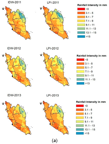
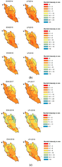
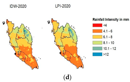
Figure 1. (a) Comparison of Annual Rainfall Intensity in mm using IDW and LPI methods with the ArcGIS Map during 2011–2013. (b) Comparison of Annual Rainfall Intensity in mm using IDW and LPI methods with the ArcGIS Map during 2014–2016. (c) Comparison of Annual Rainfall Intensity in mm using IDW and LPI methods with the ArcGIS Map during 2017–2019. (d) Comparison of Annual Rainfall Intensity in mm using IDW and LPI methods with the ArcGIS Map in 2020.

Table 1. Statistical analyses of IDW and LPI compared to ground-based rainfall data.

Year	IDW			LPI
	RMSE	MAE	R2	RMSE	MAE	R2
2011	1.64	1.16	0.65	1.55	1.12	0.69
2012	1.51	1.08	0.49	1.44	1.04	0.53
2013	1.57	1.11	0.58	1.50	1.06	0.61
2014	1.66	1.13	0.54	1.58	1.09	0.57
2015	1.31	0.91	0.35	1.25	0.88	0.39
2016	1.09	0.79	0.59	1.07	0.75	0.61
2017	1.64	1.13	0.64	1.60	1.09	0.65
2018	1.32	0.96	0.48	1.26	0.93	0.52
2019	1.40	1.06	0.47	1.33	0.99	0.52
2020	1.33	1.00	0.51	1.32	0.98	0.52

4. Conclusions

The maps of rain data were generated for each year from the year 2011 to 2020. The statistical analyses, including R², MAE, and RMSE, were implemented to test the performance of IDW and LPI as interpolation methods. In conclusion, the statistical analyses showed that the LPI method exhibited better performance than the IDW method as it had lower MAE and RMSE values but high R². In future research, the study duration can be expanded to 10 or 15 years to obtain more reliable data and reduce performance errors. In addition, a variety of widely used methodologies, such as triple collocation analysis, which does not require real values, could be proposed for more accurate study.

References

- Ceron, W.L.; Andreolo, R.V.; Kayano, M.T.; Canchal, T.; Carvajal-Escobar, Y.; Souza, R.A.F. Comparison of spatial interpolation methods for annual and seasonal rainfall in two hotspots of biodiversity in South America. An. Acad. Bras.Ciên. 2021, 93, 1–22. [Google Scholar] [CrossRef] [PubMed]
- De Silva, R.P.; Dayawansa, N.D.K.; Ratnasiri, M.D. A comparison of methods used in estimating missing rainfall data. J. Agric. Sci. 2007, 3, 101–108. [Google Scholar] [CrossRef]
- Keblouti, M.; Ouerdachi, L.; Boutaghane, H. Spatial Interpolation of Annual Precipitation in Annaba-Algeria—Comparison and Evaluation of Methods. Energy Procedia 2012, 18, 468–475. [Google Scholar] [CrossRef]
- Ahrens, B. Distance in spatial interpolation of daily rain gauge data. Hydrol. Earth Syst. Sci. 2006, 10, 197–208. [Google Scholar] [CrossRef]
- Jamaludin, S.; Sayang Mohd, D.; Wan, W.Z.; Abdul Aziz, J. Trends in peninsular Malaysia rainfall data during the southwest monsoon and northeast monsoon seasons: 1975–2004. Sains Malays. 2021, 39, 533–542. [Google Scholar]
- Tanjung, M.; Syahreza, S.; Rusdi, M. Comparison of interpolation methods based on Geographic Information System (GIS) in the spatial distribution of seawater intrusion. J. Nat. 2020, 20, 24–30. [Google Scholar] [CrossRef]
- Liang, J.; Tan, M.L.; Hawcroft, M.; Catto, J.L.; Hodges, K.L.; Haywood, J.M. Monsoonal precipitation over Peninsular Malaysia in the CMIP6 HighResMIP experiments: The role of model resolution. Clim. Dyn. 2021, 1432, 1–23. [Google Scholar] [CrossRef]
- Burrough, P.A.; McDonnell, R.A.; Lloyd, C.D. Principles of Geographical Information Systems, 3rd ed.; Oxford University Press: Oxford, UK, 2015. [Google Scholar]
- Burhanuddin, S.N.Z.A.; Deni, S.M.; Ramli, N.M. Imputation of Missing Rainfall Data Using Revised Normal Ratio Method. Adv. Sci. Lett. 2017, 23, 10981–10985. [Google Scholar] [CrossRef]
- Chow, C.W.; Cooper, J.C.; Waller, W.S. Participative Budgeting: Effects of a Truth-Inducing Pay Scheme and Information Asymmetry on Slack and Performance. Account. Rev. 1988, 63, 111–122. [Google Scholar]
- Li, J.; Heap, A.D. Spatial interpolation methods applied in the environmental sciences: A review. Environ. Model. Softw. 2014, 53, 173–189. [Google Scholar] [CrossRef]
Disclaimer/Publisher’s Note: The statements, opinions and data contained in all publications are solely those of the individual author(s) and contributor(s) and not of MDPI and/or the editor(s). MDPI and/or the editor(s) disclaim responsibility for any injury to people or property resulting from any ideas, methods, instructions or products referred to in the content. |
© 2023 by the authors. Licensee MDPI, Basel, Switzerland. This article is an open access article distributed under the terms and conditions of the Creative Commons Attribution (CC BY) license (https://creativecommons.org/licenses/by/4.0/).