Hourly Load Curves Disaggregated by Type of Consumer Using A Density-Based Spatial Clustering Technique

Carlos Andrés Peñaloza; Patricia Elizabeth Otero-Valladares

doi:10.3390/engproc2023047023

and

Department of Electrical Energy, Escuela Politécnica Nacional, Quito 170525, Ecuador

^*

Author to whom correspondence should be addressed.

^†

Presented at the XXXI Conference on Electrical and Electronic Engineering, Quito, Ecuador, 29 November–1 December 2023.

Eng. Proc.2023, 47(1), 23;https://doi.org/10.3390/engproc2023047023

This article belongs to the Proceedings XXXI Conference on Electrical and Electronic Engineering

Version Notes

Order Reprints

Abstract

This paper discusses the innovative application of a new methodology for acquiring load curves in energy systems such as Azogues Electric Company (EEA). The proposed approach imports the database from Excel and, through an iterative clustering algorithm based on density with noise, generates daily load curves with a breakdown of weekdays and weekends, identifying one curve by type of consumer. Moreover, the groups obtained are validated by means of a Silhouette verification index (IS) identifying bad groupings, which are discarded to obtain results. Per unit value responses are presented through tables with hourly values on weekdays and weekends. The graphical comparison with the previous methodology of real measurements in Excel is also added.

Keywords:

load curves; type of consumer; clustering algorithm; verification index

1. Introduction

Electric companies carry out studies in the distribution system periodically to identify and execute the necessary investments in infrastructure, with the aim of reducing technical losses and maintaining quality standards [1]. These studies involve handling various data from low voltage measurements and measurements at the feeder’s head to develop electrical studies as load characterization and support the system operator. Certain measured data may present great similarity or homogeneity, so they are analyzed in daily load curves 0–23 h.

Currently, the Excel tool is used with average or average calculations to obtain load curves by consumption group [1], but there are negative and zero value measurements that modify the final shape of the group of curves, requiring previous work to manually cluster the load curves, eliminating atypical measurement. For this reason, it is worth having an algorithm based on data mining techniques to obtain one load curve broken down by each type of consumer and use them as the starting point for expansion planning and loss calculations at medium and low voltage levels [2].

Nowadays, clustering algorithms are used in data mining tools to identify important patterns and similar distributions in large information databases. There are some methods for obtaining groups or clusters that use averages, dendrograms, and grids, but the one chosen in this work is the method based on densities that identify groups with arbitrary shapes in the presence of atypical data or noise [3].

2. Materials and Methods

2.1. Meter Measurement Data

The 236 m with measurement data are obtained from the main feeders of the EEA distribution subsystem, as well as from users connected to the secondary circuits in the years 2018 and 2019. These meters are classified by type of consumer in the cadaster of users for the EEA. Therefore, Table 1 shows the description of meters and their voltage level. Low voltage meters measure in a 220 V grid, while de medium voltage meters are located in a 13.8 kV grid. The total values for each type of consumer are shown in the right column.

Table 1. Meter information by type of consumer.

2.2. Per unit System of Data

The real daily values of average power obtained from the meter are normalized, taking as the base power the maximum on each day and in the upper part the measured data in a per unit system (pu) of 24 h (0–23 h). This is represented in Equation (1):

P_{p u} = \frac{P r o m e d i o P}{P_{m a x P o r D i a}}

(1)

$P_{p u}$ : Dimensionless value in per unit system.
$P r o m e d i o P$ : Average value of active power in kW.
$P_{m a x P o r D i a}$ : Maximum value of active power in kW per day.

2.3. DBSCAN in MATLAB

Two types of characteristic load curves are grouped according to the day of the week, a group from Monday to Friday and another from Saturdays to Sundays. Also, the types of consumers are identified as residential, commercial, industrial, and others.

In this process, the KNNsearch function is used to find a k-distances graphic of the curves; then the knee_pt function is used to find the knee of this graphic, that is, the value of Eps and its typical zone, which is a necessary argument to establish the clusters in the DBSCAN function. The Mpts argument is set to a relatively low value so that all points belonging to the same group are included. This algorithm requires three input parameters and returns an idx vector with the resulting grouping or cluster. Next, Equation (2) in MATLAB R2021b:

i d x = D B S C A N (X, E p s, M p t s)

(2)

$X$ : Size of the neighbor list or data matrix.
$E p s$ : Radius that delimits the neighborhood area of a point (neighborhood-Eps).
$M p t s$ : Minimum number of data or objects around neighborhood-Eps.

2.4. KNNSearch

This function finds the K nearest neighbors, according to Euclidean distances, and returns their indices in a column vector d and their respective distances kD. It uses input data or a database. Equation (3) shows its structure in MATLAB R2021b for its correct use.

[d, k D] = k n n s e a r c h (X, Y, N a m e, V a l u e)

(3)

$X$ : Values in pu of data 0–23 h for the measurement days.
$Y$ : Values in pu 0–23 h.
$N a m e$ : Write “K” and calculate the nearest neighbor distances.
$V a l u e$ : Matrix size of how many nearest neighbors in the distance metric.

2.5. Kneepoint

The kneepoint function advances along the K-dist plot of distances, one bisection point at a time, fitting two lines, these being the first derivative and the second derivative. The knee is at a bisection or threshold point that minimizes the sum of errors for the two adjustments. Any value less than this threshold density Eps can efficiently cluster patterns because these would lie in typical k-dist plot territory [4]. Equation (4) in MATLAB:

x = k n e e_p t (d i s t a n c e s)

(4)

$d i s t a n c e s$ : Euclidean distances of the K-dist graph.
$x$ : Value in x of the elbow of the K-dist type graph.

2.6. Validation Index Silhouette (IS)

Each group can be represented by a silhouette, which is based on the comparison of their closeness and separation. This silhouette shows which objects are well classified within their group and which are simply infiltrating between the groups. The average width of the silhouette provides an assessment of clustering validity and could be used to select an “appropriate” number of clusters [5]. Equation (5) in MATLAB:

s = s i l h o u e t t e (X, i d x)

(5)

$X$ : Data between objects.
$i d x$ : is the partition obtained (by applying some grouping or cluster technique).
$s$ : Value between −1 and 1, denoting 1 as belonging to the cluster and −1 not belonging.

3. Discussion

3.1. Clustering on Weekdays and Weekends

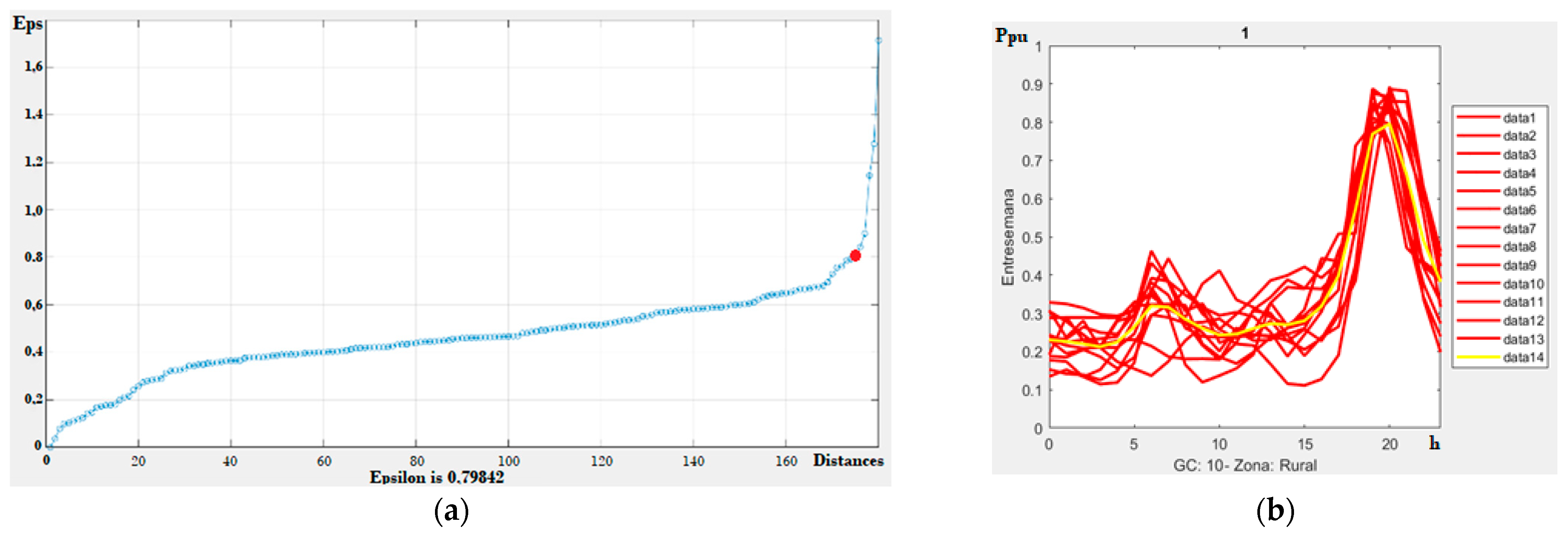
Figure 1a is a K-dist type graph made to find Epsilon (Eps) with the function Kneepoint. The respective knee of the function of distances is denoted with a red circle and any point up to that curve will represent a correct value to use it as an entry parameter in DBSCAN. Eps is established with the kneepoint function, and Mpts is set to a value greater than 1. Groupings such as the one in Figure 1b begin to be obtained, which contain descriptions on the bottom, top, and lateral sides.

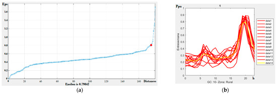
Figure 1. Complementary algorithms and clustering (a) Kneepoint and Knnsearch on finding Eps (b) Partial result of a residential group in the clustering algorithm.

Then, Figure 2a shows the grouping of meters considered noise. Given the amount of data in this figure, a similar behavior is not distinguished in the characteristic curves, and a resulting yellow curve is also observed, which is not entirely true for this grouping. Then, the algorithm validates the grouping performance. For this task, the index IS, shown in Figure 2b, is the verification in MATLAB and detects which cluster is incorrectly grouped, having index values of −1.

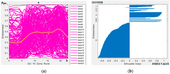
Figure 2. Noise and validation (a) Cluster 8 on weekdays NOISE; (b) SILHOUETTE validation index, identifying cluster 8 as noise.

The same procedure is applied for the weekends, obtaining different values on the kneepoint, the grouping, and the validation. It is important to mention that noise is treated again with filters that take the eliminated curves and apply the clustering technique to obtain even more results from the system.

3.2. System Results

After submitting the database to the algorithm proposed in MATLAB R2021b, load curves for weekdays and weekends were found. The objective is to establish only one curve per type of consumer and a system curve. For this, reference [6] is used. Figure 3 shows the characteristic curves of the different consumption groups and a total curve of the system, having in the x-axis the hour of the day 0–23 h and in the y-axis the per unit value of the measurement.

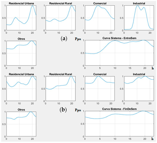
Figure 3. Graphical results in

P_{p u}

of each consumer and system curve. (a) Weekdays, (b) Weekends.

Table 2 presents the numerical results of the curves shown in Figure 3, they are separated in weekdays to the left side and the clustering results for weekends on the right.

Table 2. Load curves numerical results imported from MATLAB (a) weekdays; (b) weekends.

3.3. Comparison with Previous Method

The method of obtaining load curves used by the EEA focuses on using the real measurements, exporting them to an Excel file, and then, with a series of filters on georeferencing, voltage level, or feeders, obtaining similar curves in real values of Active Power kWh. Then, empirically, eliminates curves that do not represent a characteristic behavior of the type of consumer to finally group and obtain the average of the similar curves. These curves are later used in distribution network simulation programs and must be in pu to obtain electrical analysis results, power flows, and losses.

Weekdays Comparison

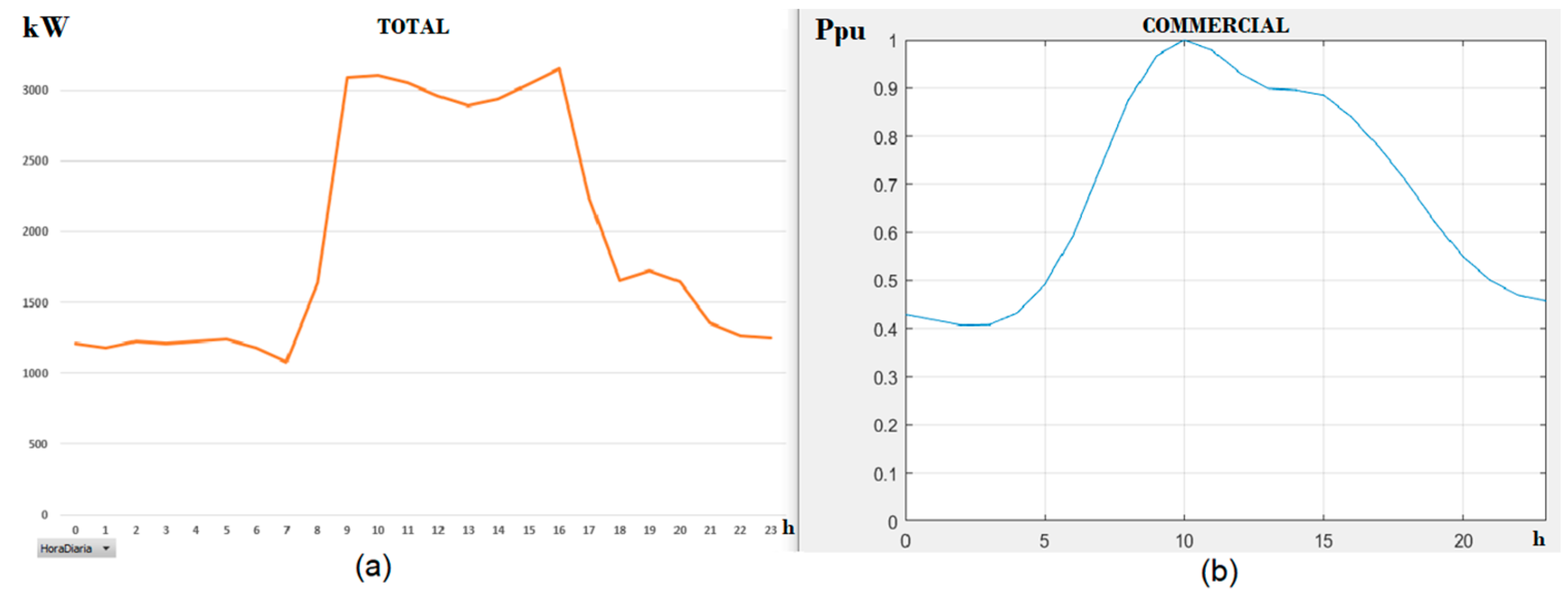
Figure 4 and Figure 5 show the final curve during the weekdays where the left side is the result with the previous method of the electric company in Excel, while the right side shows the resulting curve obtained with the DBSCAN algorithm in Matlab. In addition, the new method changes the y-axis from real value in kW to pu values while it maintains the x-axis in daily hours.

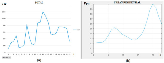
Figure 4. Final load curve on weekdays Urban residential. (a) Previous method; (b) DBSCAN.

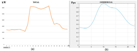
Figure 5. Final load curve on weekdays Commercial. (a) Previous method; (b) DBSCAN.

The previous curves indicate different behavior for the same type of Urban Residential consumers, and the peaks are given in other hourly values. This is because in the old method, there is a lack of data to carry out filters in Excel, while the new one provides the direct grouping of similar curves with the density algorithm.

Figure 5 exhibits similar results at consumption peaks. This time, the database in Excel included many similar curves for the commercial consumer, and the grouping step was successful. In the same way, the values in pu are convenient for better identification of the resulting curve and its maximum demand.

4. Conclusions

The advantage of the method presented in this written work is the use of a clustering algorithm to obtain load curves in pu and the validation tool to discard atypical measurements. These two advantages outperform the previous EEA methodology by obtaining only one curve by type of consumer using a clustering technique instead of considering the analyst experiences.

During the clustering procedure, load curves that have the behavior of public lighting or industries that only operate in the early morning hours or at night were identified by the noise application of the algorithm. These types of consumers did not enter the obtaining of final curves due to their little intervention in the distribution electrical system.

Author Contributions

Conceptualization, P.E.O.-V. and C.A.P.; methodology, C.A.P.; software, C.A.P.; validation, C.A.P., P.E.O.-V.; formal analysis, P.E.O.-V.; investigation, C.A.P.; data curation, C.A.P.; writing—original draft preparation, C.A.P.; writing—review and editing, P.E.O.-V.; visualization, P.E.O.-V.; supervision, P.E.O.-V.; project administration, P.E.O.-V.; All authors have read and agreed to the published version of the manuscript.

Funding

This research received no external funding.

Institutional Review Board Statement

Not applicable.

Informed Consent Statement

Informed consent was obtained from all subjects involved in the study.

Data Availability Statement

Data is unavailable due to privacy restrictions.

Conflicts of Interest

The authors declare no conflict of interest.

References

Ministerio de Electricidad y Energías Naturales No Renovables, “Plan Maestro de Electricidad 2018–2027”, Chapter 3, Estudio de la Demanda. Available online: https://www.recursosyenergia.gob.ec/plan-maestro-de-electricidad/ (accessed on 13 March 2023).
ARCONEL. Plan Maestro de Electrificación 2013–2022, Perspectiva y Expansión del Sistema Eléctrico Ecuatoriano. Available online: https://www.regulacionelectrica.gob.ec/plan-maestro-de-electrificacion-2013-2022/ (accessed on 15 April 2023).
Fong, S.; Rehman, S.U. DBSCAN: Past, Present and future. In Proceedings of the Fifth International Conference on the Applications of Digital Information and Web Technologies (ICADIWT 2014), Chennai, India, 17–19 February 2014. [Google Scholar]
Irwin, D.; Albrecht, J.; Satopa, V. Finding a “Kneedle” in a Haystack: Detecting Knee Points in System Behavior. In Proceedings of the 31st International Conference on Distributed Computing Systems Workshops, Minneapolis, MN, USA, 20–24 June 2011. [Google Scholar]
Rousseeuw, P.J. Silhouettes: A graphical aid to the interpretation and validation of cluster analysis. J. Comput. Appl. Math. 1999, 20, 53–65. [Google Scholar] [CrossRef]
Gönen, T. Electric Power Distribution Engineering; CRC Press: Boca Raton, FL, USA, 2014. [Google Scholar]

Figure 1. Complementary algorithms and clustering (a) Kneepoint and Knnsearch on finding Eps (b) Partial result of a residential group in the clustering algorithm.

Figure 2. Noise and validation (a) Cluster 8 on weekdays NOISE; (b) SILHOUETTE validation index, identifying cluster 8 as noise.

Figure 3. Graphical results in

P_{p u}

of each consumer and system curve. (a) Weekdays, (b) Weekends.

Figure 4. Final load curve on weekdays Urban residential. (a) Previous method; (b) DBSCAN.

Figure 5. Final load curve on weekdays Commercial. (a) Previous method; (b) DBSCAN.

Table 1. Meter information by type of consumer.

Type of Consumer	Low Voltage 220 V	Medium Voltage 13.8 kV	Total
Commercial	25	20	45
Industrial	18	14	32
Others	9	9	18
Residential	131	0	131
No Identified	5	5	10
Total	188	48	236

Table 2. Load curves numerical results imported from MATLAB (a) weekdays; (b) weekends.

(a) weekdays
Daily Hour	Residential U	Residential R	Commercial	Industrial	Others	System Curve-Weekdays
0	0.2295	0.4077	0.4293	0.0369	0.6848	0.4910
1	0.2234	0.3907	0.4179	0.0363	0.6836	0.4810
2	0.2166	0.3690	0.4070	0.0360	0.6790	0.4689
3	0.2203	0.3577	0.4083	0.0372	0.6730	0.4658
4	0.2592	0.3706	0.4330	0.0411	0.6695	0.4869
5	0.3544	0.4089	0.4916	0.0524	0.6723	0.5435
6	0.4687	0.4478	0.5940	0.1105	0.6973	0.6365
7	0.5211	0.4553	0.7355	0.2970	0.7510	0.7578
8	0.4886	0.4338	0.8741	0.6037	0.8016	0.8791
9	0.4213	0.4020	0.9673	0.8748	0.8257	0.9586
10	0.3743	0.3749	1.0000	1.0000	0.8305	0.9829
11	0.3463	0.3649	0.9785	0.9806	0.8287	0.9607
12	0.3098	0.3726	0.9308	0.8761	0.8245	0.9099
13	0.2718	0.3909	0.8990	0.8071	0.8219	0.8761
14	0.2661	0.4143	0.8957	0.8488	0.8245	0.8922
15	0.3017	0.4465	0.8853	0.9244	0.8312	0.9305
16	0.3647	0.4969	0.8404	0.8927	0.8480	0.9453
17	0.4668	0.5931	0.7768	0.6857	0.8909	0.9372
18	0.6531	0.7578	0.7039	0.3999	0.9550	0.9526
19	0.8800	0.9303	0.6224	0.1884	1.0000	0.9942
20	1.0000	1.0000	0.5499	0.0934	0.9988	1.0000
21	0.9326	0.9422	0.4998	0.0625	0.9487	0.9296
22	0.7421	0.8288	0.4698	0.0517	0.8692	0.8131
23	0.5992	0.7542	0.4571	0.0476	0.8148	0.7339
(b) weekends
Daily Hour	Residential U	Residential R	Commercial	Industrial	Others	System Curve-Weekends
0	0.7927	0.5184	0.7238	0.7468	0.7484	0.7648
1	0.7219	0.5000	0.7206	0.7263	0.7454	0.7397
2	0.6370	0.4811	0.7157	0.7064	0.7401	0.7107
3	0.5861	0.4721	0.7115	0.7083	0.7351	0.6961
4	0.5732	0.4762	0.7121	0.7213	0.7233	0.6945
5	0.5842	0.4936	0.7195	0.7379	0.6984	0.7005
6	0.6141	0.5212	0.7385	0.7494	0.6853	0.7168
7	0.6598	0.5554	0.7867	0.7726	0.7129	0.7555
8	0.7203	0.5941	0.8722	0.8246	0.7563	0.8162
9	0.7689	0.6157	0.9593	0.8731	0.7767	0.8652
10	0.7579	0.6118	1.0000	0.9177	0.7750	0.8801
11	0.7140	0.6155	0.9901	0.9538	0.7702	0.8760
12	0.6959	0.6265	0.9531	0.9438	0.7722	0.8647
13	0.6944	0.6290	0.9091	0.9199	0.7798	0.8519
14	0.6704	0.6347	0.8653	0.9420	0.7888	0.8452
15	0.6497	0.6425	0.8223	0.9834	0.8039	0.8453
16	0.6661	0.6558	0.7814	1.0000	0.8397	0.8542
17	0.7262	0.7342	0.7578	0.9952	0.9103	0.8934
18	0.8355	0.8788	0.7555	0.9549	0.9839	0.9551
19	0.9500	0.9916	0.7555	0.9188	1.0000	1.0000
20	1.0000	1.0000	0.7485	0.8959	0.9585	0.9972
21	0.9745	0.9164	0.7398	0.8728	0.8937	0.9526
22	0.8981	0.7987	0.7341	0.8659	0.8272	0.8935
23	0.8380	0.7223	0.7322	0.8689	0.7893	0.8559

Disclaimer/Publisher’s Note: The statements, opinions and data contained in all publications are solely those of the individual author(s) and contributor(s) and not of MDPI and/or the editor(s). MDPI and/or the editor(s) disclaim responsibility for any injury to people or property resulting from any ideas, methods, instructions or products referred to in the content.

© 2023 by the authors. Licensee MDPI, Basel, Switzerland. This article is an open access article distributed under the terms and conditions of the Creative Commons Attribution (CC BY) license (https://creativecommons.org/licenses/by/4.0/).

Hourly Load Curves Disaggregated by Type of Consumer Using A Density-Based Spatial Clustering Technique^†

Abstract

1. Introduction