Abstract
A problem with applying machine learning for analyzing power system dynamics is the lack of specific datasets. In this realm, defining a strong methodology to obtain power system dynamic data is an important task prior to the application of any machine learning tool. This is particularly important considering the current growing research in the field of self-healing grids. Thus, this paper presents a well-defined stochastic methodology that can be used to generate dynamic data that can afterwards be analyzed using machine learning tools. The proposed method is based on a Monte Carlo simulation and this paper presents the procedure to perform it.
1. Introduction
Traditionally, power system security assessments have been studied using deterministic methodologies, which consider some extreme operating conditions (different load levels) and selected critical contingencies (associated with some fault types and fault locations). This type of study ignores the stochastic or probabilistic nature of real power systems, and therefore certain severe events that could lead a system to potential insecure conditions may be ignored [1]. Since the huge volume of uncertainties greatly influences the power system dynamic response, it is necessary to apply mathematical tools which allow for the consideration of the most probable scenarios. One of the main classes of probabilistic techniques is the Monte Carlo (MC)-based simulation, which provides the possibility of obtaining more realistic results, mainly for complex system analysis [1,2], since it avoids using surrogate models. The MC method allows for simulating phenomena with significant involved levels of uncertainty, which correspond to electric power systems’ operational conditions. In addition to the previously stated fact, the recent spike of interest in machine learning and artificial intelligence (AI) methods that can be applied to power system dynamics has given rise to a major issue for scholars and scientists: how to objectively compare the machine learning and data mining schemes and algorithms for stability prediction (i.e., classification or regression)? [3,4,5,6]. This problem has generated even more interest with the recent design of smart grid applications to perform timely self-healing and adaptive reconfiguration actions based on system-wide analysis, with the objective of reducing the risk of power system blackouts. A real-time dynamic vulnerability assessment (DVA) must be performed to decide and coordinate the appropriate corrective control actions, depending on an event’s evolution [3,4]. For this aim, the application of machine learning and AI tools constitutes a very attractive alternative. Thus, emerging technologies such as phasor measurement units (PMUs) and wide area monitoring systems (WAMSs) offer a new benchmark for performing post-contingency DVAs that could be used to trigger system integrity protection schemes (SIPSs) or activate wide area controls to implement enhanced corrective control actions [3,4,5,6]. In connection to this, the fast detection of critical conditions (from the shortest possible data record prior to, during and after a fault) is instrumental in response-based special stability controls. Such a scheme should be as agnostic as possible to the type of instability that may occur within, say, 5 to 10 s after the fault clearing or the triggering event. Therefore, accurate and fair tests need to be conducted to determine the specific tool behavior. Nevertheless, the problem found in the recent literature is that most authors that are performing research on this important topic do not have specific datasets to test their models in such a way to obtain fair comparisons. In this vein, especially since the emergence of deep learning, they claim that they have “the best algorithm” ever, in terms of accuracy and pre-emption time. However, while authors have used well-known test systems, the dataset is never the same, and one of the reasons for this is the lack of a well-defined methodology for data generation. Thus, it is becoming more and more difficult to separate well-founded claims from fake claims and erroneous claims that have been made in good faith by authors. Based on the mentioned problem, this paper presents a well-defined stochastic methodology that can be used to generate sufficiently confident dynamic data that can be used for DVA applications based on machine learning. The method is based on Monte Carlo simulations, which are stochastic processes that are commonly used to perform probabilistic assessments. For instance, a Monte Carlo simulation is used in [7] to emulate the effect of high-speed wind on a test system and determine the failure state of a transmission using a reduced fragility function that was proposed to evaluate the resilience of the system. Also, a Monte Carlo simulation was combined with k-means clustering and an elbow plot to determine feasible scenarios of photovoltaic and wind generation integration into the power system in [8] for solving the probabilistic optimal power flow problem. A Monte Carlo simulation is also used in [9] to simulate the vehicle to grid (V2G) systems, including the process of power flow and the battery state, for charging and discharging (SoC) electric vehicles (EVs). However, the use of Monte Carlo simulations for power system dynamic data generation oriented to DVAs has not been explored in these works.
Therefore, the main objective of applying a Monte Carlo simulation in this paper is to generate post-contingency system static or dynamic data considering a great number of the probable scenarios and contingencies, even those that could push the system to potential cascading events and subsequent blackouts. Then, the number of MC repetitions cannot be directly determined by the convergence relations (such as those presented in [2]). Thus, the number of iterations will depend on the complexity of the system and the attainment of a dataset that is sufficiently representative to reveal post-contingency system vulnerability patterns and statuses. In connection to this, it is suggested that the number of generated vulnerable cases represents at least 20% of the total number of cases. This value has been empirically determined through several experiments that were carried out during the development of the present research.
The rest of the paper is organized as follows: Section 2 describes the concept of Monte Carlo simulations. In Section 3, the general procedure to perform a Monte Carlo simulation for power system dynamic data generation oriented to DVAs is presented. Section 4 provides numerical results to demonstrate the feasibility and performance of the proposal applied to different machine-learning-based DVA methods. Finally, a discussion of the proposed approach as well as the conclusions and outlook for future research are summarized in Section 5.
2. Monte Carlo Method as a Data Generation Technique
The Monte Carlo method is a repetitive procedure that consists of evaluating, at each repetition, the system response through the uncertainty function h, using a set of input variables (z) which are generated randomly from their probability distribution functions (PDFs), in order to obtain numerical random output values (v) [2].
Thus, the several MC outputs (i.e., one output per iteration) are usually aggregated in order to obtain statistical results (typically represented by the expected value and standard deviation) [1,2]. However, this paper does not specifically apply MC-based simulations with the aim of obtaining statistical information. The main objective of using this probabilistic technique is to generate post-contingency system static or dynamic data considering a great number of the probable scenarios and contingencies, even those that could push the system to potential cascading events and subsequent blackouts.
3. Materials and Methods
To perform MC-based simulations, several input data are required. These data depend on the objective of the simulation, and they are usually represented by their corresponding probability distribution functions (PDFs). For the proposed objective, the probabilistic models of power system random variables, as well as the grid topology, are structured for a short-term planning horizon to reflect the behavior of the system as realistically as possible [2]. In connection to this, the basic data to be considered in the MC-based simulation, which must be previously prepared by the system operator, are the short-term forecasting of nodal loads, the short-term unit commitment, the short-term system topology, and the random generation of N-1 contingencies.
3.1. Short-Term Forecasting of Nodal Loads
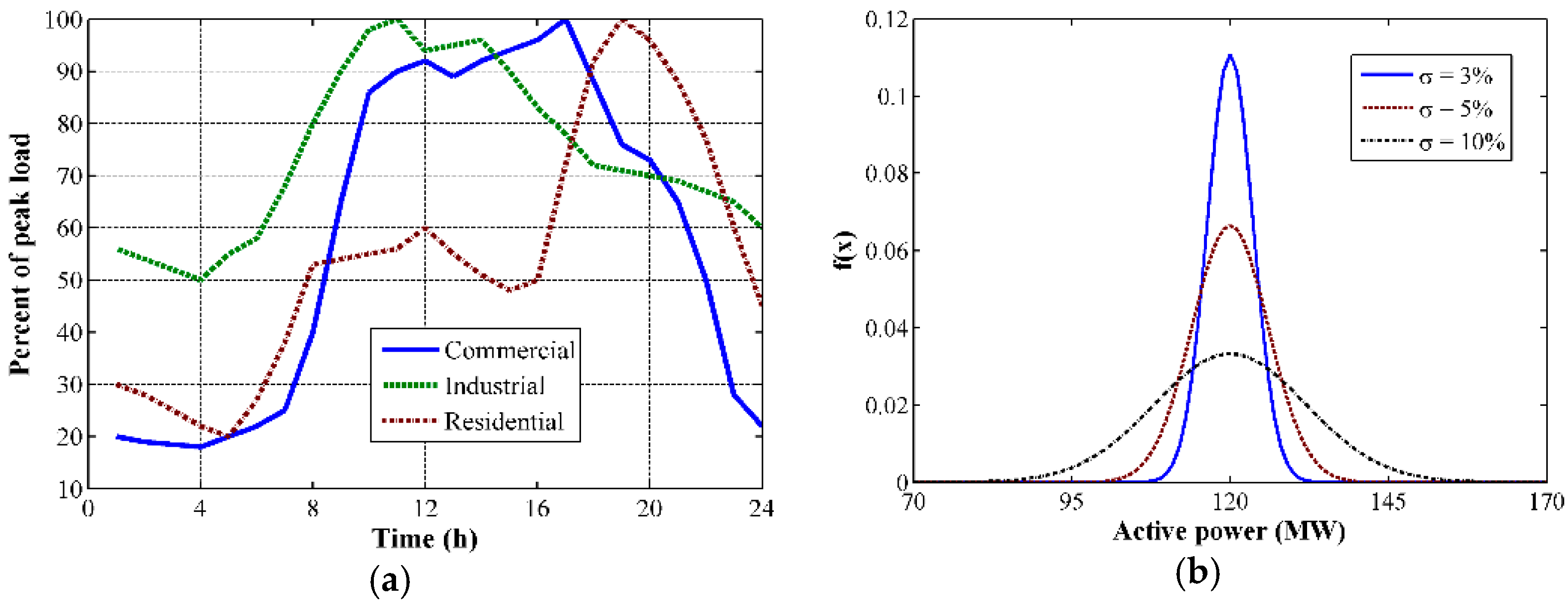
Electric power demand and energy consumption correspond to non-linear time functions that present different values in each grid load node. This peculiarity is because of the nature and diversity of customers (i.e., residential, commercial or industrial). In connection to this, the hourly behavior of each load (load chronology) is characterized by different daily load curves which resemble customers’ own usage of electricity [10]. Therefore, the analysis of load forecasting must reflect this behavior in each of the nodal loads. Another aspect to be considered is the horizon of operational planning. There are three types of operational planning horizons: long-term, mid-term, and short-term [2,10]. Short-term load forecasting is one of the operator’s common tasks due to it being employed as an input of the short-term economic dispatch. Since the horizon of interest for dynamic analysis is limited to the short term, which embraces a forecasting timeframe of one day to several weeks [10], three different daily load curves (i.e., typical residential, typical industrial and typical commercial) can be used. These typical load curves represent the results of the corresponding short-term load forecasting performed by the ISO. Figure 1a illustrates the load curves for various end-user classes, which can be used as nodal loads in test power systems for generating dynamic data. It is worth mentioning that whilst the active power demand is determined based on the daily load curves depicted in Figure 1a, the reactive power demand will be estimated based on the assumption that the power factor keeps a quasi-invariant behavior. Considering that, regardless of the load forecasting method, the actual system load behavior will always differ from that obtained from forecasting; the resulting uncertain behavior of the load must be considered. Thus, the forecasting uncertainty has been included in the formation of the hourly nodal loads via normal (or Gaussian) distribution functions (2).
where μ is the mean or expectation of the distribution, σ is its standard deviation, and its variance is therefore σ2,, whereas μ is defined depending on the base case load data and the corresponding load curve of Figure 1a and σ is introduced as a pre-defined parameter (which will depend on a historically based statistical analysis in a real system). Figure 1b presents a family of the described normal PDFs with a mean of 120 MW and different values for the parameter σ.
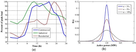
Figure 1.
Stochastic load model: (a) class-specific daily load curves and (b) the family of normal distribution functions with parameter σ.
3.2. Short-Term Unit Commitment and Short-Term System Topology
The determination of the optimal scheduling of generation units to meet the demand that is forecasted over a future short-term period is a complex operational planning problem. This problem is the so-called “unit commitment”, and it consists of economically optimizing the schedule of available generating units, subject to specific constraints [11].
There are two types of typical constraints: the “coupling” constraints and the “local” constraints [11], and both are associated with uncertainties [2]. The coupling constraints refer to the amount of required power, and their associated uncertainties are due to possible changes in the market dispatching rules and primary energy sources’ availability. Likewise, the local constraints deal with technical limitations which might influence the unit operation status (due to maintenance plans or the failure of components). Since the solution of unit commitment comprises a complex optimization problem (solved by different approaches [11]), it is assumed that this task has been previously carried out by the operator. So, there already exists a tentative short-term schedule of dispatching units, which also includes the available spinning reserve. This tentative schedule will be used as the input for the methodology proposed in this paper.
Short-term operational planning also concerns the determination of grid topology, considering all the available transmission elements and the execution of a procedure called “network topology optimization” [12]. The objective is to use the available assets to increase grid flexibility and efficiency.
3.3. Random Generation of N-1 Contingencies
The N-1 contingencies of system elements are assumed to be independent events and are generated randomly. The set of possible independent contingencies includes generator outages, load events and three-phase short circuits in transmission lines, followed by the outage of the faulted line. The short circuits are randomly applied at different locations on the transmission lines. It is worth mentioning that the possible selected contingencies might be adapted to the system under study to consider the most probable and stressful perturbations. The probability of the fault type obeys a discrete probability distribution, which depends on a system’s historical data, as shown in Equation (3) [13].
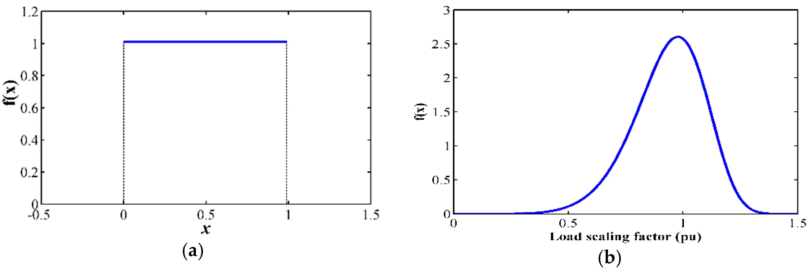
where Pi is the probability of the i-th fault type, fi is the number of the i-th fault type and M is the number of considered fault types. The probability of the fault’s location and the amount of load to be modified in each load event is determined by adequate PDFs that are also defined by historical statistical data. In test power systems, the random generation of contingencies can be based on two types of distribution functions: uniform (random faulted element selection and random short circuit location) and Weibull (random load step size). Based on the consideration that the occurrence of any contingency is equally probable (this aspect does not necessarily need to be satisfied in a real system, where the selection of the appropriate PDF will depend on statistics), the random faulted element selection is based on a uniform PDF (4). This PDF is illustrated in Figure 2a.
where a and b are the minimum and maximum values of the PDF support. In this specific application, a = 0 and b = 0.99, and the index of the selected faulted element (Elementi) is determined via Equation (5).
where x is the random variable between a and b, Nelements is the number of elements to be susceptible to failures, Elementi = 1…Nelements is the index of the selected faulted element, and floor(·) represents the rounding toward a negative infinity value. Likewise, it has been considered that all the line lengths present the same probability of being susceptible to short circuits (this fact is not necessarily satisfied in a real system, where the selection of the appropriate PDF will depend on statistics). In this connection, the random short circuit location is also based on the uniform PDF represented via Equation (4). In this case, parameters a and b are equal to 0% and 100% of the line length.
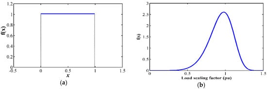
Figure 2.
Random N-1 contingencies: (a) uniform distribution function for selection of faulted element and (b) the Weibull distribution function for load events.
Finally, the Weibull distribution function has been adopted for representing the random load step size to be increased or disconnected in load events. This type of PDF has the property of being able to adapt its shape to the specific physical characteristic which, in this case, is the fact that the load can be completely disconnected (negative step of −100%), but it is practically impossible to be increased in the same percentage (positive step of 100%). Thus, whilst the negative side can vary from 0% to −100%, the positive range might only vary from 0% to a maximum value determined via the statistics in a real system. The Weibull PDF (6) can be easily adapted to represent this characteristic.
where k > 0 is the shape parameter and λ > 0 is the scale parameter of the distribution. In the proposed application, x corresponds to the load scaling factor, which can vary from 0 to infinity, and represents a factor to be multiplied by the base case load value to acquire the post-event load value. Then, the load step size (in p.u.) will be equal to x − 1. Figure 2b depicts the Weibull PDF employed for representing the load scaling factor, where λ = 1, and k = 7. Once adequate PDFs have been defined, a sampling procedure must be selected to draw the contingency random samples in consistency with their PDFs. Based on the analysis performed in [2], the random sampling technique is selected for the proposed Monte Carlo simulation due to it having shown better results in terms of the mean and variance in a power system probabilistic dynamic analysis.
3.4. General Structure of the Monte Carlo Process
Based on the previously settled system operating policies (i.e., a pre-defined short-term system topology and unit commitment dispatch rules) and the probabilistic models of the input parameters (i.e., the load variation and occurrence of contingencies), a Monte Carlo-type simulation is performed to iteratively evaluate the system responses, which would resemble those signals recorded by the PMUs in real time, with the goal of structuring a performance database.
In connection to this, and depending on the specific application, static or dynamic N-1 contingency simulations, as well as a modal analysis, are performed via the MC process, as depicted in Figure 3. First, the PDFs randomly generate the input variables to be considered in the Monte Carlo simulation, i.e., the load in each bus, the type of contingency (e.g., short circuit, generation outage or load event), the faulted element (line, generator or load), the short circuit location, the amount of load to be changed or the branch outage, in the case of static contingency analysis. Then, optimal power flow (OPF) is performed for every trial set of input variables to define feasible pre-contingency steady-state scenarios. Afterwards, an N-1 static contingency analysis, dynamic time domain simulations, or a modal analysis are performed to obtain the pre- and post-contingency power flow results, the post-contingency dynamic data or the eigenvalues and eigenvectors, respectively. These data will then be used as inputs for machine learning tools.
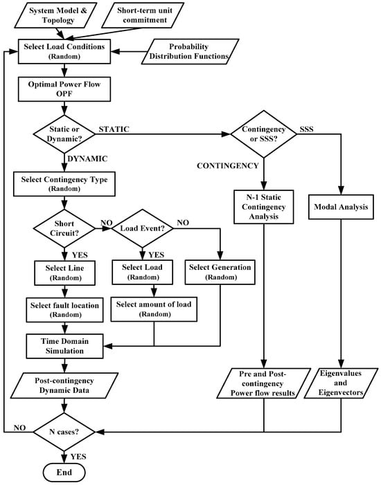
Figure 3.
Methodological framework of the proposed MC-based simulations.
4. Results
The proposed MC-based simulation has been applied to the IEEE New England 39-Bus test system [3] to obtain several post-contingency dynamic data that can later be used to train different machine learning tools for performing DVAs. In connection to this, [3,4] the data can be used to perform a DVA for five different symptoms of system stress: transient stability, oscillatory stability, short-term voltage stability, short-term frequency stability, and post-contingency overloads initiated by topological modifications and power injection changes which follow an N-1 contingency. Likewise, [5,6] show the application for generating data for transient stability assessments using machine learning.
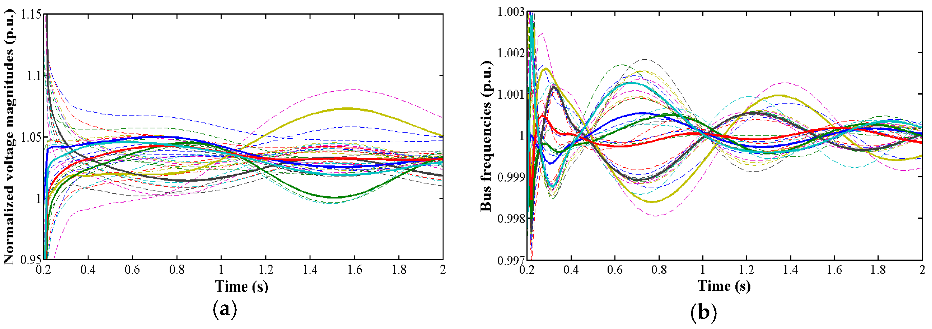
Figure 4 illustrates the bus signals (i.e., bus voltage magnitudes and frequencies) for two different Monte Carlo iterations obtained with the application of the proposed methodology.
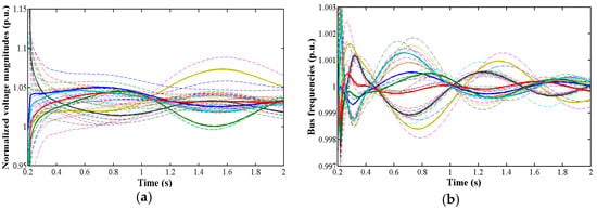
Figure 4.
Dynamic data obtained from MC-based simulation: (a) normalized voltage magnitudes: three-phase short circuit applied on lines 13–14 at 51.3% of the line length, high-load scenario; (b) bus frequencies: three-phase short circuit applied on lines 6–11 at 96.0% of the line length, medium-load scenario. Colorful dotted lines represent the different coherent areas determined in the system and solid lines show the representing centroids for each area.
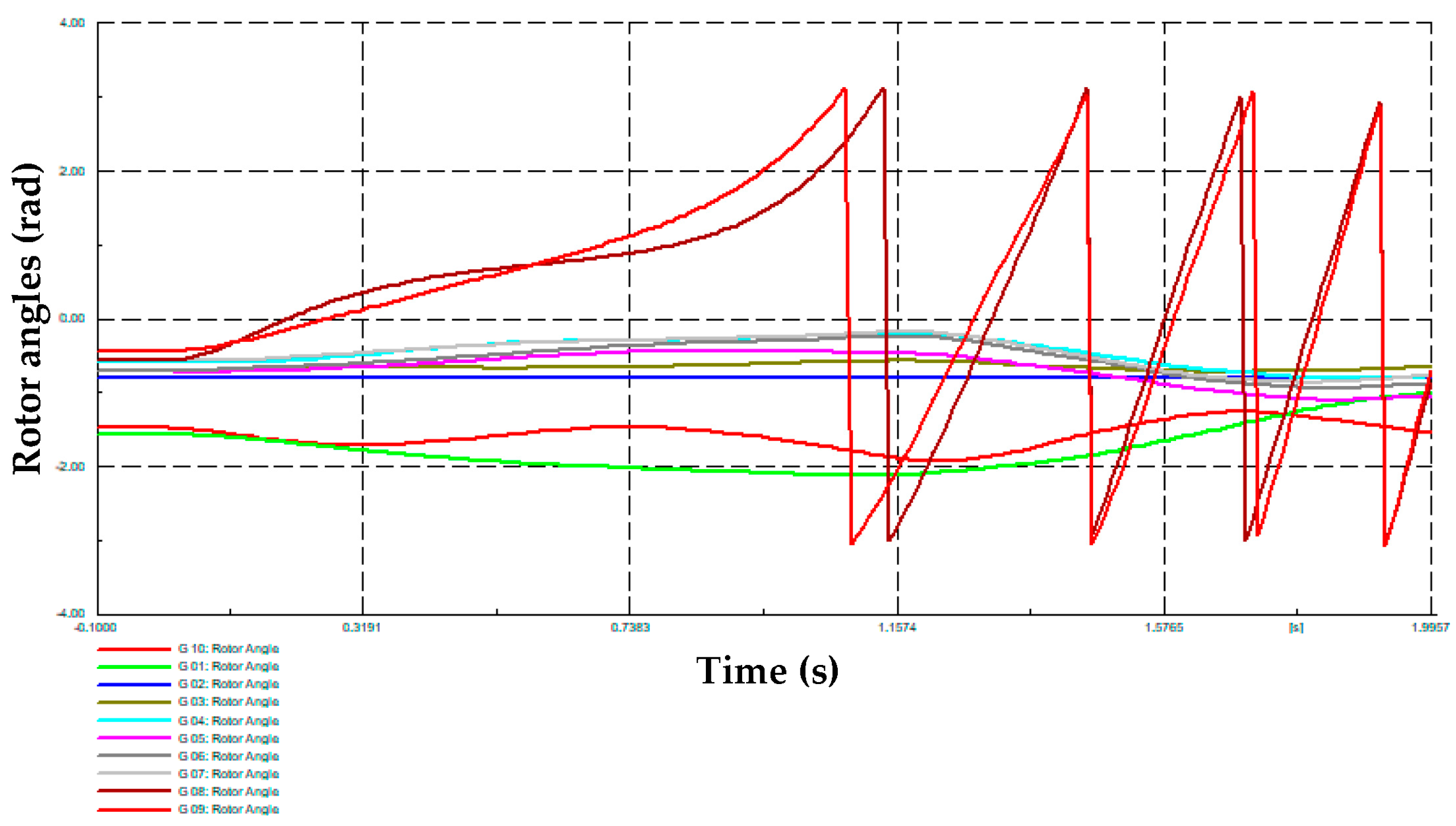
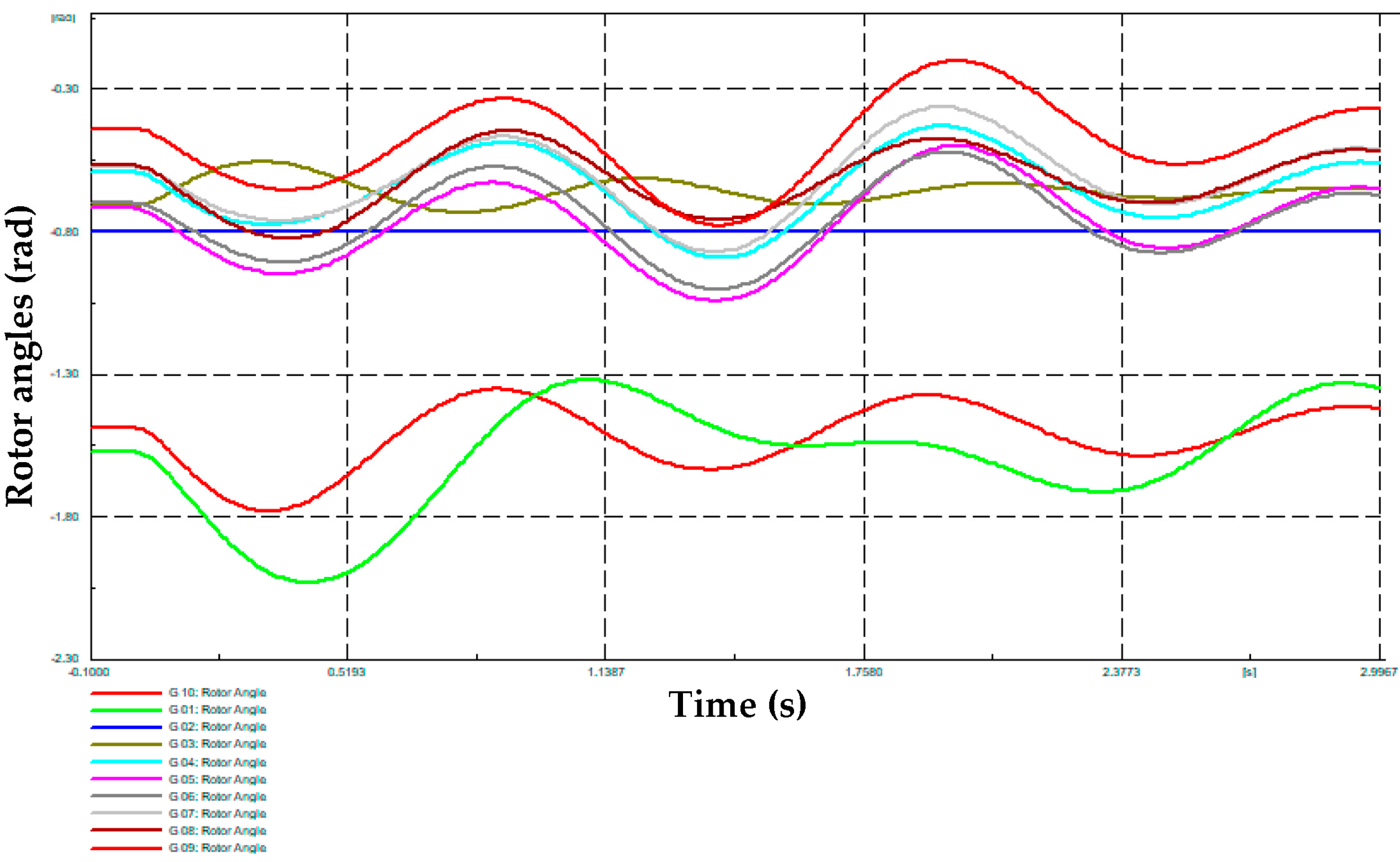
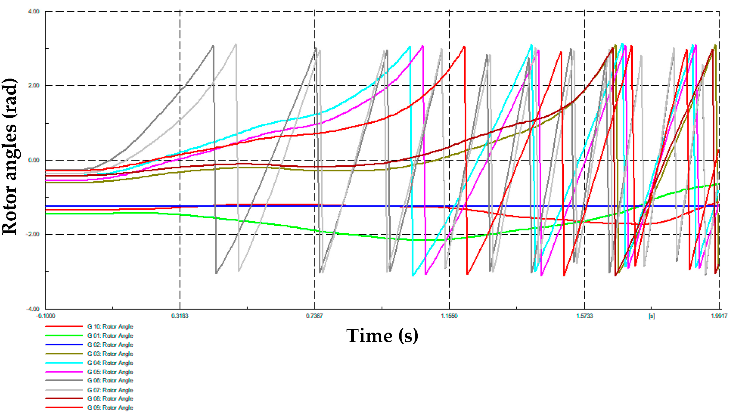
On the other hand, Table 1 presents the dynamic responses of the single machine equivalent (SIME) method used in [5] for a transient stability assessment, corresponding to three cases of the Monte Carlo simulation: “unstable”, “stable” and “very unstable”, respectively. Likewise, Figure 5, Figure 6 and Figure 7 present the rotor angles of synchronous generators for each one of these cases. It is possible to observe how the proposed MC simulation can determine possible cases with different stability statuses, which is important for training machine learning tools for system security assessments.

Table 1.
MC-based SIME simulation results.
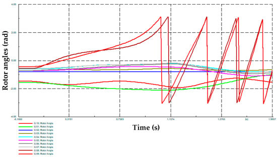
Figure 5.
Synchronous machines’ rotor angles obtained from the MC-based simulation—unstable case.
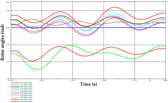
Figure 6.
Synchronous machines’ rotor angles obtained from the MC-based simulation—stable case.
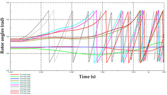
Figure 7.
Synchronous machines’ rotor angles obtained from the MC-based simulation—very unstable case.
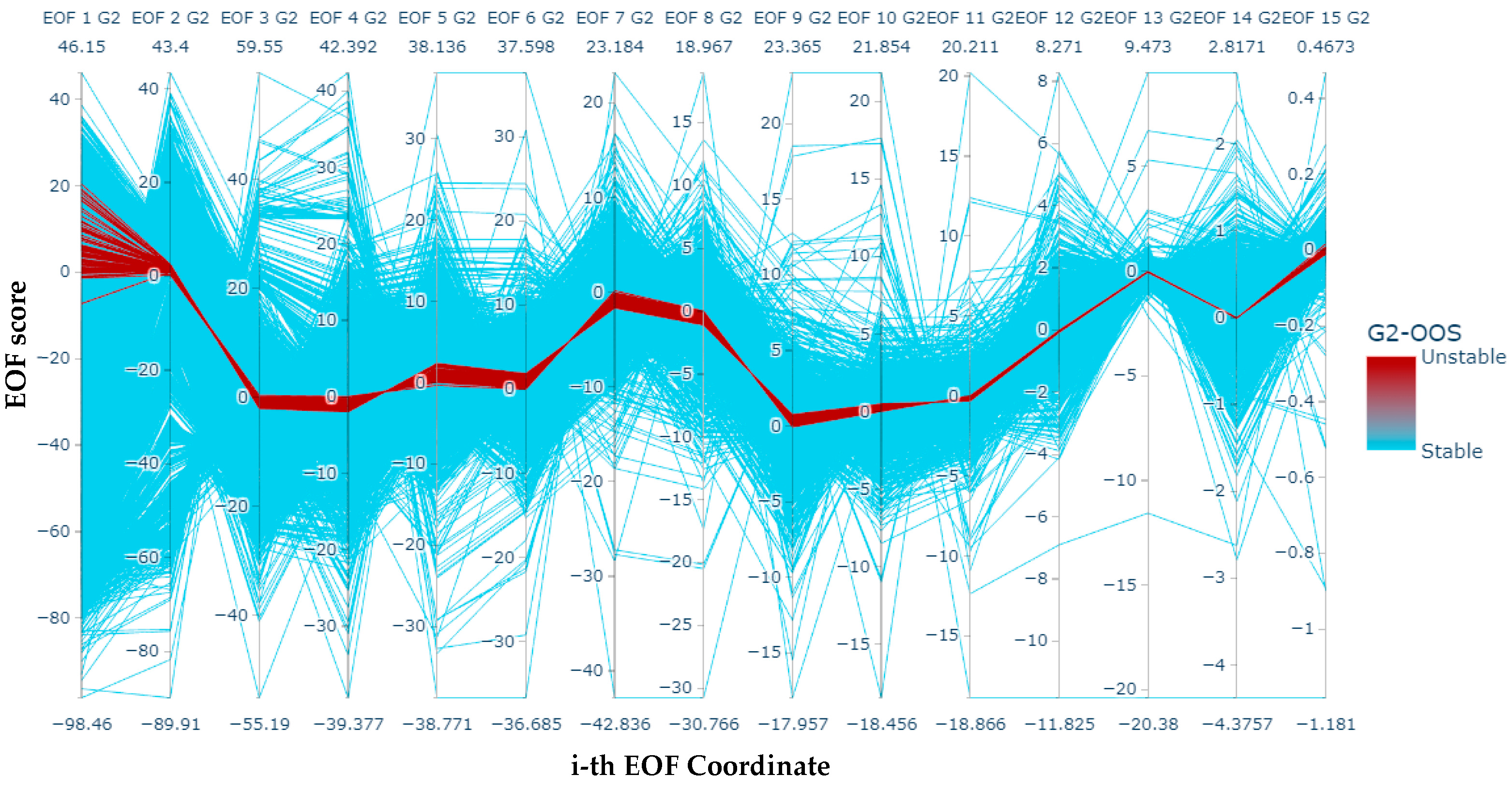
Finally, with the aim of appreciating how the MC-based dynamic data are capable of being used as the inputs of machine learning tools, the results of applying empirical orthogonal functions (EOFs) [14] to the largest Lyapunov exponent (LLE) [15], as proposed in [6], is presented in Figure 8. This figure presents the parallel coordinates plot of the 15 EOF scores of the LLE, corresponding to the MC-based simulations of G2. In this plot, it is possible to observe a well-defined region of unstable cases, which can later be used as the inputs of a classifier (supervised machine learning).
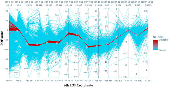
Figure 8.
Parallel coordinates of the MC-based 15 EOF scores obtained for the G2 generator.
5. Discussion and Conclusions
The problem of a lack of specific datasets for applying machine-learning-based DVAs has been tackled in this paper; a comprehensive methodology has been presented to perform MC-based simulations to test power systems to determine post-contingency dynamic data that can be used to train machine learning tools.
For this, a well-defined stochastic methodology that can be used to generate dynamic data has been presented, showing good performance. The proposed method is based on a Monte Carlo simulation whose comprehensive structure has been expanded upon in this paper. Further research is warranted to apply this method for the generation of dynamic data from the Ecuadorian national interconnected system for performing security assessments based on machine learning.
This methodology is applied as part of the project PVI-DEE-2023-01, “Dynamic security assessment of the national interconnected system using numerical and artificial intelligence methods”. Further research is under development for applying different machine learning tools to the data obtained from the proposed method to accomplish DVAs.
Funding
This research received no external funding.
Institutional Review Board Statement
Not applicable.
Informed Consent Statement
Not applicable.
Data Availability Statement
The data presented in this study are available on request from the corresponding author. The data are not publicly available due to intellectual property of universities.
Conflicts of Interest
The authors declare no conflict of interest.
Nomenclature
| AI | Artificial intelligence |
| DVA | Dynamic vulnerability assessment |
| EOF | Empirical orthogonal function |
| k | Weibull shape parameter |
| LLE | Largest Lyapunov exponent |
| MC | Monte Carlo |
| OPF | Optimal power flow |
| Probability distribution function | |
| PMU | Phasor measurement unit |
| SIME | Single machine equivalent |
| SIPS | System integrity protection scheme |
| SSS | Small signal stability |
| tcl | Fault clearing time |
| tr | Recovery time |
| tu | Unstable time |
| WAMS | Wide area monitoring system |
| η | Transient stability margin (η < 0: unstable, η > 0: stable) |
| λ | Weibull scale parameter |
| μ | Mean or expectation |
| σ | Standard deviation |
References
- Dong, Z.; Zhang, P. Emerging Techniques in Power System Analysis; Springer: Berlin/Heidelberg, Germany, 2010. [Google Scholar]
- Rueda, J.L. Evaluación y Mejora de la Estabilidad de Pequeña Señal de Sistemas Eléctricos de Potencia Considerando Incertidumbres. Ph.D. Thesis, Universidad Nacional de San Juan, San Juan, Argentina, 2009. [Google Scholar]
- Cepeda, J. Evaluación de la Vulnerabilidad del Sistema Eléctrico de Potencia en Tiempo Real usando Tecnología de Medición Sincrofasorial. Ph.D. Thesis, Universidad Nacional de San Juan, San Juan, Argentina, 2013. [Google Scholar]
- Rueda-Torres, J.L.; González-Longatt, F.; Cepeda, J. Dynamic Vulnerability Assessment and Intelligent Control: For Sustainable Power Systems; John Wiley & Sons: Hoboken, NJ, USA, 2018. [Google Scholar]
- Echeverria, D. Evaluación y Mejora de la Estabilidad Transitoria de Sistemas Eléctricos en Tiempo Real Utilizando PMUs. Ph.D. Thesis, Universidad Nacional de San Juan, San Juan, Argentina, 2021. [Google Scholar]
- Vaca, S. Evaluación Predictiva de Estabilidad Transitoria en Tiempo Real Mediante Aprendizaje Automático y la Identificación de Patrones del Máximo Exponente de Lyapunov. Master’s Thesis, Escuela Politecnica Nacional, Quito, Ecuador, 2023. [Google Scholar]
- Kumar, C.S.; Karuppiah, N.; Kumar, B.P.; Shitharth, S.; Dasu, B. Improvement of the Resilience of a Microgrid Using Fragility Modeling and Simulation. J. Electr. Comput. Eng. 2022, 3074298. [Google Scholar]
- Hashish, M.S.; Hasanien, H.M.; Ji, H.; Alkuhayli, A.; Alharbi, M.; Akmaral, T.; Turky, R.A.; Jurado, F.; Badr, A.O. Monte Carlo simulation and a clustering technique for solving the probabilistic optimal power flow problem for hybrid renewable energy systems. Sustainability 2023, 15, 783. [Google Scholar] [CrossRef]
- Alsharif, A.; Tan, C.W.; Ayop, R.; Al Smin, A.; Ahmed, A.A.; Kuwil, F.H.; Khaleel, M.M. Impact of electric Vehicle on residential power distribution considering energy management strategy and stochastic Monte Carlo algorithm. Energies 2023, 16, 1358. [Google Scholar] [CrossRef]
- Hinojosa, V.H. Pronóstico de Demanda de Corto Plazo en Sistemas de Suministro de Energía Eléctrica Utilizando Inteligencia Artificial. Ph.D. Thesis, Universidad Nacional de San Juan, San Juan, Argentina, 2007. [Google Scholar]
- Chen, C.L.; Chen, S.L. Short-term Unit Commitment with Simplified Economic Dispatch. Electr. Power Syst. Res. 1991, 21, 115–120. [Google Scholar] [CrossRef]
- Hedman, K.W.; Oren, S.S.; O’Neill, R.P. A review of transmission switching and network topology optimization. In Proceedings of the 2011 IEEE Power and Energy Society General Meeting, Detroit, MI, USA, 24–28 July 2011; pp. 1–7. [Google Scholar]
- Li, W. Risk Assessment of Power Systems: Models, Methods, and Applications; IEEE Press Series on Power Engineering; IEEE: Piscataway, NJ, USA, 2005. [Google Scholar]
- Cepeda, J.C.; Colomé, D.G. Benefits of empirical orthogonal functions in pattern recognition applied to vulnerability assessment. In Proceedings of the 2014 IEEE PES Transmission & Distribution Conference and Exposition—Latin America (PES T&D-LA), Medellin, Colombia, 10–13 September 2014; pp. 1–6. [Google Scholar]
- Rosenstein, M.; Collins, J.; Luca, C. A Practical Method for Calculating Largest Lyapunov Exponents from Small Data Sets; NeuroMuscular Research Center and Department of Biomedical Engineering: Boston, UK, 1992. [Google Scholar]
Disclaimer/Publisher’s Note: The statements, opinions and data contained in all publications are solely those of the individual author(s) and contributor(s) and not of MDPI and/or the editor(s). MDPI and/or the editor(s) disclaim responsibility for any injury to people or property resulting from any ideas, methods, instructions or products referred to in the content. |
© 2023 by the author. Licensee MDPI, Basel, Switzerland. This article is an open access article distributed under the terms and conditions of the Creative Commons Attribution (CC BY) license (https://creativecommons.org/licenses/by/4.0/).

