Proceeding Paper

Air Quality Monitoring in a Near-City Industrial Zone by Low-Cost Sensor Technologies: A Case Study †

ENEA-Italian National Agency for New Technologies, Energy and Sustainable Economic Development, Laboratory of Functional Materials and Technologies for Sustainable Applications, Brindisi Research Centre, Strada Statale 7, Appia, Km. 706, 72100 Brindisi, Italy
*
Author to whom correspondence should be addressed.
Presented at the 2nd International Electronic Conference on Chemical Sensors and Analytical Chemistry, 16–30 September 2023; Available online: https://csac2023.sciforum.net/.
Eng. Proc. 2023, 48(1), 26; https://doi.org/10.3390/CSAC2023-14910
Published: 26 September 2023

Abstract

:
Urban industrial areas are often a matter of concern due to the emission of air pollutants that may affect the air quality of adjacent cities. Aerosol pollutants are monitored by governmental agencies that employ regulatory monitoring stations which are very accurate, but also very expensive, bulky, and demanding in terms of maintenance. For this reason, it often happens that the monitoring of the air quality in large areas is covered by few stations. This situation can lead to the building of air pollutant maps with low spatio-temporal resolution. An appealing way to address this issue is represented by low-cost miniaturized gas sensors (LCSs) employed in low-cost air quality monitors (LCMs). Despite the various and unquestionable points of strength characterizing these devices, the scientific community has raised several warnings about the accuracy of their measurements and issued many caveats regarding their use. In this study, a new LCM model designed and implemented in our laboratories was used to measure the NO2 and PM concentrations in the industrial area of Brindisi (Italy). Data gathered by the LCM were compared with reference instrumentations for a rigorous analysis of the performance achievable through these low-cost technologies in this particular case.

1. Introduction

Several studies have demonstrated the existence of a direct link between exposure to air pollutants and issues concerning public health [1,2]. Air pollution levels are monitored via the equipment of governmental agencies. However, the use of this equipment is often characterized by high costs due to purchasing, maintenance, and logistical issues [3]. As a consequence, often times, few monitoring points are deployed in a territory, making it impossible to build air pollutant maps with an adequate spatio-temporal resolution [3,4]. This issue has been addressed in recent years by developing low-cost technologies, which have introduced the low-cost miniaturized sensors (LCSs) and the low-cost air quality monitors (LCMs) to the worldwide market [5,6]. The strong points of such devices are directly linked to their cheapness compared to the regulatory-grade equipment, their high portability grade, and their low power consumption [7]. The appealing characteristics of these technologies have also induced the scientific community to investigate their use in application areas very similar to the classic “air pollution monitoring”, such as in malodor detection near landfill sites [8,9]. However, the flip side of these technologies is represented by a lower accuracy of measurements compared to the regulatory-grade equipment due to the interfering effects of environmental variables, such as temperature and humidity, and also due to insufficient sensitivity and selectivity [3,10,11]. To improve the performance of LCSs and LCMs, various different strategies have been explored. The most promising of these appear to be the application of artificial neural networks (ANNs), multivariate linear regression (MLR) algorithms, or other machine learning techniques to the data representing the measurements performed through such devices [3,7,12,13,14,15,16,17,18].
In this work, an LCM called SentinAir was used to monitor the NO2, PM2.5 and PM10 concentrations in the industrial area of Brindisi (Italy). This site is located near the city center and, therefore, the concentrations of the aforementioned pollutants in this area can significantly affect the air quality in the adjacent locations. The LCM used in this experiment was equipped with several LCSs: these included several NO2B43F sensors provided by Alphasense [19] for NO2 detection, and three samples of PMS5003 sensors given by Plantower [20] for the purpose of measuring PM2.5 and PM10 concentrations.

2. Materials and Methods

The LCM used for this experiment is a device designed and implemented in the laboratory of the ENEA Research Center of Brindisi called SentinAir. A complete description of the hardware and the software of SentinAir can be found in articles published earlier [21,22]. The LCM was used to measure NO2, PM2,5, and PM10 concentrations in a location with coordinates of 40°38′03.6″ N, 17°58′39.0″ E. Device data quality was evaluated through the use of reference instruments. NO2 sensor measurements were compared using the 405nm NOx monitor by 2Btech [23], while the APM-2 by Comde-Derenda [24] was employed to assess PM measurements.
Regarding the performance indicators, the coefficient of determination (R2), the mean absolute error (MAE), and the root mean squared error (RMSE) were adopted to understand the grade of reliability of data provided by the LCSs. R2, MAE, and RMSE are defined as follows:
R 2   = i = 1 N s i s ¯ ( r i r ¯ ) 2 i = 1 N ( s i s ¯ ) 2 ( r i r ¯ ) 2
MAE = 1 N i = 1 N s i r i
RMSE = 1 N i = 1 N ( s i r i ) 2
where r i represents the i-th measurement of the reference, s i , is the i-th concentration value given by the sensor, N is the number of observations, s ¯ represents the average of the sensor concentration measurements, and r ¯ is the average of the reference measurements. Data elaboration was carried out using the Scikit-learn libraries written in Python language [25,26,27,28]. Python platform is an open source software freely downloadable from the purpose-built website [26].
The sampling rate of both LCM and reference instruments was set to 5 min, and therefore hourly averages were considered for each pollutant.
The analog output signals provided by the electrochemical sensors for NO2 measurements were converted into gas concentrations using a multi-layer perceptron (MLP) [29], which is an ANN already successfully used in previous works [14,30]. The MLP used in this work has three hidden layers composed of, respectively 150, 50, and 150 neurons; these ones have “logistic” activation functions (for further details, see [26,31]).
The PMS5003 sensors provide PM10 and PM2.5 concentrations as output; therefore, we compared their measurements with the reference ones and, subsequently, an MLR algorithm was applied to improve their performance. It is already known that ambient humidity is a source of error for optical PM sensors [32,33]. For this reason, the relative humidity and the raw PM concentrations given by the sensor outputs were selected as predictors for the MLR model [33].

3. Results

The NO2 measurements started on the 28 April 2023 and ended on the 2 May 2023 due to an unexpected breakdown of the reference instrument. The final dataset composed of hourly averages was split into two parts containing roughly the same number of records. The first one (the calibration period) was used to train the ANN, while the second one (the validation period) was used to validate the measurements. The predictors used as inputs for the ANN were the signals of the “working” and “auxiliary” electrodes of the NO2B43F sensors [19], as well as the relative humidity. In Table 1, some statistics of the environmental variables monitored are reported.
The performance indicators related to the two NO2 sensors installed inside the LCM are reported in Table 2.
In Figure 1, the plots of the time series referring to the NO2 measurements are shown to provide a better understanding of the LCS performance.
The PM measurements were carried out from the 22 May 2023 to the 4 July 2023. Due to an unexpected power failure, data from the 16 June to the 21 June were lost. The final dataset consisting of these hourly averages was split into two parts, each of them containing 1053 records: the first one was used for the “calibration” of the MLR model, while the second one for its “validation”.
In Table 3, some significant statistics about the most relevant environmental variables are summarized.
In Table 4, the performance indicators related to the raw measurements carried out using the LCM (without the application of the MLR algorithm) are reported; conversely, in Table 5, the performance indicators representing the improvements achieved through the application of the MLR algorithm are shown.
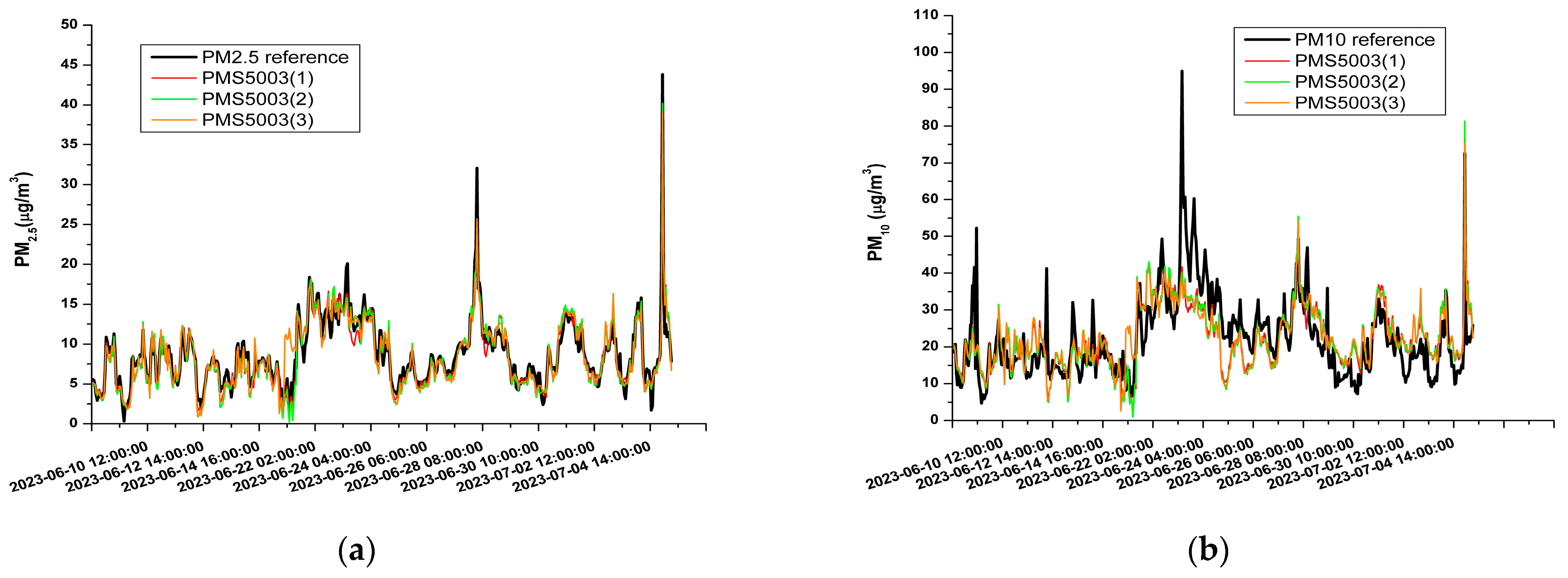
To offer a more intuitive view of the improvements achieved by considering the effect of the relative humidity, in Figure 2, the plots of the time series related to the PM sensor data after the application of the MLR algorithm are shown along with the reference measurements.

4. Discussion and Conclusions

The NO2 concentration levels were very low during the experiment (20.9 ppb as maximum value). By considering the validation period, this element has been determined to possess a poor capability to follow the trend of the reference for the NO2B43F(2) sensor (R2 = 0.005), and a moderate capability for the NO2B43F(1) (R2= 0.439). This difference is likely due to the different sensitivity characterizing the two sensors. As matter of fact, the sensor sensitivity can vary from 200 nA/ppm to 650 nA/ppm (see [19]). Namely, one sensor can have more than three times the sensitivity of another. This element can cause a remarkable difference in terms of R2. The global indication that we obtained from these data can be summarized by the fact that electrochemical sensors tested in this experiment have a limited capability to provide reliable measurements in cases of environments with very low levels of NO2 pollution.
The PM sensors under review demonstrated good performance in the case of PM2.5 measurements and moderate performance in the case of PM10 (see Table 4). By considering the relative humidity variable, we found that their performance was further improved. This aspect suggests to us that the measurements of PM2.5 provided by these sensors can be considered very reliable; conversely, in the case of PM10, we can conclude that their measurements are moderately reliable, despite considering the effect of relative humidity.

Author Contributions

Conceptualization, D.S.; methodology, D.S.; software, D.S.; validation, D.S.; formal analysis, D.S.; investigation, D.S.; resources, M.P. (Mario Prato); data curation, D.S.; writing-original draft preparation, D.S.; writing-review and editing, D.S.; visualization, D.S.; supervision, M.P. (Michele Penza); project administration, M.P. (Michele Penza); funding acquisition, M.P. (Michele Penza). All authors have read and agreed to the published version of the manuscript.

Funding

This research received no external funding.

Institutional Review Board Statement

Not applicable.

Informed Consent Statement

Not applicable.

Data Availability Statement

Please contact the author at [email protected].

Conflicts of Interest

The authors declare no conflict of interest.

References

  1. Kheirbek, I.; Wheeler, K.; Walters, S.; Kass, D.; Matte, T. PM2.5 and ozone health impacts and disparities in New York City: Sensitivity to spatial and temporal resolution. Air Qual. Atmos. Health 2013, 6, 473–486. [Google Scholar] [CrossRef] [PubMed]
  2. Makri, A.; Stilianakis, N.I. Vulnerability to air pollution health effects. Int. J. Hyg. Environ. Health 2018, 211, 326–336. [Google Scholar] [CrossRef]
  3. Karagulian, F.; Barbiere, M.; Kotsev, A.; Spinelle, L.; Gerboles, M.; Lagler, F.; Redon, N.; Crunaire, S.; Borowiak, A. Review of the Performance of Low-Cost Sensors for Air Quality Monitoring. Atmosphere 2019, 10, 506. [Google Scholar] [CrossRef]
  4. Suriano, D.; Cassano, G.; Penza, M. Design and Development of a Flexible, Plug-and-Play, Cost-Effective Tool for on-Field Evaluation of Gas Sensors. J. Sens. 2020, 2020, 8812025. [Google Scholar] [CrossRef]
  5. Kumar, P.; Morawska, L.; Martani, C.; Biskos, G.; Neophytou, M.; DiSabatino, S.; Bell, M.; Norford, L.; Britter, R. The rise of low-cost sensing for managing air pollution in cities. Environ. Int. 2015, 75, 199–205. [Google Scholar] [CrossRef]
  6. Snyder, E.G.; Watkins, T.H.; Solomon, P.A.; Thoma, E.D.; Williams, R.W.; Hagler, G.S.; Shelow, D.; Hindin, D.A.; Kilaru, V.J.; Preuss, P.W. The Changing Paradigm of Air Pollution Monitoring. Environ. Sci. Technol. 2013, 47, 11369–11377. [Google Scholar] [CrossRef]
  7. Suriano, D.; Penza, M. Assessment of the Performance of a Low-Cost Air Quality Monitor in an Indoor Environment through Different Calibration Models. Atmosphere 2022, 13, 567. [Google Scholar] [CrossRef]
  8. Suriano, D.; Rossi, R.; Alvisi, M.; Cassano, G.; Pfister, V.; Penza, M.; Trizio, L.; Brattoli, M.; Amodio, M.; De Gennaro, G.A. Portable Sensor System for Air Pollution Monitoring and Malodours Olfactometric Control. In Sensors and Microsystems: AISEM 2011 Proceedings; Lecture Notes in Electrical Engineering; Springer: Boston, MA, USA, 2012; Volume 109. [Google Scholar]
  9. Guidi, V.; Carotta, M.C.; Fabbri, B.; Gherardi, S.; Giberti, A.; Malagù, C. Array of sensors for detection of gaseous malodors in organic decomposition products. Sens. Actuators B Chem. 2012, 174, 349–354. [Google Scholar] [CrossRef]
  10. Lewis, A.; Edwards, P. Validate personal air-pollution sensors. Nature 2016, 535, 29–31. [Google Scholar] [CrossRef]
  11. Kang, Y.; Aye, L.; Ngo, T.D.; Zhou, J. Performance evaluation of low-cost air quality sensors: A review. Sci. Total Environ. 2022, 818, 151769. [Google Scholar] [CrossRef]
  12. Trizio, L.; Brattoli, M.; DeGennaro, G.; Suriano, D.; Rossi, R.; Alvisi, M.; Cassano, G.; Pfister, V.; Penza, M. Application of artificial neural networks to a gas sensor-array database for environmental monitoring. In Sensors and Microsystems; Springer: Boston, MA, USA, 2012; pp. 139–144. [Google Scholar]
  13. Bigi, A.; Mueller, M.; Grange, S.K.; Ghermandi, G.; Hueglin, C. Performance of NO, NO2 low cost sensors and three calibration approaches within a real world application. Atmos. Meas. Technol. 2018, 11, 3717–3735. [Google Scholar] [CrossRef]
  14. Spinelle, L.; Gerboles, M.; Villani, M.G.; Aleixandre, M.; Bonavitacola, F. Field calibration of a cluster of low-cost available sensors for air quality monitoring. Part A: Ozone and nitrogen dioxide. Sens. Actuators B Chem. 2015, 215, 249–257. [Google Scholar] [CrossRef]
  15. Yamamoto, K.; Togami, T.; Yamaguchi, N.; Ninomiya, S. Machine Learning-Based Calibration of Low-Cost Air TemperatureSensors Using Environmental Data. Sensors 2017, 17, 1290. [Google Scholar] [CrossRef] [PubMed]
  16. Si, M.; Xiong, Y.; Du, S.; Du, K. Evaluation and calibration of a low-cost particle sensor in ambient conditions using machine-learning methods. Atmos. Meas. Technol. 2020, 13, 1693–1707. [Google Scholar] [CrossRef]
  17. Cordero, J.M.; Borge, R.; Narros, A. Using statistical methods to carry out infield calibrations of low cost air quality sensors. Sens. Actuators B Chem. 2018, 267, 245–254. [Google Scholar] [CrossRef]
  18. Kosmopoulos, G.; Salamalikis, V.; Pandis, S.N.; Yannopoulos, P.; Bloutsos, A.A.; Kazantzidis, A. Low-cost sensors for measuring airborne particulate matter: Field evaluation and calibration at a South-Eastern European site. Sci. Total Environ. 2020, 748, 141396. [Google Scholar] [CrossRef]
  19. NO2-B43F Sensor Datasheet. Available online: https://www.alphasense.com/wp-content/uploads/2022/09/Alphasense_NO2-B43F_datasheet.pdf (accessed on 26 June 2023).
  20. PMS5003 Sensor Datasheet. Available online: https://www.plantower.com/en/products_33/74.html (accessed on 26 June 2023).
  21. Suriano, D. A portable air quality monitoring unit and a modular, flexible tool for on-field evaluation and calibration of low-cost gas sensors. HardwareX 2021, 9, e00198. [Google Scholar] [CrossRef] [PubMed]
  22. Suriano, D. SentinAir system software: A flexible tool for data acquisition from heterogeneous sensors and devices. SoftwareX 2020, 12, 100589. [Google Scholar] [CrossRef]
  23. Model 405nm Monitor. Available online: https://twobtech.com/model-405-nm-nox-monitor.html (accessed on 26 June 2023).
  24. APM-2 Monitor. Available online: https://www.comde-derenda.com/produkte/apm-2-2 (accessed on 26 June 2023).
  25. Python Website. Available online: https://www.python.org (accessed on 26 June 2023).
  26. Scikit Website. Available online: https://scikit-learn.org/stable/index.html (accessed on 26 June 2023).
  27. Buitinck, L.; Louppe, G.; Blondel, M.; Pedregosa, F.; Mueller, A.; Grisel, O.; Niculae, V.; Prettenhofer, P.; Gramfort, A.; Grobler, J.; et al. API design for machine learning software: Experiences from the scikit-learn project. arXiv 2013, arXiv:1309.0238. Available online: https://arxiv.org/abs/1309.0238v1 (accessed on 26 June 2023).
  28. Pedregosa, F.; Varoquaux, G.; Gramfort, A.; Michel, V.; Thirion, B.; Grisel, O.; Blondel, M.; Prettenhofer, P.; Weiss, R.; Dubourg, V.; et al. Scikit-learn: Machine Learningin Python. J. Mach. Learn. Res. 2011, 12, 2825–2830. [Google Scholar]
  29. Rumelhart, D.E.; McClelland, J.L.; PDP ResearchGroup (Eds.) Parallel Distributed Processing: Explorations in the Microstructure of Cognition; MIT Press: Cambridge, MA, USA, 1986. [Google Scholar]
  30. Spinelle, L.; Gerboles, M.; Villani, M.G.; Aleixandre, M.; Bonavitacola, F. Field calibration of a cluster of low-cost commercially available sensors for air quality monitoring. Part B: NO, CO and CO2. Sens. Actuators B Chem. 2017, 238, 706–715. [Google Scholar] [CrossRef]
  31. Bishop, C.M. Neural Networks for Pattern Recognition; Oxford University Press Inc.: New York, NY, USA, 1995. [Google Scholar]
  32. Suriano, D.; Prato, M. An Investigation on the Possible Application Areas of Low-Cost PM Sensors for Air Quality Monitoring. Sensors 2023, 23, 3976. [Google Scholar] [CrossRef] [PubMed]
  33. Lee, H.; Kang, J.; Kim, S.; Im, Y.; Yoo, S.; Lee, D. Long Term Evaluation and Calibration of Low-Cost Particulate Matter (PM) Sensor. Sensors 2020, 20, 3617. [Google Scholar] [CrossRef] [PubMed]
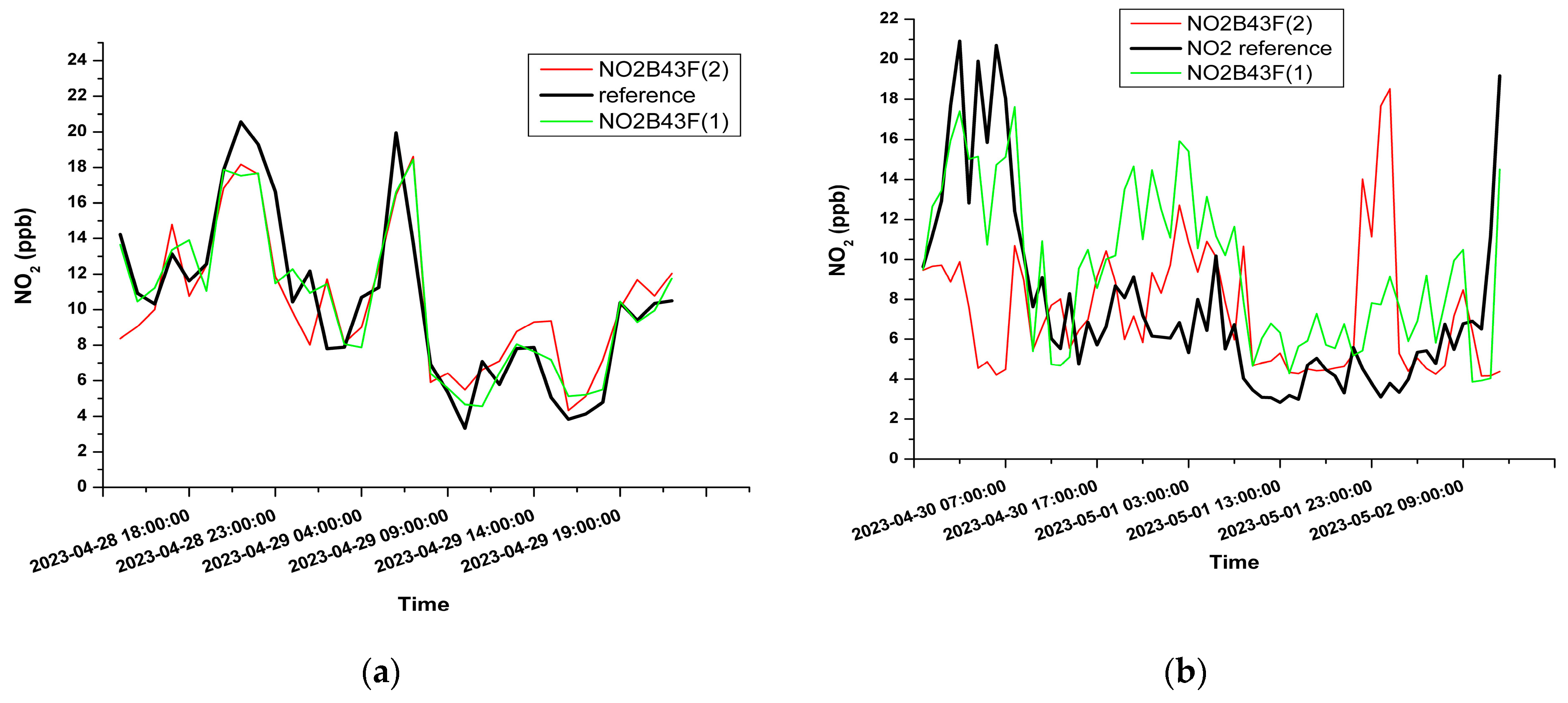
Figure 1. Time series of NO2 measurements related to: (a) the calibration or training period of the ANN; (b) the validation of the ANN predictions.
Engproc 48 00026 g001
Figure 2. Time series plots of the PM data in the validation period related to: (a) PM2.5 measurements; (b) PM10 measurements.
Engproc 48 00026 g002
Table 1. Statistics of the environmental variables monitored during the NO2 measurements.
Calibration PeriodValidation Period
MinMaxMedianMinMaxMedian
NO2 [ppb]3.320.610.42.820.96.3
T [°C]122620132617
RH[%]327849438873
Table 2. Performance indicators of NO2 sensors.
Calibration PeriodValidation Period
R2MAE [ppb]RMSE [ppb]R2MAE [ppb]RMSE [ppb]
NO2B43F(1)0.8181.42.00.4393.43.6
NO2B43F(2)0.7271.92.40.0053.85.9
Table 3. Statistics of the environmental variables monitored during the PM measurements.
Calibration PeriodValidation Period
MinMaxMedianMinMaxMedian
PM2.5 [µg/m3]4.229.310.00.343.88.0
PM10 [µg/m3]10.254.824.84.694.920
T [°C]173424203826
RH[%]288062268859
Table 4. Data related to the three sensors installed in the LCM under test and to the dataset composed of raw measurements.
R2MAE [µg/m3]RMSE [µg/m3]
PMS5003(1)PM100.4117.99.6
PMS5003(2)0.3917.510.0
PMS5003(3)0.3598.310.8
PMS5003(1)PM2.50.8599.911.3
PMS5003(2)0.85412.514.0
PMS5003(3)0.83514.215.8
Table 5. Data related to the three sensors installed in the LCM under test. The performance indicators were computed for both the calibration and the validation dataset.
Calibration PeriodValidation Period
R2MAE [µg/m3]RMSE [µg/m3]R2MAE [µg/m3]RMSE [µg/m3]
PMS5003(1)PM100.5674.96.80.4955.87.8
PMS5003(2)0.5415.16.90.4815.97.9
PMS5003(3)0.5335.27.00.4486.18.1
PMS5003(1)PM2.50.8431.21.70.9060.91.3
PMS5003(2)0.8341.21.70.9071.01.3
PMS5003(3)0.8631.01.50.8631.01.5
Disclaimer/Publisher’s Note: The statements, opinions and data contained in all publications are solely those of the individual author(s) and contributor(s) and not of MDPI and/or the editor(s). MDPI and/or the editor(s) disclaim responsibility for any injury to people or property resulting from any ideas, methods, instructions or products referred to in the content.