Proceeding Paper

Analyzing Seasonality in Hydropower Plants Energy Production and External Variables †

1
Faculty of Natural Science, University of Tirana, 1001 Tirana, Albania
2
Albanian Power Corporation, 1001 Tirana, Albania
*
Author to whom correspondence should be addressed.
Presented at the 7th International Conference on Time Series and Forecasting, Gran Canaria, Spain, 19–21 July 2021.
Eng. Proc. 2021, 5(1), 15; https://doi.org/10.3390/engproc2021005015
Published: 25 June 2021
(This article belongs to the Proceedings of The 7th International Conference on Time Series and Forecasting)

Abstract

:
This study is focused on energy production in Albania which involves different types of infrastructure at the various points of the energy production and distribution chain, as well as monitoring and early warning systems. At a time of rapid climate change, estimating the appropriate dimensions and design of such infrastructure and systems becomes crucial. The main objective is to analyze the seasonality pattern and main external climacteric factors, such as precipitation, average temperature, and water inflow. This work deals with the seasonality patterns of climacteric factors affecting energy production and considers different statistical learning methods for prediction.

1. Introduction

About 20% of the total installed capacity for electricity generation in Europe is from hydropower [1]. In Albania, the country’s needs for electricity are met mainly by the hydropower plants and less by the thermo power plants. The hydropower plants provide about 94% of the produced electricity, while the rest is produced by thermo power plants that use residual fuel oil as fuel and, in special cases, steam coal. Substantial drought in recent years has significantly reduced water levels for energy production in the Drin River cascade, generating by this way the lowest levels for the last 30 years. The cascade built in the Drin River basin is the largest not only for Albania but also in the Balkans for its installed capacity and the size of hydro technical works. The Albanian Electric Power Corporation (KESH), having in operation 79% of the production capacity in the country from the Drin cascade, manages to supply about 70–75% of the demand for electricity. KESH is not only one of the producers of electricity from important hydropower sources in the region, but it is also considered a factor with regional impact on the safety of hydro cycles [2].
Albania has established ALPEX as its energy exchange and electricity market operator which marks a further step towards the country’s integration as part of the European energy market and contributes to improving the investment climate in the country and attracting foreign investment in the energy sector [3,4]. The Albanian Energy Corporation (KESH) is the main public producer of electricity in the country and Drin is the longest river in the Albanian territories, with a length of 160 km. Figure 1 and Figure 2 show the position of the three HPP situated in Drin river cascade.
The approximate distance between the three HPPs is the same. Therefore, it is very important to take into account the fact that water flows through the Drin River and external sources (snowmelt, precipitation, etc.) are exploited through the cascade for energy production. Fierza, being the first HPP, uses natural inputs to produce energy and serves as a flow regulator for two ongoing HPPs. The electricity system in Albania is divided into three main sectors: the generation, transmission, and distribution sector. In Albania, the manufacture sector (KESH) produces energy based on the demands of the distribution operator (OSHE). So, why is it important to forecast power generation from HPPs in Albania? From this [5] 2018 report, Albania has a great potential for “hydroelectric energy” with eight main rivers crossing a river basin with over 57% of the current management extent, with an average altitude of 700 m above the level of sea and a perennial flow of 1245 m3/s, for a combined water supply of 40 billion cubic meters. An overview of the situation: 2100 MW the total installed capacity; Up to 615 MW of further potential capacity; above 1785 MW concession warded, eligible for partnerships. The water reserves valuing per capita second in the whole Europe makes the country offer an average cost of hydro production starting around 35 Euro/MWh.

2. Objective of the Study

Electricity demand and supply depend on many factors, the most important of which are climacteric indicators. In the production of electricity through hydropower plants, water resources play an important role. Among the factors that are likely to affect both variability in the supply and absolute availability of water are decreasing snow cover, increases in rainfall in hilly areas, drier conditions in the lowlands, as well as reduction in the capacity of soils to retain water due to land degradation and impacts of multiple stressors on vegetation and forests. Soil saturation can lead to sudden peaks in water inflow, even with mild precipitation. Global weather systems are also destabilized, leading to longer consecutive periods of precipitation or dry weather, as well as changes in how overall dynamics play out at very local levels due to factors such as topography [6,7]. Thus, increased weather variability will mean that reducing risk becomes more important than optimizing infrastructure for typical conditions. Increasing energy production by using half-empty reservoirs it may not be a problem if this can reduce potential disasters. Although increased investment costs are mostly the result of measures to decrease vulnerability to future climate shifts, this may affect infrastructure and supply chains for other options as well, so that the cost of HPP relative to other energy sources with low Greenhouse Gases (GHG) emissions is not likely to change noticeably. However, other factors may change the relative cost and outcomes of investments, such as absolute reduction in water availability for a region, increasing opportunities for wind power, considering that weather systems will contain more energy, and reduced cost of solar technologies, as a result of large investments in improved technologies globally [8].The increased anticipated incidence of extreme events is an argument for choosing numerous small-scale power plants, rather than investing in large-scale power plants, to reduce the impacts of disasters. Smaller plants are easier to retrofit and adapt as climate conditions change over the coming years. Also, it becomes important to ensure energy supply and access with a wider mix and range of options, both to compensate for seasonal variability and reduced predictability, and to mitigate impacts of disasters.
One of the main objectives of this study is to analyze the seasonality pattern and the correlation among some climacteric external factors which may affect the energy production in the Drin cascade and further use these variables as explanatory variables in energy production. The prediction of the capacities of energy produced will help the stakeholders and decision makers (such as the government) to better take precautions on demand and supply of the energy for the country needs and region. Because Albania is heavily reliant on hydropower electricity production some vulnerability in the future may be the reduction of power generation due to severe drought which will result in less electricity produced by the hydropower plants. The heavy reliance on hydropower sources may be appropriate for reducing greenhouse gas emissions and improving air quality in Albania but can increase vulnerability to climate change. During last few years, a decrease in precipitation was observed and increased temperature in summer season as well. These changes could reduce annual average electricity output from Albania’s large hydropower plants (LHPPs) by about 15% and from small hydropower plants (SHPPs) by around 20% by 2050. Global climate change may affect the provision of energy from solar and wind generation. A likely increase in the global solar radiation and the hours of sunshine duration will lead to an increase in the use of solar energy for different energy services, but at the moment the main interest is focused on energy produced by HPP and the capacity of production. In their study, ref [9] point out that spring shifting to earlier in the season may leave reservoirs half-empty if managers expect later floods that never arrive, with adverse consequences for hydropower production and later winter floods is some coastal areas of the Mediterranean may encounter reservoirs that have already been filled which may increase downstream flood risk [9,10]. Also, unpredictable reservoir storage could affect hydroelectric power production and the energy market [11]. There are many research works focused on seasonality pattern of external factors affecting energy produced by HPP. A review of these works is presented in [12,13,14]. The relationship between energy production season and climacteric variables is also discussed in [15,16,17].

3. Time Series Analysis

Electricity produced by hydropower plants is likely to be influenced by climatic factors and their seasonal patterns. It is expected that underlying causal dynamics affecting water inflow will follow a seasonal pattern (related to snow smelting, precipitation, upstream water use, capacity of vegetation and soils to retain water), so that correlations to any single factor will vary over the year. The spatial distribution of precipitation, topography, and time-lag between the time of precipitation and time of water inflow need to be considered [18]. Crucially, for the future, domino effects are likely to arise connected to aspects such as the fact that existing water management systems, reservoirs, and natural bodies of water that retain water upstream will not be sufficient to handle extended periods of high precipitation or indeed, peaks connected to extreme weather. This leads to non-linear situations, and an asymmetry in the impacts of variability in terms of aspects of systems affected and the time scale. Wet periods (or rapid snow smelting) may also lead to short term flooding, infrastructure damage, and possibly dam collapse. Also, extended dry periods will lead to forest fires or collapse of forests due to drought and increase in diseases. Forests are also exposed to the increased force in wind, avalanches, landslides, and erosion in mountain areas connected to more intense precipitation. Impacts on forests have long term and sometimes irreversible consequences, which thus may affect future dynamics of hydropower energy production.
In this study, we have considered four time series with monthly observation and duration from January 1991 to December 2016, in total 312 observations. We considered the monthly average temperature (Celsius degree. Source World Bank); monthly average rainfall (in millimeters. Source: World Bank), Water inflow in Fierza (in m3/second, Source: KESH); and total energy produced by three HPP of Drin cascade (Fierza-Koman-VD measured in GWh, Source: KESH).
Previous studies were based on the analyses of these variables and their importance in energy production showing the effect of these variables in energy demand and production, and how seasonality patterns affect these components of energy sectoring Albania [19].
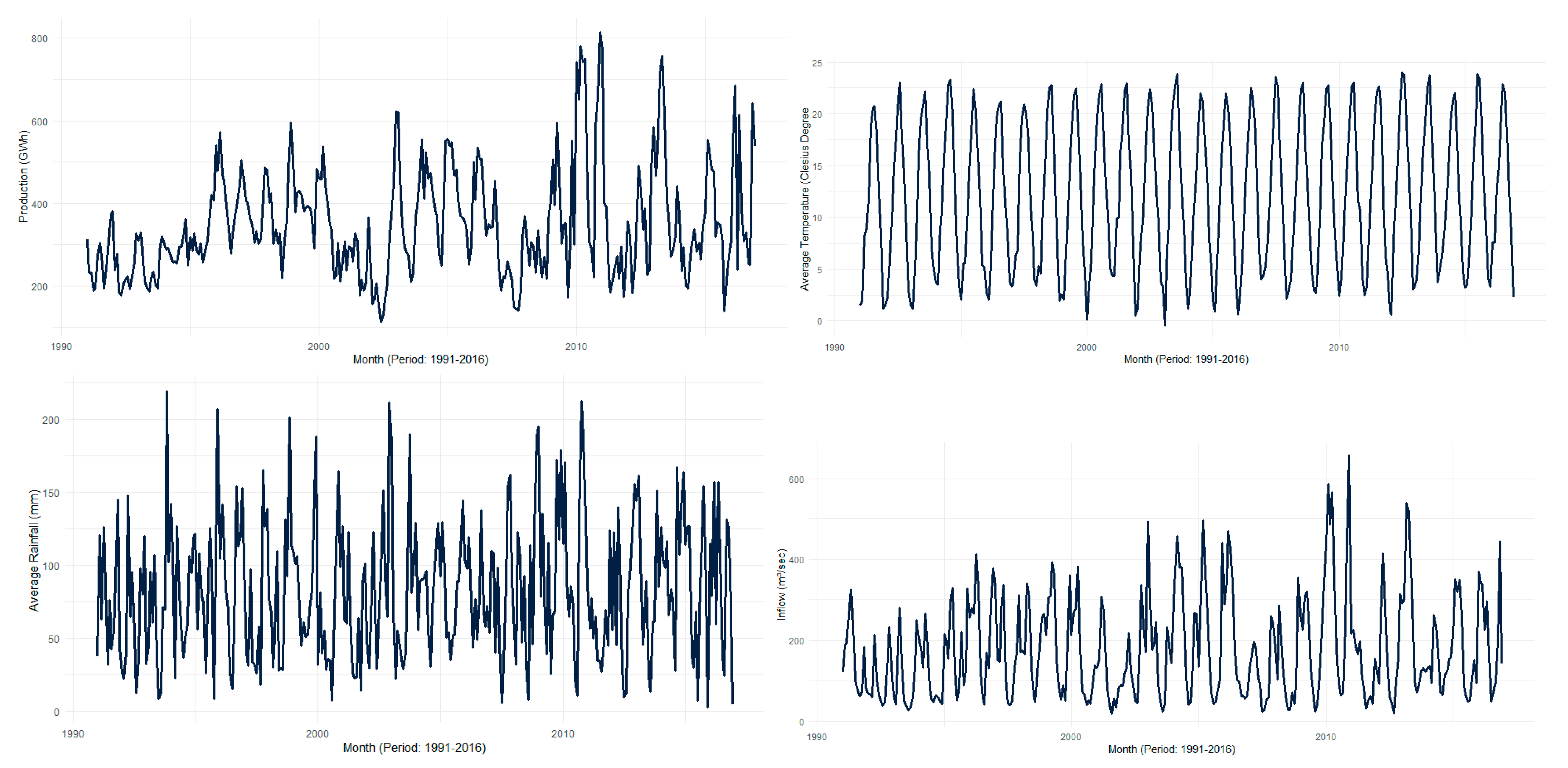
Observing the four time series in Figure 3, we can agree on the fact that no clear linear trend is observed and that perhaps a seasonal pattern is present in each of the time series. The time series have no missing data and the presence of outliers is not significant.
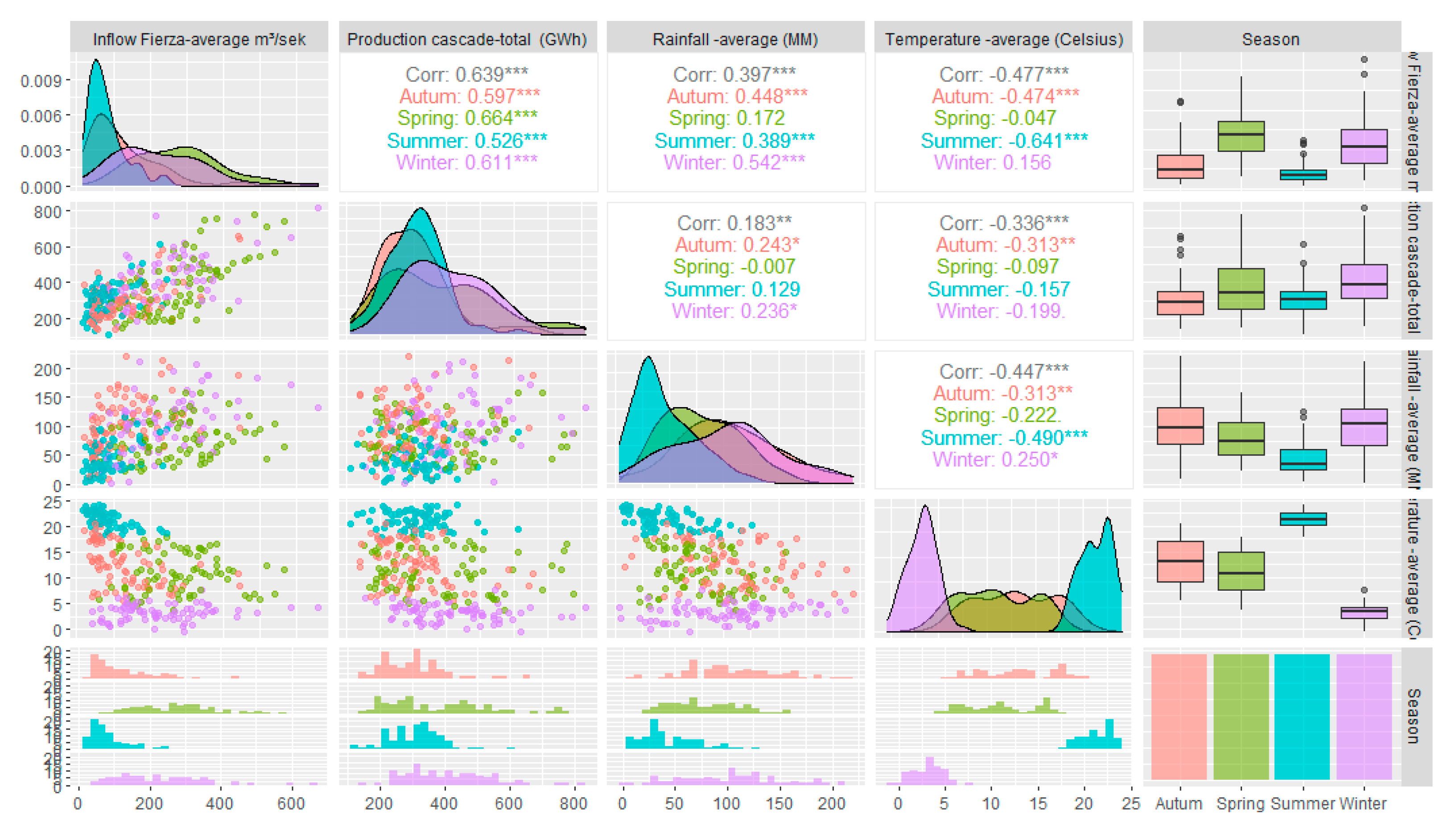
Figure 4 shows the correlation plot among the variables by season. We may notice that there is a clear positive correlation between inflows in Fierza and production of the cascade which is most evident and strong during spring season (correlation = 0.664) when precipitation and snowmelt flows are higher. Inflows in Fierza and rainfalls have a positive correlation during autumn and winter season (correlation = 0.542). For the water inflow time series and energy produced in the cascade (from three HPP), we observe a significant change during 2010. This change will be also analyzed in the seasonal plot below.
Given that Albania is a Mediterranean country where seasons are clearly observed, we expect seasonality in the pattern of the time series taken into consideration for the study. For a better view of the correlation among the time series chosen we can also use the correlation plot. The correlation plot shows a positive correlation between the energy produced and water inflow (correlation = 0.64). However, because of the fact that water inflow is not mainly affected by the precipitations we observe a low value of the correlation between production and rainfall. A negative correlation, also with a low value (correlation = −0.38) is observed between the production and the average temperature.
Given the monthly frequency of our data and the efficiency of such predictions in long term, we decided to use as training set 80% of the observations and as testing set 20% of the observations. Another issue was to take the observation for year 2010 in our train dataset. So, we decide to have this representation 80% (250 observations) and 20% (62 observations).
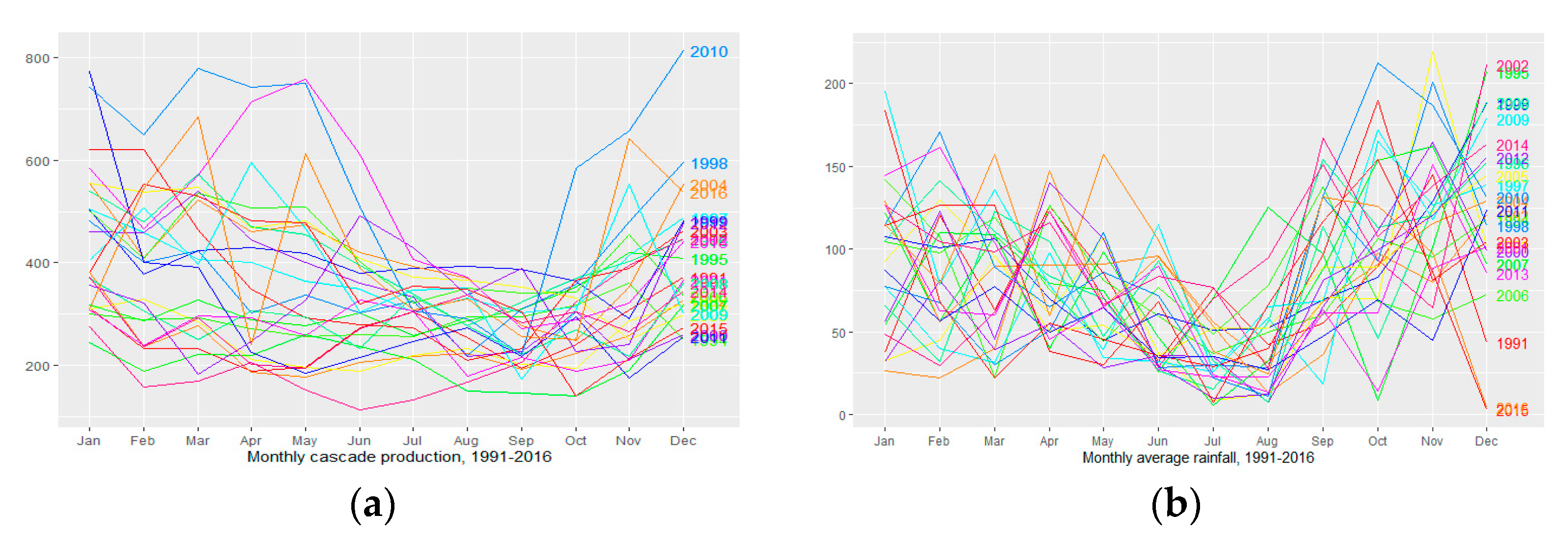
The seasonality of the monthly average temperature was confirmed by the seasonal graphs in Figure 5. The minimum average temperature is observed during winter and spring and the maximum average temperature is observed during the summer (July and August). The monthly average rainfall time series also expose presence of seasonality with high levels of rainfall during the wet months of autumn, winter and spring and with low levels during the summer. Carefully observing the seasonal plot for the time series of the water inflow, we can see the pattern of the time series for year 2010 which is significantly seen (in the two first seasonal plots) with high levels in almost all the months. We also observe high levels of inflows during the first months and the last months of the year. This phenomenon may be due to the increase in the level of inflows from natural causes such as precipitation and temperature which affects the snow melting and increase by this way the water level of the river Drin. We mention here again that the river cascade is positioned in the north side of Albania (the Alps). In the energy production time series, we also observe the same behavior as in the water inflow with high levels of production during the first months and the last months of the year. This is because the energy produced by HPP is positively correlated with the levels in the basin and water inflow.

4. Results

4.1. Models

The statistical time series models such as Naïve, autoregressive integrated moving average (ARIMA) [20] and exponential smoothing (Holt-Winters, ETS [21]) are most commonly used when it comes to monthly prediction especially with seasonality patterns. They have also become as popular as they are suitable for non-professionals, and they offer high accuracy and efficiency when it comes to non-complex time series data. Many competitions have shown that these methods outperform machine learning methods in many situations [22,23,24]. The advantage of classical univariate prediction methods is that they perform well when the volume of the data is considerable [25]. Neural networks are becoming more and more popular due to their ability to consider complexity and historical patterns in time series, being used as alternatives in different situations [26]. In this study our focus was to understand the relation between the external climacteric factors affecting the energy production by HPP. Below, we provide some results when using some statistical methods and neural networks with external variables which is the challenge for the future of our study.
We started by modeling our time series as a univariate time series and we also considered some statistical models using external factors among those presented above. Because the energy production time series show no linear trend, we decided not to go for the standard models such as naïve or drift because of the non-satisfactory visual results in prediction. ARIMA models consider in particular the linear behavior of the time series and stable seasonality; the ETS model takes into consideration the main components and in particularly the seasonality nature of the time series. Artificial Neural Networks (ANNs) are special mathematical models used also in prediction. They allow complex nonlinear relationships between the dependent variable and the independent(s) variable(s) used as explanatory variable(s). Neural networks are not based on an explicit stochastic model, so in most of the time we obtain prediction intervals by simulating future sample paths. The training process ofan ANN will depend on the activation function and the method used for finding the opportune weights recursively. Occasionally, we begin the training process of an ANN by choosing randomly the input values and then apply weights to each observation that will pass on information to a hidden layer where the information will be handled by an activation function. There are many studies on the performance of ANN in different types of data [27,28].
During the time series models progressions a considerable research is also made in the hybridization between ANN and classical time series models, in order to consolidate and benefit from the advantages of both models [29,30]. The automotive process is very easy in R, so we used forecast libraries which offer many facilities of these models [21,31].

4.2. Model Performance Measures

The accuracy of the models is evaluated based on accuracy measures such as error measures and information criteria. Bias and accuracy are then analyzed for every model and based on a critical judgment we have given our proposals for future work. The selection of the “best” model between all proposed was affected also on subjective indicators observed in the behavior of the time series such as seasonality [32,33]. Here, we used Mean Error (ME), Mean Absolute Error (MAE), Mean Absolute Percentage Error (MAPE), symmetric MAPE (sMAPE), and Root Mean Square Error (RMSE), calculated from the equations below:
M A E = 1 n i = 1 n | X ^ t X t |
M E = 1 n i = 1 n ( X ^ t X t )
M A P E = ( 1 n i = 1 n | X ^ t X t | | X t | ) 100 %
s M A P E = ( 1 n i = 1 n 2 | X ^ t X t | | X t | + | X ^ t | )
R M S E = 1 n i = 1 n ( X ^ t X t ) 2
where X t denote the observation at time t and X ^ t denote the estimated time series. Also, we graphed the fitted values (January 1991 up to January 2013) and the predicted values and compared them graphically with the testing time series (starting from February 2011 up to December 2016). For forecast of neural net models with external regressors, we need to have future values of the external regressor to be fed in the forecast function. We can use the test values for the inflow regressor. More than one external regressors can be used in the forecast procedure of neural network models. Error measurements should be small if the predicted values are close to the true values and will be large otherwise. The error measurements expressed in Figure 6 are computed using the training set used to fit the model and are referred to as the training errors. In general, we are focused on the accuracy of the predictions that we obtain when we apply a method to previously unseen test set, so we also calculate and evaluate the performance of the model based on out of sample set. From Figure 6, we observe that the Neural Network model (NNETAR) has the lowest values of the errors for the in-sample set compared to all the other models considered. We know that there is no guarantee that the method with the lowest training error will also have the lowest test error so we should evaluate the accuracy of the model based also in out-of-sample performance. Over fitting happens commonly when our statistical learning procedure is trying hard to discover patterns in the training set and we notice in most of the time low values for training set which are accompanied by large values for the testing set. Nonetheless, because many statistical learning methods seek to minimize the training error, we almost always expect these values to be smaller than the testing errors. Bias is also important when it comes to improving forecasting accuracy [34]. Bias is calculated as the average of the difference between the real values ( y i ) and the predicted values ( y ˜ i ) by the model: b i a s = m e a n ( y i y ˜ i ) .
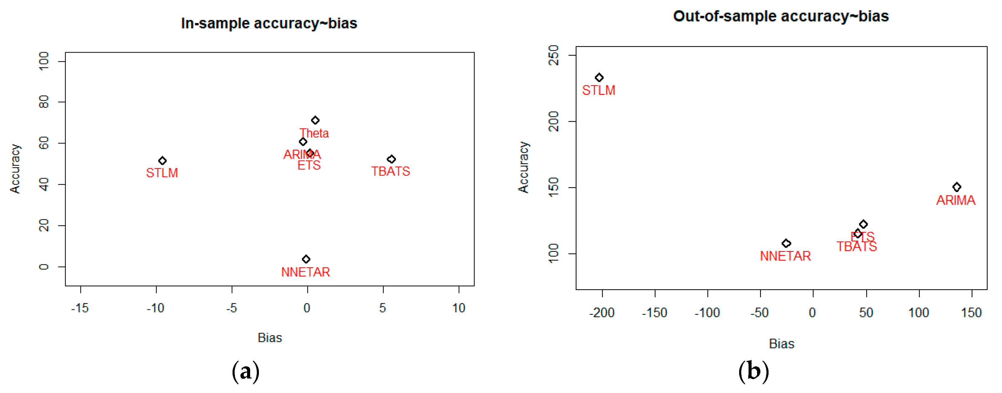
Figure 7 shows the situation of the in-sample and out-of-sample bias and accuracy (RMSE) for the proposed models. We notice that among the models, NN in both cases (in-sample and out-of-sample) has the lowest values of accuracy (RMSE) and bias (very close to 0). The fact that this model offers good performance indicators, in both sets, ranks it among the best models to be used for forecasting purposes. The artificial neural network learns using the patterns of the time series seasonal cycles.
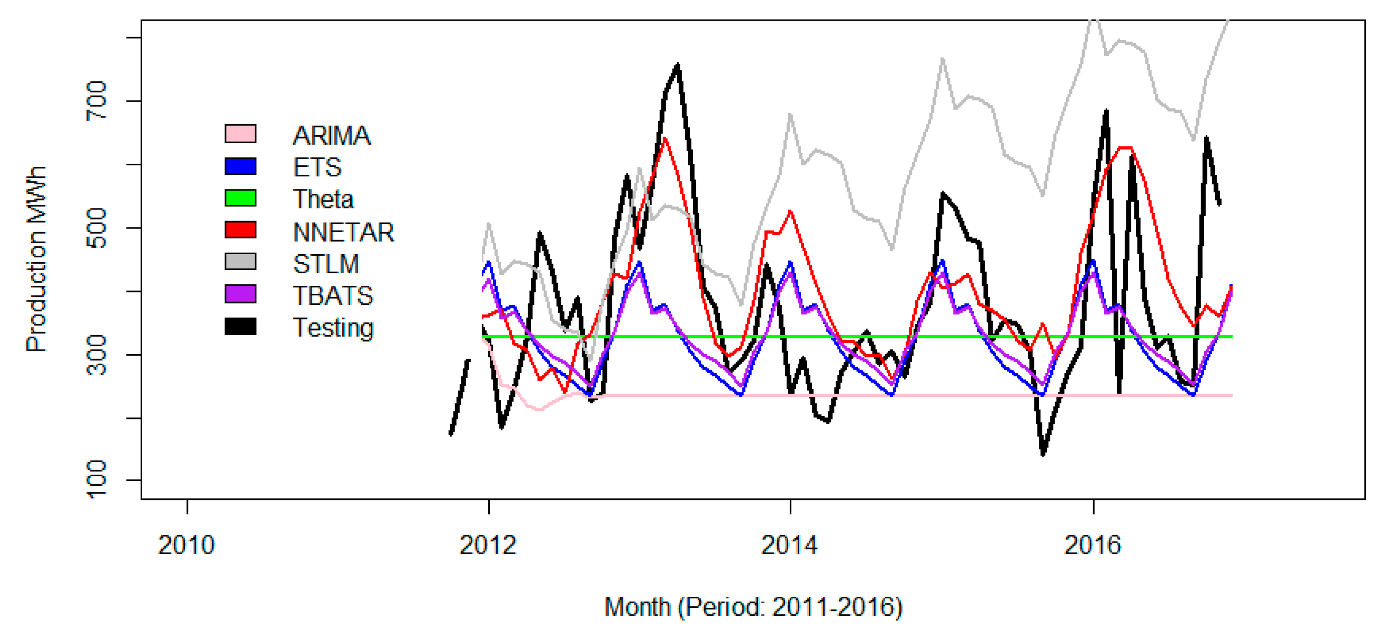
Figure 8 shows the comparison of accuracy versus bias of the proposed models for in-sample and out-of-sample data. We may observe that NNETAR has better accuracy and the lower bias for both in-sample and out-of-sample data compared to other models. Figure 9 shows the test data and forecasts according to each method reviewed in this study. Here, too, we graphically note the goodness of the NNETAR method in the prediction of monthly seasonal time series.

5. Conclusions

Electricity produced by hydropower plants is likely to be influenced by climatic factors and their seasonal patterns. As such, analyzing these patterns and the correlation among climacteric external factors is becoming one of the challenges to obtain accurate predictions of the amount of energy a hydropower plant could produce during a given season. Many statistical learning techniques are used to obtain accurate predictions such as ARIMA, ETS, NN, TBATS, STLM, etc. In this study, we analyzed the seasonality of patterns of the monthly average temperature, monthly average precipitations, monthly average inflow in the first HPP, and the total monthly amount of energy produced in the cascade of Drin River positioned in the Alps of Albania.
We are aware of the enormous work to be done with the data presented here, especially for the energy production by HPP which is highly affected by climacteric factors. We have considered many models which are chosen based on the seasonality cycles of the data. Among the models we tested, we observed and confirmed that neural networks have managed to capture these seasonal cycles and providing good forecasts for monthly energy produced in the cascade. At the end of this work, we must admit that there is always uncertainty that will affect our predictions and there is always a challenge to obtain better predictions through hybrid machine learning models.

Institutional Review Board Statement

Not applicable.

Informed Consent Statement

Not applicable.

Data Availability Statement

Not applicable.

References

  1. European Environment Agency (EEA). Report 2005. Available online: https://www.eea.europa.eu/publications/report_2005_0802_115659/at_download/file (accessed on 28 November 2020).
  2. KESH Albania. Available online: http://www.kesh.al/en/asset/drini-cascade/ (accessed on 28 November 2020).
  3. Available online: https://pressroom.ifc.org/all/pages/PressDetail.aspx?ID=26083 (accessed on 5 December 2020).
  4. Available online: https://crossbowproject.eu (accessed on 15 January 2021).
  5. Available online: https://adviser.albaniaenergy.org/wp-content/uploads/2018/11/Albania-hydroelectric-sector-towards-large-and-sustainable-developments-kept-by-Dr-Lorenc-Gordani.pdf (accessed on 15 January 2021).
  6. Martz, F.; Vuosku, J.; Ovaskainen, A.; Stark, S.; Rautio, P. The Snow Must Goon: Ground Ice Encasement, Snow Compaction and Absence of Snow Differently Cause Soil Hypoxia, CO2 Accumulation and Tree Seedling Damagein Boreal Forest. PLoS ONE 2016, 11, e0156620. [Google Scholar] [CrossRef]
  7. Confortola, G.; Soncini, A.; Bocchiola, D. Climate change will affect hydrological regimes in the Alps. J. Alp. Res. Rev. Géogr. Alp. 2013, 101–103. [Google Scholar] [CrossRef] [Green Version]
  8. Saberian, A.; Hizam, H.; Radzi, M.A.M.; AbKadir, M.Z.A.; Mirzaei, M. Modelling and Prediction of Photovoltaic Power Output Using Artificial Neural Networks. Int. J. Photoenergy 2014, 2014, 469701. [Google Scholar] [CrossRef] [Green Version]
  9. Blöschl, G.; Hall, J.; Parajka, J.; Perdigão, R.A.; Merz, B.; Arheimer, B.; Aronica, G.T.; Bilibashi, A.; Bonacci, O.; Borga, M.; et al. Climate Change Shifts the Timing of European Floods. Sci. News Science 2017, 357, 588–590. [Google Scholar] [CrossRef] [Green Version]
  10. Blöschl, G.; Hall, J.; Viglione, A.; Perdigão, R.A.; Parajka, J.; Merz, B.; Lun, D.; Arheimer, B.; Aronica, G.T.; Bilibashi, A.; et al. Changing climate both increases and decreases European river floods. Nature 2019, 573, 108–111. [Google Scholar] [CrossRef]
  11. Wagner, T.; Themeßl, M.; Schüppel, A.; Gobiet, A.; Stigler, H.; Birk, S. Impacts of climate change on stream flow and hydropower generation in the Alpineregion. Env. Earth Sci. 2017, 76, 1–22. [Google Scholar] [CrossRef] [Green Version]
  12. Engeland, K.; Borga, M.; Creutin, J.D.; François, B.; Ramos, M.H.; Vidal, J.P. Space-time variability of climate variables and intermittent renewable electricity production—A review. Renew. Sustain. Energy Rev. 2017, 79, 600–617. [Google Scholar] [CrossRef]
  13. Schaeffer, R.; Szklo, A.S.; de Lucena, A.F.; Borba, B.S.; Nogueira, L.P.; Fleming, F.P.; Troccoli, A.; Harrison, M.; Boulahya, M.S. Energy sector vulnerability to climate change: A review. Energy 2012, 38, 1–12. [Google Scholar] [CrossRef]
  14. Chandramowli, S.N.; Felder, F.A. Impact of climate change on electricity systems and markets—A review of models and forecasts. Sustain. Energy Technol. Assess 2014, 5, 62–74. [Google Scholar] [CrossRef]
  15. Sun, T.; Zhang, T.; Teng, Y.; Chen, Z.; Fang, J. Monthly Electricity Consumption Forecasting Method Based on X12 and STL Decomposition Model in an Integrated Energy System. Math. Prob. Eng. 2019, 2019, 9012543. [Google Scholar] [CrossRef]
  16. Usha, T.; Balamurugan, S. Seasonal Based Electricity Demand Forecasting Using Time Series Analysis. Circuits Syst. 2016, 7, 3320–3328. [Google Scholar] [CrossRef] [Green Version]
  17. Kalimoldayev, M.; Drozdenko, A.; Koplyk, I.; Marinich, T.; Ab-dildayeva, A.; Zhukabayeva, T. Analysis of modern approaches for the prediction of electric energy consumption. Open Eng. 2020, 10, 350–361. [Google Scholar] [CrossRef]
  18. Crochet, P.; Jóhannesson, T.; Jónsson, T.; Sigurðsson, O.; Björnsson, H.; Pálsson, F.; Barstad, I. Estimating the Spatial Distribution of Precipitation in Iceland Usinga Linear Model of Orographic Precipitation. J. Hydrometeorol. 2007, 8, 1285–1306. [Google Scholar] [CrossRef]
  19. Gjika, E.; Ferrja, A.; Kamberi, A. A Study on the Efficiency of Hybrid Models in Forecasting Precipitations and Water Inflow Albania Case Study. Adv. Sci. Technol. Eng. Syst. J. 2019, 4, 302–310. [Google Scholar] [CrossRef] [Green Version]
  20. Box, G.E.; Hunter, W.H.; Hunter, S. Statistics for Experimenters; John Wiley and Sons: New York, NY, USA, 1978; Volume 664. [Google Scholar]
  21. Hyndman, R.; Koehler, A.B.; Ord, J.K.; Snyder, R.D. Forecasting with Exponential Smoothing: The State Space Approach; Springer Science & Business Media: Secaucus, NJ, USA, 2008. [Google Scholar]
  22. Makridakis, S.; Hibon, M. The M3-Competition: Results, conclusions and implications. Int. J. Forecast. 2000, 16, 451–476. [Google Scholar] [CrossRef]
  23. Makridakis, S.; Spiliotis, E.; Assimakopoulos, V. The M4 competition: Results, findings, conclusion and way forward. Int. J. Forecast. 2018, 34, 802–808. [Google Scholar] [CrossRef]
  24. Makridakis, S.; Spiliotis, E.; Assimakopoulos, V. Statistical and machine learning forecasting methods: Concern and ways forward. PLoS ONE 2018, 13, e0194889. [Google Scholar] [CrossRef] [PubMed] [Green Version]
  25. Bandara, K.; Bergmeir, C.; Smyl, S. Forecasting across time series databases using recurrent neural networks on groups of similar series: A clustering approach. Expert Syst. Appl. 2020, 140, 112896. [Google Scholar] [CrossRef] [Green Version]
  26. Hewamalage, H.; Bergmeir, C.; Bandara, K. Recurrent Neural Networks for Time Series Forecasting: Current status and future directions. Int. J. Forecast. 2021, 37, 388–427. [Google Scholar] [CrossRef]
  27. Del Angel, R.G. Financial time series forecasting using Artificial Neural Networks. Rev. Mex. Econ. Finanz. Nueva Época 2020, 15, 105–122. [Google Scholar]
  28. Tealab, A. Time series forecasting using artificial neural networks methodologies: Asystematic review. Future Comput. Inform. J. 2018, 3, 334–340. [Google Scholar] [CrossRef]
  29. Wang, L.; Zou, H.; Su, J.; Li, L.; Chaudhry, S. An ARIMA-ANN hybrid model for time series forecasting. Syst. Res. Behav. Sci. 2014, 30, 244–259. [Google Scholar] [CrossRef]
  30. Young, C.C.; Liu, W.C.; Hsieh, W.L. Predicting the water level fluctuation in an alpine lake using physically based, artificial neural network, and time series forecasting models. Math. Probl. Eng. 2015, 2015, 708204. [Google Scholar] [CrossRef] [Green Version]
  31. Hyndman, R.J.; Khandakar, Y. Automatic Time Series Forecasting: The Forecast Package for R. J. Stat. Softw. 2008, 27, 1–22. [Google Scholar] [CrossRef] [Green Version]
  32. Hyndman, R.J.; Koehler, A.B. Another look at measures of forecast accuracy. Int. J. Forecast. 2006, 22, 679–688. [Google Scholar] [CrossRef] [Green Version]
  33. Hyndman, R.J. Measuring Forecast Accuracy. 2014. Available online: https://pdfs.semanticscholar.org/af71/3d815a7caba8dff7248ecea05a5956b2a487.pdf (accessed on 28 November 2020).
  34. Spiliotis, E.; Petropoulos, F.; Assimakopoulos, V. Improving the forecasting performance of temporal hierarchies. PLoS ONE 2019, 14, e0223422. [Google Scholar] [CrossRef] [Green Version]
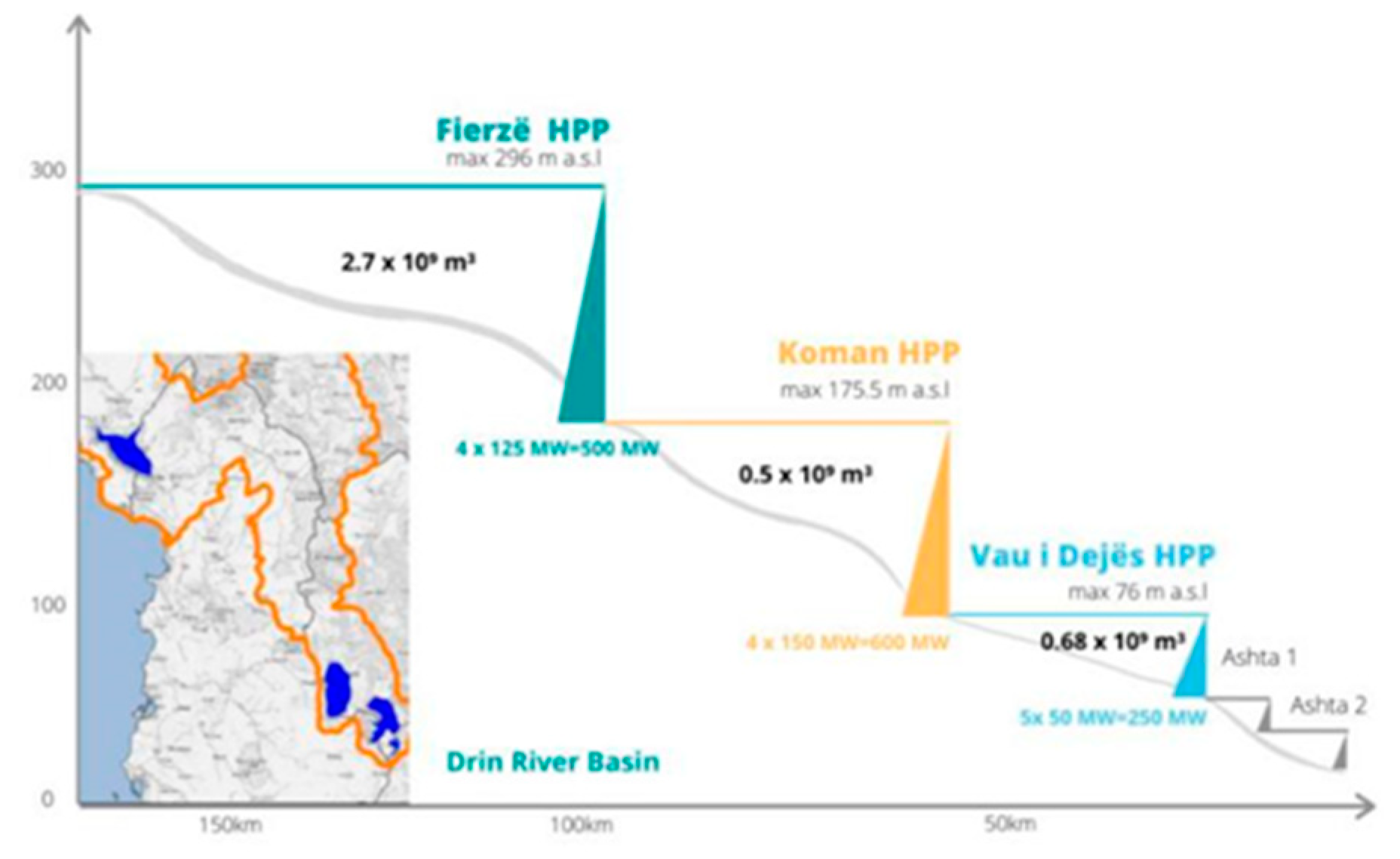
Figure 1. Drin cascade and the three main HPP (Source: http://www.kesh.al/en/asset/drini-cascade/ (accessed on 28 November 2020)).
Engproc 05 00015 g001
Figure 2. HPP in Drin cascade: Fierza, Koman and Vau-Dejes (Source: Google Earth).
Engproc 05 00015 g002
Figure 3. Time series of average temperature, average rainfall, water inflow, and energy produced by three HPP in Drin cascade.
Engproc 05 00015 g003
Figure 4. Correlation plot, Boxplot and density plot of the time series (Significance codes: * low correlation; ** average correlation; *** considerable correlation) (Source: Authors).
Engproc 05 00015 g004
Figure 5. Seasonal plot of the time series: (a) monthly total production; (b) monthly average rainfall) (period: 1991–2016) (Source: Authors).
Engproc 05 00015 g005
Figure 6. Seasonal plot of the time series: (a) monthly average temperature; (b) monthly average inflow) (period: 1991–2016) (Source: Authors).
Engproc 05 00015 g006
Figure 7. Error values for different models (in sample errors) (Source: Authors).
Engproc 05 00015 g007
Figure 8. (a) In-Sample; (b) Out-of-sample: accuracy versus bias of the proposed models.
Engproc 05 00015 g008
Figure 9. Predictions and testing data (Source: Authors).
Engproc 05 00015 g009
Publisher’s Note: MDPI stays neutral with regard to jurisdictional claims in published maps and institutional affiliations.