The Effect of Fear on a Diseased Prey–Predator Model with Predator Harvesting ^†

Abstract

In this paper, we examine the impact of fear in an eco-epidemiological model with predator harvesting and infection in a prey population. The effect of fear on susceptible prey due to infected prey was discussed. A predator consumes susceptible and infected prey at various rates in the form of a Holling type II Functional response. To examine the positivity and the boundedness of the solutions, the stability of all biologically feasible equilibrium points, and the Hopf bifurcation of the endemic equilibrium of the system, were derived. A numerical simulation was performed to support our analytical findings.

1. Introduction

Prey–predator models fall into two types: one is an ecological model and the other is an epidemiological model. The ecological model involves interactions between organisms, including humans, and their physical environment. Epidemiological models are used to study diseases in animals and humans. Also, the above study of ecology and epidemiology is called eco-epidemiology. In eco-epidemiology, we study prey–predator models with disease dynamics. Predator–prey interactions have been included in the Lotka–Volterra model for a very long time, see references [1,2,3]. In a similar vein, after the seminal work of Kermack and McKendrick [4], the interaction of the susceptible, infected, and recovered prey has been an interesting topic of study. The original predator–prey model was developed in large part by Vito Volterra and Alfred James Lotka. Ecology models and epidemiology models are the two basic categories into which mathematical models are often divided. In ecological models, the interactions between populations of a particular community are studied. Epidemiology models constitute the study of the spread of diseases between animals and humans. It is increasingly crucial to carry out research on the dynamics of illness within ecological systems. On the one hand, several studies of prey–predator dynamics have been conducted in recent decades, taking into account the impact of a range of biological characteristics, see, for example, reference [5]. Many mathematical models have been created and investigated in the field of epidemiology, taking into consideration various incidence rates and illnesses [6,7]. Ecology models and epidemiology models are the two basic categories into which mathematical models are often divided. There are three different forms of harvesting: constant, proportional to density, nonlinear, and others. All of these have been proposed and investigated [8]. There have been several suggestions for research harvesting methods, including harvesting continuously and depending on the density in proportional harvesting.

This piece is structured as follows: The prey–predator system’s past is described in Section 1. In Section 2, the mathematical formulation is presented. The existence of equilibrium points is described in Section 3. Local stability analyses are explained in Section 4. Hopf Bifurcation Analysis is found in Section 5. The results are presented numerically in Section 6. Finally, this paper concludes with a few observations about the suggested system in Section 7.

2. Model Formation

The system of the equation is as follows:

$$\begin{array}{c}\hfill \left.\begin{array}{cc}\frac{dX}{dT}=& \frac{r_{1}X}{1+fY}(1-\frac{X+Y}{K})-\lambda YX-\frac{{\alpha }_{1}XZ}{a_1+X},\\ \hfill \frac{dY}{dT}=& \lambda YX-d_{1}Y-\frac{b_{1}YZ}{a_1+Y},\\ \hfill \frac{dZ}{dT}=& -d_{2}Z+\frac{c{b}_{1}YZ}{a_1+Y}+\frac{c{\alpha }_{1}XZ}{a_1+X}-HEZ.\end{array}\right\}\end{array}$$

(1)

Then, the system changes to become non-dimensional. Here, $x=\frac{X}{K},y=\frac{Y}{K},z=\frac{Z}{K}$. Now, the system becomes

$$\begin{array}{c}\hfill \left.\begin{array}{cc}\frac{dx}{dt}=& \frac{rx(1-x-y)}{1+fy}-xy-\frac{\alpha xy}{a+x}\\ \frac{dy}{dt}=& yx-dy-\frac{\theta yz}{a+y}\\ \frac{dz}{dt}=& -\delta z+\frac{c\theta yz}{a+y}+\frac{c\alpha yz}{a+x}-hz\end{array}\right\}\end{array}$$

(2)

Here, the conditions are

$$\begin{array}{c}\hfill r=\frac{r_1}{\lambda K},\alpha =\frac{{\alpha }_1}{\lambda K},h=\frac{HE}{\lambda K},d=\frac{d_1}{\lambda K},\theta =\frac{b_1}{\lambda K},a=\frac{a_1}{K},\delta =\frac{d_2}{\lambda K},f=\frac{F}{K}\end{array}$$

Assuming the initial values are not negative $x\left(0\right)\ge 0,y\left(0\right)\ge 0,$ and $z\left(0\right)\ge 0$.

The detailed biological meanings of parameters are given in

Table 1. Biological meanings for the parameters.

Parameters	Biological Meaning
X	Susceptible Prey
Y	Infected Prey
Z	Predator
r	The intrinsic growth rate of prey
K	The carrying capacity of the environment
$a_1$	The half-saturation constant
${\alpha }_1$	Predation rate of susceptible prey
$b_1$	Predation rate of infected prey
c	Conversion coefficient from the prey to predator
$d_1$	The death rate of infected prey
$d_2$	The death rate of predator population
$\lambda$	The infection rate
H	The catchability coefficient of the predator
E	Harvesting effort

.

3. The Presence of Equilibrium Points

• The trivial equilibrium point $E_0(0,0,0)$.
• The diseased prey-free and predator-free equilibrium point $E_1(1,0,0)$.
• The predator-free equilibrium point $E_2(\overline{x},\overline{y},0)$,where
  $\overline{x}=d,\overline{y}=\frac{r(1-d)}{r+1}$.
• The infection-free equilibrium point $E_3(\overline{x},0,\overline{z})$, where
  $\overline{x}=\frac{a(\delta +h)}{c\alpha -\delta -h}$, and $\overline{z}=\frac{rac\left(\right(c\alpha -\delta -h)-a(\delta +h)}{{(c\alpha -\delta -h)}^2}$.
• The interior equilibrium point $E^{\ast }(x^{\ast },y^{\ast },z^{\ast })$,
  where $y^{\ast }=\frac{a(a(\delta +h)+((\delta +h)-c\alpha )s^{\ast })}{(c\alpha s^{\ast }+(c\theta -(\delta +h)(a+s^{\ast }))}$,
  $z^{\ast }=\frac{ac(s^{\ast }-d)(a+s^{\ast })}{(c\alpha s^{\ast }+(c\theta -(\delta +h)(a+s^{\ast }))}$,
  and $s^{\ast }$ is the unique positive root of the quadratic equation $A{S}^2+BS+C=0$,
  with $A=r(c\alpha +c\theta -(\delta +h\left)\right)$, $B=(c\theta -(\delta +h\left)\right)(-r+ar)-c\alpha r+a(\delta +h)+(\delta +h)-c\alpha \left)r\right)$, $C=-a\left(\right(r(c\theta -(\delta +h)+(c\alpha d-a(\delta +h)(1+r)\left)\right)$.

4. Analyses of Local Stability

Now, we want to calculate the Jacobian matrix for local stability analysis around different equilibrium points. The Jacobian matrix at an arbitrary point (x, y, z) is given by

$$J\left(E\right)=\left(\begin{array}{ccc}{w}_{11}& w_{12}& w_{13}\\ w_{21}& w_{22}& w_{23}\\ w_{31}& w_{32}& w_{33}\end{array}\right)$$

where,

$$\begin{array}{c}\hfill w_{11}=\frac{r(1-2x)}{1+fy}-y(\frac{r}{1+fy}+1)-\frac{\alpha az}{{(a+x)}^2},w_{12}=-x(\frac{r}{1+fy}+1),w_{21}=y\\ \hfill w_{13}=-\frac{rfx(1-x-y)}{{(1+fy)}^2}-\frac{\alpha x}{a+x},w_{22}=x-d-\frac{a\theta z}{{(a+y)}^2},w_{23}=\frac{-\theta y}{(a+y)},\\ \hfill w_{31}=\frac{ac\alpha z}{{(a+x)}^2},w_{32}=\frac{ac\theta z}{{(a+y)}^2},w_{33}=-\delta +\frac{c\theta y}{a+y}+\frac{\alpha cx}{a+x}-h.\end{array}$$

Theorem 1. 

The trivial equilibrium point $E_0(0,0,0)$ is always unstable.

Proof. 

Now, the corresponding Jacobian matrix $J\left(E_0\right)$ at $E_0(0,0,0)$ is given by

$$J\left(E_0\right)=\left(\begin{array}{ccc}r& 0& 0\\ 0& -d& 0\\ 0& 0& -h-\delta \end{array}\right)$$

The corresponding eigenvalues are r, $-d$, $-\delta -h$. One of the eigenvalues is positive. So, the trivial equilibrium point is always unstable. □

Theorem 2. 

The diseased prey-free and predator-free equilibrium point $E_1(1,0,0)$ is unstable.

Proof. 

The corresponding Jacobian matrix $J\left(E_1\right)$ at $E_1(1,0,0)$ is given by

$$J\left(E_1\right)=\left(\begin{array}{ccc}-r& -(r+1)& \frac{-\alpha }{a+1}\\ 0& -d+1& 0\\ 0& 0& -(\delta +h)+\frac{c\alpha }{a+1}\end{array}\right)$$

The corresponding eigenvalues are ${\lambda }_1=-r$, ${\lambda }_2=-d+1$, and ${\lambda }_3=-(\delta +h)+\frac{c\alpha }{a+1}$. Hence, $E_1(1,0,0)$ is unstable due to the numerical simulations. □

Theorem 3. 

The predator-free equilibrium point $E_2(\overline{x},\overline{y},0)$ is locally asymptotically stable if $(\delta +h)>\frac{c\alpha \overline{s}}{a+\overline{s}}+\frac{c\theta \overline{i}}{a+i}$.

Proof. 

The corresponding Jacobian matrix $J\left(E_2\right)$ at $E_2(\overline{x},\overline{y},0)$ is given by

$$J\left(E_2\right)=\left(\begin{array}{ccc}{f}_{11}& f_{12}& f_{13}\\ f_{21}& f_{22}& f_{23}\\ f_{31}& f_{32}& f_{33}\end{array}\right)$$

where,

$$\begin{array}{c}\hfill f_{11}=-rd,f_{12}=(-1-r)\widehat{x},f_{13}=-rfx(1-x-y)-\frac{\alpha \widehat{x}}{a+x},\\ \hfill f_{21}=y,f_{22}=0,f_{23}=\frac{-\theta \widehat{y}}{a+\widehat{y}},f_{31}=0,f_{32}=0,f_{33}=\frac{c\alpha \widehat{x}}{a+\widehat{x}}-\delta +\frac{c\theta \widehat{y}}{a+y}-h.\end{array}$$

The cubic characteristic equation of $J\left(E_2\right)$ is ${\lambda }^3+L{\lambda }^2+M\lambda +N=0$, where, $L=-f_{11}-f_{33},M=-f_{21}{f}_{12}+f_{33}{f}_{11},N=f_{12}{f}_{21}{f}_{33}$. If $L>0,N>0$, and $LM-N>0$, According to the criterion of Routh–Hurwitz, the negative real parts are the root of the above characteristic equation if and only if $L,N$ and $LM-N$ are positive. Hence, the $E_2$ is locally asymptotically stable. □

Theorem 4. 

The infection-free equilibrium point $E_3(\overline{s},0,\overline{p})$ is locally asymptotically stable if $\frac{a(\delta +h)}{c\alpha -\delta -h}-\frac{\theta \overline{p}}{a}<d$

Proof. 

$$J\left(E_3\right)=\left(\begin{array}{ccc}{a}_{11}& a_{12}& a_{13}\\ a_{21}& a_{22}& a_{23}\\ a_{31}& a_{32}& a_{33}\end{array}\right)$$

$$\begin{array}{cc}\hfill a_{11}& =r-\frac{2ar(\delta +h)}{c\alpha -\delta -h}-\frac{{(c\alpha -\delta -h)}^2\overline{p}}{a\alpha c^2},a_{12}=-\frac{a(1+r)(\delta +h)}{c\alpha -\delta -h},\hfill \\ \hfill a_{13}& =-\frac{(\delta +h)}{c},a_{21}=0,a_{22}=-d+\frac{a(\delta +h)}{c\alpha -\delta -h}-\frac{\theta \overline{p}}{a},\hfill \\ \hfill a_{31}& =\frac{{(c\alpha -\delta -h)}^2\overline{p}}{ac\alpha },a_{32}=\frac{c\theta \overline{p}}{a},a_{33}=0.\hfill \end{array}$$

The cubic characteristic equation of $J\left(E_3\right)$ is ${\lambda }^3+L{\lambda }^2+M\lambda +N=0$, where, $L=-a_{11}-a_{33},M=-a_{21}{a}_{12}+a_{33}{a}_{11},N=a_{12}{a}_{21}{a}_{33}$. If $L>0,N>0$, and $LM-N>0$, according to the criterion of Routh–Hurwitz, the negative real parts are the root of the above characteristic equation if and only if $L,N$ and $LM-N$ are positive. Hence, the $E_3$ is locally asymptotically stable. □

Theorem 5. 

The interior equilibrium point $E^{\ast }(x^{\ast },y^{\ast },z^{\ast })$ is locally asymptotically stable

if $L>0,N>0$, and $LM-N>0$

Proof. 

The corresponding Jacobian matrix at $E^{\ast }(s^{\ast },i^{\ast },p^{\ast })$ is given by

$J\left(E^{\ast }\right)=\begin{array}{c}\left(\begin{array}{ccc}{l}_{11}& l_{12}& l_{13}\\ l_{21}& l_{22}& l_{23}\\ l_{31}& l_{32}& l_{33}\end{array}\right)\end{array},$

where,

$$\begin{array}{c}\hfill l_{11}=-\frac{x\ast (-r+ar+(1+r)y^{\ast }+2r{x}^{\ast })}{a+x^{\ast }},l_{12}=-x^{\ast }(r+1),l_{13}=-\frac{\alpha x^{\ast }}{a+x^{\ast }},\\ \hfill l_{21}=y^{\ast },l_{22}=\frac{a\theta z^{\ast }{y}^2}{{(a+y^{\ast })}^2},l_{23}=-\frac{\theta y^{\ast }}{(a+y^{)}},l_{31}=\frac{ac\alpha z^{\ast }}{{(a+x^{\ast })}^2},l_{32}=\frac{ac\theta y^{\ast }}{{(a+x^{\ast })}^2},l_{33}=0.\end{array}$$

The cubic characteristic equation of $J\left(E^{\ast }\right)$ is ${\lambda }^3+L{\lambda }^2+M\lambda +N=0$. Here $L=-l_{11}-l_{33},M=-l_{21}{l}_{12}+l_{22}{l}_{11}-l_{13}{l}_{31}+l_{23}{l}_{32},N=l_{13}(-l_{22}{l}_{31}+l_{21}{l}_{32})+l_{23}(l_{12}{l}_{31}-l_{11}{l}_{32})$. If $L>0,N>0$, and $LM-N>0$. According to the criterion of Routh-Hurwitz, the negative real parts are the root of the above characteristic equation if and only if $L,N$ and $LM-N$ are positive. Hence, the interior equilibrium $E^{\ast }$ is locally asymptotically stable. □

5. Hopf Bifurcation Analysis

Theorem 6. 

If the critical value for the bifurcation parameter $q_1$ is exceeded, the model (2) experiences Hope-bifurcation. There exists the following Hopf bifurcation criteria at $q_1=q_1\ast 1.A_1(q_1\ast )A\left(q_1^{\ast }\right)-A_3\left(q_1^{\ast }\right)=0.$

Proof. 

For $h_1=q_1^{\ast }$,

$$\begin{array}{c}\hfill ({\lambda }^2\left(q_1^{\ast }\right)+A_2\left(q_1^{\ast }\right))(\lambda \left(q_1^{\ast }\right)+A_1\left(q_1^{\ast }\right))=0.\end{array}$$

(3)

⇒$\pm i\sqrt{A_2\left(q_1^{\ast }\right)}$ and $-A_1\left(q_1^{\ast }\right)$ be the zeros of the above equation. The following transversality requirement must be satisfied in order to achieve Hopf bifurcation at $q_1=q_1\ast$.

$$\frac{d}{d{q}_1^{\ast }}\left(Re\left(\lambda \left(q_1^{\ast }\right)\right)\right)|\ne 0.$$

The generic roots of the aforementioned equation are (3) for all $q_1$.

$$\begin{array}{c}\hfill {\lambda }_1=r\left(q_1\right)+is\left(q_1\right),\\ \hfill {\lambda }_2=r\left(q_1\right)-is\left(q_1\right),\\ \hfill {\lambda }_3=-A_1\left(q_1\right).\end{array}$$

Now, we examine the situation. $\frac{d}{d{q}_1^{\ast }}\left(Re\left(\lambda \left(q_1^{\ast }\right)\right)\right)|\ne 0.$

Let ${\lambda }_1=r\left(q_1\right)+is\left(q_1\right)$ in the (3), we obtain

$$\mathcal{A}\left(q_1\right)+i\mathcal{B}\left(q_1\right)=0.$$

where,

$$\begin{array}{cc}\hfill \mathcal{A}\left(q_1\right)& =r^3\left(q_1\right)+r^2\left(q_1\right)A_1\left(q_1\right)-3r\left(q_1\right)s^2\left(q_1\right)-s^2\left(q_1\right)A_{1}V+A_2\left(q_1\right)r\left(q_1\right)+A_1\left(q_1\right)A_2\left(q_1\right),\hfill \\ \hfill \mathcal{B}\left(q_1\right)& =A_2\left(q_1\right)s\left(q_1\right)+2r\left(q_1\right)s\left(q_1\right)A_1\left(q_1\right)+3r^2\left(q_1\right)s\left(q_1\right)+s^3\left(q_1\right).\hfill \end{array}$$

$$\begin{array}{cc}\hfill \frac{d\mathcal{A}}{d{q}_1}& ={\varsigma }_1\left(q_1\right)r^{{}^{\prime }}\left(q_1\right)-{\varsigma }_2\left(q_1\right)s^{{}^{\prime }}\left(q_1\right)+{\varsigma }_3\left(q_1\right)=0,\hfill \end{array}$$

(4)

$$\begin{array}{cc}\hfill \frac{d\mathcal{B}}{d{q}_1}& ={\varsigma }_2\left(q_1\right)r^{{}^{\prime }}\left(q_1\right)+{\varsigma }_1\left(q_1\right)s^{{}^{\prime }}\left(q_1\right)+{\varsigma }_4\left(q_1\right)=0,\hfill \end{array}$$

(5)

where,

$$\begin{array}{cc}\hfill {\varsigma }_1& =3r^2\left(q_1\right)+2r\left(q_1\right)A_1\left(q_1\right)-3s^2\left(q_1\right)+A_2\left(q_1\right),\hfill \\ \hfill {\varsigma }_2& =6r\left(q_1\right)s\left(q_1\right)+2s\left(q_1\right)a_1\left(q_1\right),\hfill \\ \hfill {\varsigma }_3& =r^2\left(q_1\right)A_1^{{}^{\prime }}\left(q_1\right)+s^2\left(q_1\right)A_1^{{}^{\prime }}\left(q_1\right)+A_2^{{}^{\prime }}\left(q_1\right)r\left(q_1\right),\hfill \\ \hfill {\varsigma }_4& =A_2^{{}^{\prime }}\left(q_1\right)s\left(q_1\right)+2r\left(q_1\right)s\left(q_1\right)A_1^{{}^{\prime }}\left(q_1\right).\hfill \end{array}$$

By multiplying (4) by ${\varsigma }_1\left(q_1\right)$ and (5) by ${\varsigma }_2\left(q_1\right)$, respectively,

$$\begin{array}{c}\hfill r{\left(q_1\right)}^{{}^{\prime }}=-\frac{{\varsigma }_1\left(q_1\right){\varsigma }_3\left(q_1\right)+{\varsigma }_2\left(q_1\right){\varsigma }_4\left(q_1\right)}{{{\varsigma }_1}^2\left(q_1\right)+{{\varsigma }_2}^2\left(q_1\right)}.\end{array}$$

(6)

Substituting $r\left(q_1\right)=0$ and $s\left(q_1\right)=\sqrt{A_2\left(q_1\right)}$ at $q_1=q_1^{\ast }$ on ${\varsigma }_1\left(q_1\right),{\varsigma }_2\left(q_1\right),{\varsigma }_3\left(q_1\right),$ and ${\varsigma }_4\left(q_1\right)$, we obtain

$$\begin{array}{cc}\hfill {\varsigma }_1\left(q_1^{\ast }\right)=& -2A_2\left(q_2^{\ast }\right),\hfill \\ \hfill {\varsigma }_2\left(q_1^{\ast }\right)=& 2A_1\left(q_1^{\ast }\right)\sqrt{A_2\left(q_1^{\ast }\right)}\hfill \\ \hfill {\varsigma }_3\left(q_1^{\ast }\right)=& A_3^{{}^{\prime }}\left(q_1^{\ast }\right)-A_2\left(q_1^{\ast }\right)A_1^{{}^{\prime }}\left(q_1^{\ast }\right),\hfill \\ \hfill {\varsigma }_4\left(q_1^{\ast }\right)=& A_2^{{}^{\prime }}\left(q_1^{\ast }\right)\sqrt{A_2{q}_1^{\ast }}.\hfill \end{array}$$

Equation (6), implies

$$\begin{array}{c}\hfill r^{{}^{\prime }}\left(q_1^{\ast }\right)=\frac{A_3^{{}^{\prime }}\left(q_1^{\ast }\right)-\left(A_1\left(q_1^{\ast }{A}_2\left(q_1^{\ast }\right)\right)\right)}{2(A_2\left(q_1^{\ast }\right)+A_1^2\left(q_1^{\ast }\right))},\end{array}$$

(7)

if $A_3^{{}^{\prime }}\left(q_1^{\ast }\right)-{\left(A_1\left(q_1^{\ast }\right)A_2\left(q_1^{\ast }\right)\right)}^{{}^{\prime }}\ne 0$⇒ $\frac{d}{d{q}_1^{\ast }}\left(Re\left(\lambda \left(q_1^{\ast }\right)\right)\right)|\ne 0,$ and ${\lambda }_3\left(q_1^{\ast }\right)=-A_1\left(q_1^{\ast }\right)\ne 0.$ $A_3^{{}^{\prime }}\left(q_1^{\ast }\right)-{\left(A_1\left(q_1^{\ast }\right)A_2\left(q_1^{\ast }\right)\right)}^{{}^{\prime }}\ne 0$ is ensured if the transversality criterion holds, and, at this point, the model (2) enters the Hopf bifurcation at $q_1=q_1^{\ast }$. □

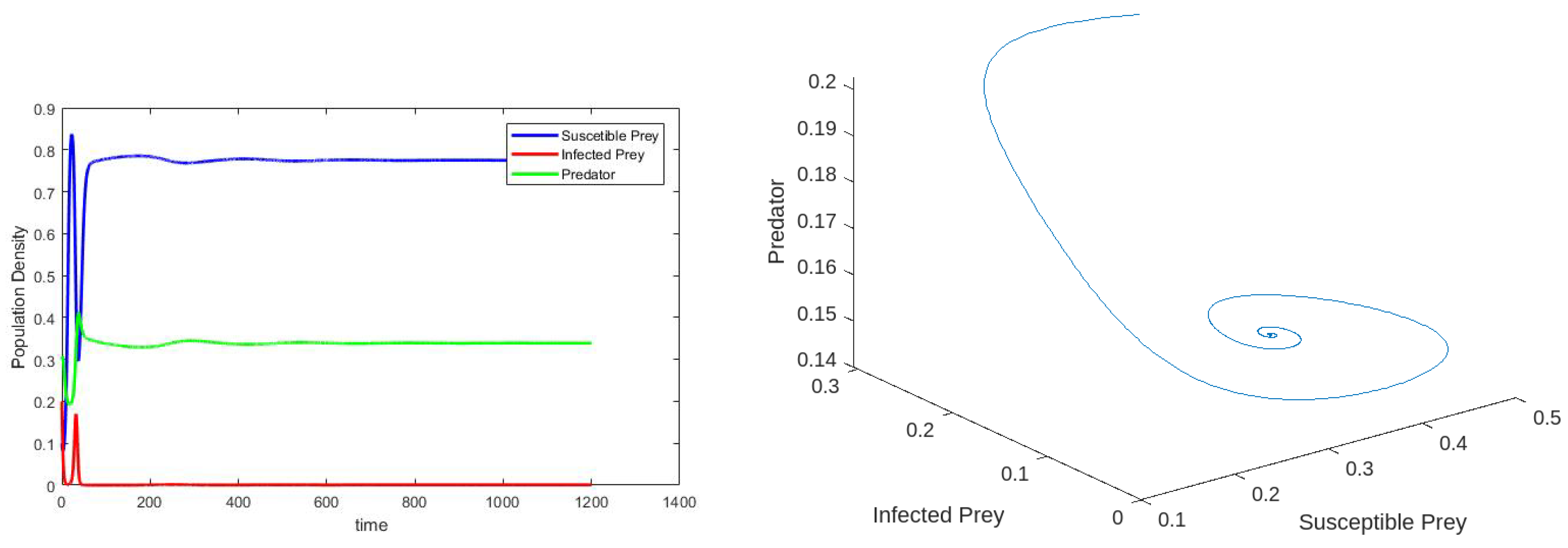
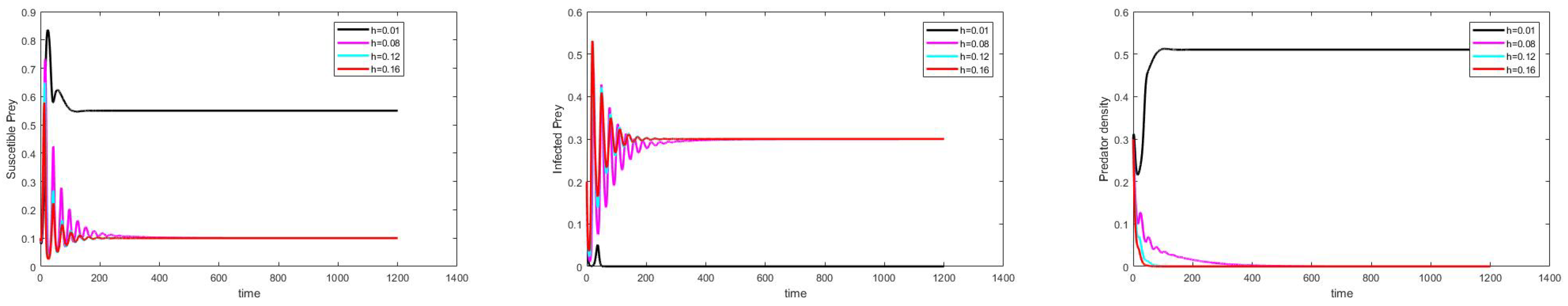
6. Numerical Simulations

In this section, several numerical simulations of the system (Equation (2)) are performed in order to verify the theoretical findings. In the present study, the rate of harvesting $\left(h\right)$ and predation rate $\left(\alpha \right)$ are the key parameters, which will be taken as control parameters. The MATLAB software programme is used to carry out the numerical simulation for the provided set of parameter values.

Effect of Varying the Harvesting Rate h

For the given parametric values, as in

Table 2. Parametric values of the system (Equation (2)).

Parameters	Indicative Number
$\beta$	Variable
$\alpha$	Variable
h	0.1
a	0.2
d	0.6
r	0.3
$\delta$	0.4
c	0.5
$\theta$	0.7

with $\alpha =0.2$, the without predator equilibrium point $E_2$ and the endemic equilibrium point $E^{\ast }$ exist for $0.1<h<0.32$. Figure 1 shows time series for the system (Equation (3)) for $h=0.08$ and phase portrait of the system at $E^{\ast }$. Figure 2 shows susceptible and infected and predator prey population with different values for $h=0.01,0.08,0.2,0.3$. It can be observed that an increase in the harvesting rate of susceptible prey leads to a decrease in the susceptible prey and predator population, but an increase in the infected prey population.

7. Conclusions

In this study, we investigated the three-species food web model in an eco-epidemiological model with predator harvesting. Local stability was assigned to each biologically feasible equilibrium point of the system. Harvesting rate (h) was used as a control parameter. According to the analytical and numerical findings, the harvesting rate has a major impact on the population. Furthermore, increasing the susceptible prey harvesting rate leads to a decrease in the susceptible prey and predator population, but an increase in the infected prey population. If we increase the rate of harvesting in predator populations, the system loses its stability. Also, as we increase the level of harvesting, the system loses its stability and becomes unstable. This study shows the complex behavior of the proposed model.

References

1. Ashwin, A.; Sivabalan, M.; Divya, A.; Siva Pradeep, M. Dynamics of Holling Type II Eco-Epidemiological Model with Fear Effect, Prey Refuge, and Prey Harvesting. Available online: https://sciforum.net/paper/view/14404 (accessed on 25 October 2023).
2. Divya, A.; Sivabalan, M.; Ashwin, A.; Siva Pradeep, M. Dynamics of Ratio Dependent Eco Epidemiological Model with Prey Refuge and Prey Harvesting. Available online: https://sciforum.net/paper/view/14744 (accessed on 25 October 2023).
3. Yue, Q. Dynamics of a modified Leslie-Gower predator-prey model with Holling-type II schemes and a prey refuge. Springerplus 2016, 5, 461. [Google Scholar] [CrossRef] [PubMed]
4. Lavanya, R.; Vinoth, S.; Sathiyanathan, K.; Tabekoueng, Z.N.; Hammachukiattikul, P.; Vadivel, R. Dynamical Behavior of a Delayed Holling Type-II Predator-Prey Model with Predator Cannibalism. J. Math. 2022, 2022, 4071375. [Google Scholar] [CrossRef]
5. Melese, D.; Muhye, O.; Sahu, S.K. Dynamical behavior of an eco-epidemiological model incorporating prey refuge and prey harvesting. Appl. Appl. Math. Int. J. (AAM) 2020, 15, 1193–1212. [Google Scholar]
6. Tripathi, J.P.; Jana, D.; Tiwari, V. A Beddington–DeAngelis type one-predator two-prey competitive system with help. Nonlinear Dyn. 2018, 94, 553–573. [Google Scholar] [CrossRef]
7. Tripathi, J.P.; Abbas, S.; Thakur, M. A density dependent delayed predator–prey model with Beddington–DeAngelis type function response incorporating a prey refuge. Commun. Nonlinear Sci. Numer. Simul. 2015, 22, 427–450. [Google Scholar] [CrossRef]
8. Gunasekaran, N.; Vadivel, R.; Zhai, G.; Vinoth, S. Finite-time stability analysis and control of stochastic SIR epidemic model: A study of COVID-19. Biomed. Signal Process. Control. 2023, 86, 105123. [Google Scholar] [CrossRef] [PubMed]
Figure 1. Time series for the system (Equation (2)) for h = 0.08 and phase portrait of the system at E .
Engproc 56 00124 g001
Figure 2. Susceptible and infected and Predator prey population with different values for h = 0.01 , 0.08 , 0.2 , 0.3 . It can be observed that an increase in the harvesting rate of susceptible prey leads to a decrease in the susceptible prey and predator population, but an increase in the infected prey population.
Engproc 56 00124 g002