Influence of Frequency-Sweep on Discrete and Continuous Phase Distributions Generated in Alkali-Metal Vapours ^†

Abstract

This paper describes a comparable study on the influence of frequency-sweep on the discrete and continuous phase distributions associated with pulse excitations for a double-lambda atomic system in alkali-metal vapours with a hyperfine structure. The excitation dynamics provided a different scheme of sigmoidal types, and the optical pulses were assumed to be Gaussians. We focused on the set-up of electromagnetically induced transparency (EIT). The phases of optical fields show similarities to discrete square wave distributions influenced by ramping. The results showed significant control of discrete phase distributions and temporal ramping by the implementation of sigmoidal membership functions. The relevant equations are the reduced Maxwell equations for the radiation fields, and the density matrix equation in the Liouville space governs the time evolution.

1. Introduction

In recent papers, we have studied the temporal profile associated with the phases of dual-colour pulses, such as the drive and the probe train in a double-lambda system composed of the hyperfine states of alkali atoms with a nuclear spin (I = 3/2) [1,2]. The field’s phases were shown to form temporal discrete distributions such as square waves. The significant parameters were the detuning of the upper hyperfine levels and the atomic radiative relaxations. For this study, we were interested in temporal discrete and continuous phase distributions, which characterize the interaction with time-dependent frequency-sweep for both drive and probe fields. The frequency scanned the splitting of the upper hyperfine levels. The shape of frequency-sweep is given in terms of sigmoidal-type membership functions (SMF) [3]. The benefits of using SMF rely on the fact that it contains two member functions to control the shape of the sigmoid function. In such a way, we aim to manipulate the temporal profile of the field’s phases. Allen and Eberly obtained an analytical solution for two-level Bloch equations and deduced the sech pulse for the field envelope, where they used tanh frequency-sweep [4]. Recently, Kaviani et al. analysed the process of sweeping the resonance frequency of two-level atoms in an adiabatic regime [5]. They showed that the atomic frequency-sweep (AFS) memory has similarities to EIT-based memories in terms of quantum storage and retrieval of light experiments.

The approach proposed in this paper attempts to generalize the foundations of Allen and Eberly [4] to the case of multilevel atoms interacting with polychromatic electromagnetic fields. We further implement dual-frequency frequency-sweep on the optical transitions of the lower-lambda system. This is intended to study their impact on the phases without appealing to the polaritons concept, which was introduced by Fleischhauer and Lukin [6] and applied by Kaviani et al. in the case of sweeping the atomic frequency for quantum storage and retrieval of light [5].

2. The Atomic System and Its Optical Excitation Scheme

In this section, we analyse a double-lambda configuration with a two-colour excitation of ⁸⁷Rb atoms within the D₁ line, i.e., 5s ²S_1/2 − 5p ²P_1/2 [2]. The bar states can be described in terms of the generic four states: |1⟩ = |5 ²S_1/2(F_g = 1)⟩; |2⟩ = |5 ²S_1/2(F_g = 2)⟩; |3⟩ = |5 ²P_1/2(F_e = 1)⟩; and |4⟩ = |5 ²P_1/2(F_e = 1)⟩, where F_g (F_e) stands for the total angular momentum associated with ground and excited hyperfine states. The filed probe was tuned to the transition 1 ↔ 3, and the drive filed was tuned to the transition 2 ↔ 3. The 1 ↔ 2 was a dipole-forbidden transition.

The hyperfine splitting of the ground and excited states is denoted by Δω_g and Δω_e, respectively. The Rabi frequencies for the probe and drive transition are indicated by Ω_p and Ω_r, respectively. In the following section, we consider working in relative units. Ω(Δω) is the Rabi frequency (detuning) in units of γ; the spontaneous decay rate of the excited atomic state, ²P_1/2. The normalized distance ζ and the normalized retarded-time τ were measured in units of the Beers length of one of the pulses and the excited atomic-state lifetime, respectively. We took the spectroscopic data of ⁸⁷Rb from [7]. In the present work, the configuration of the probe-drive was different from the case of chirped stimulated rapid adiabatic passage considered by Chathanathi et al. [8]. We kept only the one-photon detuning as a function of time, while the two-photon detuning was compensated for by the instantaneous chirping of the probe and drive. The one-photon, time-dependent detuning of the probe and drive are defined as:

δ_p(t) = ω_p(t) − ω₃₁,
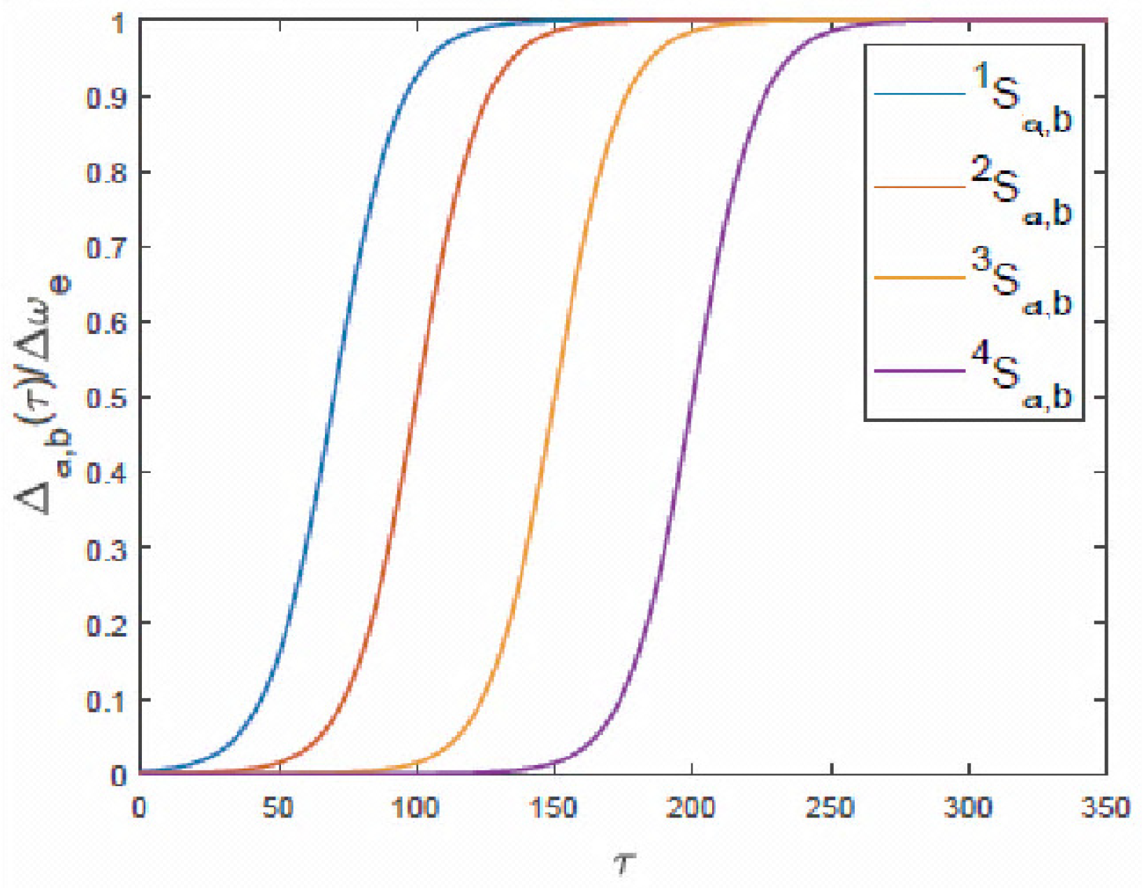
δ_r(t) = ω_r(t) − ω₃₂,

(1)

where ω_p and ω_r stand for the instantaneous angular frequencies of the probe and drive, with the atomic transition angular frequencies ω₃₁ and ω₃₂. We aimed to scan the frequency across the upper hyperfine splitting (Δω_e). We set ω_p(0) = ω₃₁ and ω_r(0) = ω₃₂. The frequency-sweep did not undershoot or overshoot the upper hyperfine splitting. Therefore, the endpoints of the sweep were well-defined, as pointed out by Sawyer et al. [9].

We chose the function S(T, a, b), as in the Matlab sigmoidal membership function [3]. Its first argument T represents the interaction time domain T = [τ₀, τ_f], where τ₀ and τ_f denote the initial and final time which were considered. The function S(T, a, b) contains two membership functions that control the time profile and approach to unity for the final times. Therefore, the frequency-sweep can be rewritten as

δ_p(T, a, b) = Δω_e ∗ S_p(T, a, b),
δ_r(T, a, b) = Δω_e ∗ S_r(T, a, b).

(2)

Finally, the instantaneous sweeping Δ_a,b(τ) can be written as the interpolation of δ(T, a, b) at the moment τ

Δ_a,b(τ) = spline(T, δ(T, a, b), τ).

(3)

Figure 1 presents the frequency-sweep Δ_a,b(τ) as a function of time for different membership functions of the sigmoidal-type excitation.

Figure 2 depicts the chopping of the frequency-sweep function at a constant time step of Δτ = 12.5.

The time evolution of the reduced density matrix ρ_s(t) is given by the first-order Liouville–von Neumann differential equation:

$$-i \frac{\partial {\rho }_s\left(\tau \right)}{\partial t}={\widehat{\mathcal{L}}}_t{\rho }_s(\tau ), \hslash =1,$$

(4)

where ${\widehat{\mathcal{L}}}_t$ stands for the Liouvillian super-operator in the Liouville space [10,11].

The reduced Maxwell equations are related to the two-component polarizations of rank one: ${\rho }_{ \mathrm{3,1}}^{\left(10\right)} , {\rho }_{ \mathrm{4,1}}^{\left(10\right)}$ and ${\rho }_{ \mathrm{3,2}}^{\left(10\right)} , {\rho }_{ \mathrm{4,2}}^{\left(10\right)}$ were associated with probe and drive transitions as follows:

$$\begin{gathered} \frac{\partial }{\partial \zeta }{\mathsf{\Omega }}_p(\zeta , \tau )=\sqrt{8/6}[{\rho }_{\mathrm{3,1}}^{\left(10\right)} (\zeta , \tau )-\sqrt{5}{\rho }_{\mathrm{4,1}}^{(10)} (\zeta , \tau )], \\ \frac{\partial }{\partial \zeta }{\mathsf{\Omega }}_r\left(\zeta , \tau \right)=\sqrt{8/2}\left[{\rho }_{\mathrm{3,2}}^{\left(10\right)} \left(\zeta , \tau \right)-{\rho }_{\mathrm{4,2}}^{\left(10\right)} \left(\zeta , \tau \right)\right], \end{gathered}$$

(5)

where m = 0 for the magnetic quantum number. The probe and drive were linearly polarized and propagated co-linearly.

The time evolution of the density matrix can be described as follows:

$$\frac{\partial }{\partial \tau }\rho (\tau )=L({\Gamma }^k, {\mathsf{\Delta }\omega }_e, {\mathsf{\Delta }\omega }_g{, }^p{\mathsf{\Delta }}_{a,b}(\tau ){,}^{ r}{\mathsf{\Delta }}_{a,b},\frac{{\mathsf{\Omega }}_p}{\sqrt{8}},\frac{{\mathsf{\Omega }}_r}{\sqrt{8}}) \rho (\tau )$$

(6)

where Γ^k represents the relative relaxation rate components of rank k, and L is the Liouvillian matrix [11]. Let ^rΔ_a,b(τ) and ^pΔ_a,b(τ) refer to the time-dependent detuning for the drive and probe, respectively.

3. Numerical Results

Throughout this study, we restricted ourselves to the response of rubidium atoms. Other alkalines, like sodium and potassium, give quite different time-dependent phase distributions, indicating a strong dependence on the upper hyperfine splitting and atomic relaxations. Figure 3 depicts the temporal behaviour of the injected pulses at ζ = 0, with black curves representing the probe and drive. The initial temporal pulse profiles for the probe and drive were assumed to be Gaussian. In this study, we truncated the initial interaction time to contain only two probe fields instead of three, as was carried out in [1,2]. Furthermore, we kept the domain of the time-axis the same. Long-time behaviour manifested the ring field response, yielding significant ramping in the phase distributions. Alhasan et al. discussed the influence of the ring field on the propagation stability of ultra-short pulses in duplicated two-level atom media [12].

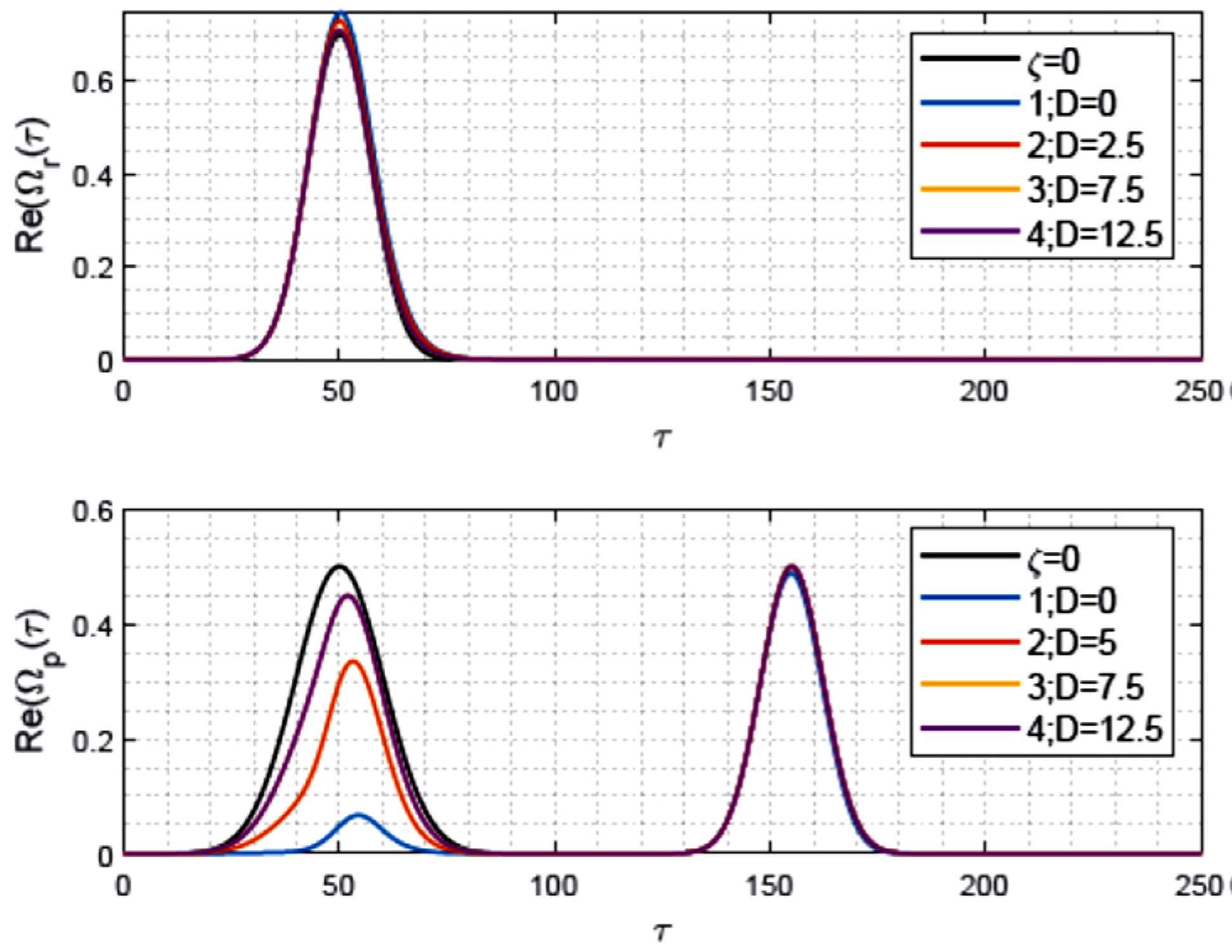
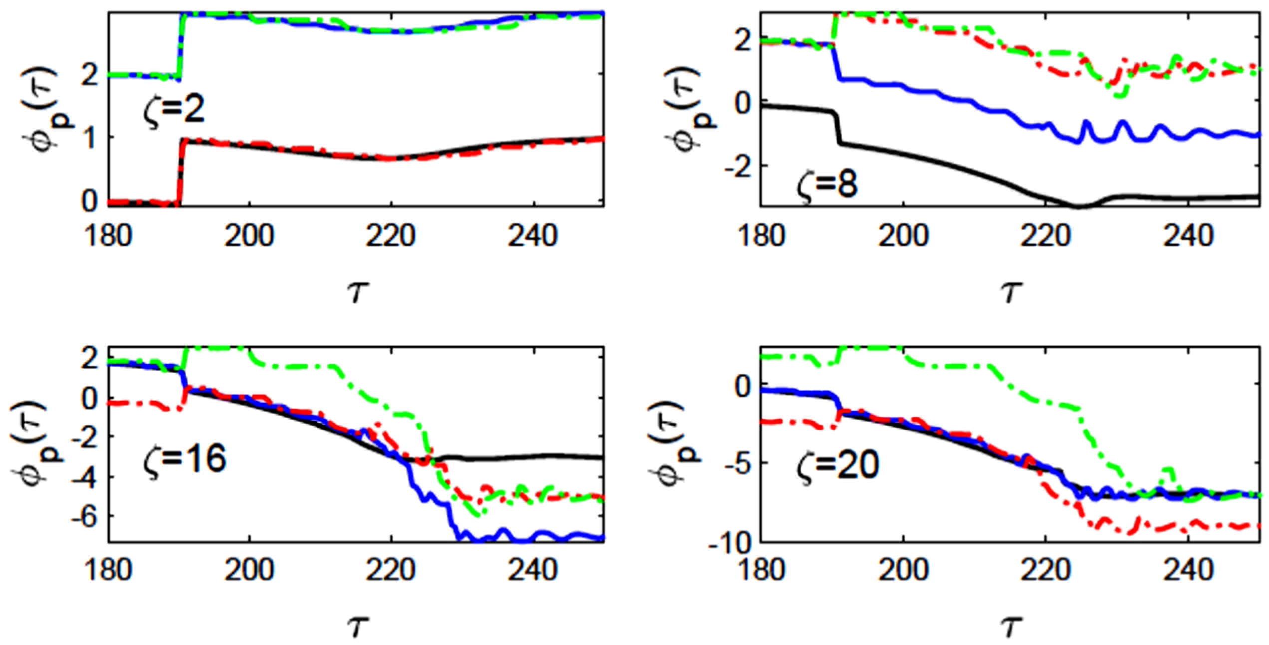
Pulse Profiles, Energy, Phase, and Propagation

Figure 3 shows the temporal pulse profiles of the drive and probe at the final distance considered, ζ = 21. Black curves represent the reference pulses without chirping at ζ = 0.

The effect of sweeping was considered for the third case, with ³S_a,b and ³Δ_a,b showing different chirping, as presented in Figure 3. The drive field maxima at ζ = 21 were close to the injected pulse at ζ = 0. Let us compare the relative energies at ζ = 21 for different chirping frequencies as

[^a₁^,b₁E_r ^a₂^,b₂E_r ^a₃^,b₃E_r ^a₄^,b₄E_r] = [1.0000 1.1031 1.0334 1.0333]

(7)

There was a tendency to increase the energy of the drive pulse as it was frequency-swept off the resonance frequency. There was strong absorption in the first probe pulse, without chirping. The transparency increased as the probe pulsed off-resonantly through chirping. The transparency for the second probe in the train for large swept off-resonances was remarkable. Figure 4 shows enhancements of the imaginary parts of the probe pulses. Such an effect was responsible for the phase production. Let us define the time section T₁(τ) = [0, 180] as the effective duration time of the pulses with the atomic medium, without its tail. The initial interval, T₀(τ) = [0, 70], was omitted since the field response is so small, and the phase took an initial constant value of 0π. For Figure 5, we considered presenting the temporal shapes of the probe train in different phases for different locations inside the medium, and for chopping time intervals: Δτ = 0, 5, 7.5, and 12.5. The discrete phase distributions are evident for small distances, like ζ = 2. The phase jumped to build-up at τ₁ = 100, as the final time required to finish the interaction with the first probe pulses. The second phase’s discontinuity started at τ₂ = 120, and the time was defined as the interaction with the second probe pulse as the train started up. Beyond the second interaction time, the phases remained at constant values, i.e., τ ∈ [120, 180]. In Figure 5a, we distinguish discrete distributions associated with various colours as follows:

1. Black: {0π, −1π, 0π}; with chopping time interval Δτ = 0;

2. Blue: {0π, 1π, 2π}; with chopping time interval Δτ = 5;

3. Red: {0π, 1π, 0π}; with chopping time interval Δτ = 7.5;

4. Green: {0π, 1π, 2π}; with chopping time interval Δτ = 12.5.

Figure 4. The imaginary part of the probe field at distance ζ = 21 for different chopping time intervals. The third case, ³S_a,b and ³Δ_a,b, is considered.

Figure 4. The imaginary part of the probe field at distance ζ = 21 for different chopping time intervals. The third case, ³S_a,b and ³Δ_a,b, is considered.

Figure 5. Phase profile corresponding to interaction time for the probe pulse at different distances, where the effect of sweeping was considered for the third case, ³S_a,b, and ³Δ_a,b at various chopping times. The chopping time intervals were Δτ = 0, 5, 7.5, and 12.5 for the black, blue, red, and green curves, respectively. The panels (a–d) are corresponding to distances ζ = 2, ζ = 8, ζ = 16 and ζ = 20, respectively.

Figure 5. Phase profile corresponding to interaction time for the probe pulse at different distances, where the effect of sweeping was considered for the third case, ³S_a,b, and ³Δ_a,b at various chopping times. The chopping time intervals were Δτ = 0, 5, 7.5, and 12.5 for the black, blue, red, and green curves, respectively. The panels (a–d) are corresponding to distances ζ = 2, ζ = 8, ζ = 16 and ζ = 20, respectively.

For moderate distances, as in Figure 5b, we distinguished the continuous and discrete combinations as follows:

1. Black: {ϵ₁(τ), 0π,−1π, 0π};

2. Red: {0π, −1π, 0π};

3. Green: {ϵ₂(τ), 1π, 2π}.

The function ϵ₁(τ) grew at a small interval, but eventually collapsed to 0π phases, while the function ϵ₂(τ) grew and ended with π values.

In Figure 5d, the blue curve overrides the black curve, leaving distinct limiting cases such as {−2π, 0π, 2π}.

Figure 6 depicts the long-time behaviour of temporal phases as the extended-time response for the ring field after the dominant existence of the pulses. The ring fields exposed phase-ramping through short stepping and yielding phase mutations. Finally, the limiting phases were stabilized. Intermediate chopping time intervals of Δτ = 5 and 7.5 (blue and red curves) defined substantial phases as −7π and −10π, respectively.

4. Conclusions

We discussed the phase response of dual-colour pulse excitation in alkaline vapours with a hyperfine structure. The pulses were similarly frequency-swept within the upper hyperfine splitting. The sweeping excitation was a sigmoidal-type function with two membership functions to control the final time achievement and adjust the sweeping rate. We also analysed the effect of increasing chopping time intervals on phase generation and stabilization within the propagation inside the medium. We calculated the phases for one of the alkaline vapours, namely, rubidium. The distribution of phases was different for different alkaline vapours due to the strong dependence on the upper hyperfine splitting and the atomic relaxation. The numerical results showed that the phases could be categorized into two distinctive distributions: discrete and continuous, with a superposition of discrete or continuous ramping mutations. For a small distance, we obtained two-phase discontinuities. Beyond the discontinuities, the phases maintained constant values. We identified eight phase distributions for different chopping intervals. These distributions were produced over the pulse’s mean length. We also noted another type of phase generated due to the ring field for long-time responses and asymptotic behaviour at long distances. The ring fields exposed phase-ramping through short stepping and producing phase mutations with substantial phases, i.e., −7π and −10π.

References

1. Alhasan, A.M.; Abdulrhmann, S. Multilevel Phase Switch Generation in Alkali Vapors. Eng. Proc. 2023, 31, 69. [Google Scholar]
2. Alhasan, A.M.; Altowyan, A.S.; Madkhli, A.Y.; Abdulrhmann, S. Multiple Phase Stepping Generation in Alkali Metal Atoms: A Comparative Theoretical Study. Appl. Sci. 2023, 13, 3670. [Google Scholar] [CrossRef]
3. Sigmoidal Membership Function. Available online: https://www.mathworks.com/help/fuzzy/sigmf.html (accessed on 27 July 2023).
4. Allen, L.; Eberly, J. Optical Resonance and Two-Level Atoms; Courier Corporation: New York, NY, USA, 1975; pp. 101–104. [Google Scholar]
5. Kaviani, H.; Khazali, M.; Ghobadi, R.; Zahedinejad, E.; Heshami, K.; Simon, K. Quantum storage and retrieval of light by sweeping the atomic frequency. New J. Phys. 2013, 15, 085029. [Google Scholar] [CrossRef]
6. Fleischhauer, M.; Lukin, M.D. Quantum memory for photons: Dark-state polaritons. Phys. Rev. A 2002, 65, 022314. [Google Scholar] [CrossRef]
7. Steck, D.A. Rubidium 87 D Line Data. (Version 2.2.2, Last Revised 9 July 2021). Available online: http://steck.us/alkalidata (accessed on 27 July 2023).
8. Chathanathil, J.; Ramaswamy, A.; Malinovsky, V.S.; Budker, D.; Malinovskaya, S.A. Chirped Fractional Stimulated Raman Adiabatic Passage. Phys. Rev. A 2023, 108, 043710. [Google Scholar] [CrossRef]
9. Sawyer, B.J.; Chilcott, M.; Thomas, R.; Deb, A.B.; Kjærgaard, N. Deterministic quantum state transfer of atoms in a random magnetic field. Eur. Phys. J. D 2019, 73, 160. [Google Scholar] [CrossRef]
10. Fiutak, J.; van Kranendonk, J. The effect of collisions on resonance fluorescence and Rayleigh scattering at high intensities. J. Phys. B At. Mol. Phys. 1980, 13, 2869–2884. [Google Scholar] [CrossRef]
11. Alhasan, A.M. Entropy Associated with Information Storage and Its Retrieval. Entropy 2015, 17, 5920–5937. [Google Scholar] [CrossRef]
12. Alhasan, A.M.; Czub, J.; Miklaszewski, W. Propagation of light pulses in a (j1 = 1/2) ↔ (j2 = 1/2) medium in the sharp-line limit. Phys. Rev. A 2009, 80, 033809. [Google Scholar] [CrossRef]
Figure 1. The frequency-sweep function Δa,b(τ) along with the course of time for different membership functions a and b with the following assessments: 1, a = 0.0841, b = 70; 2, a = 0.0841, b = 100; 3, a = 0.0841, b = 150; 4, a = 0.0841, b = 200.
Engproc 56 00161 g001
Figure 2. The chopped frequency-sweep function cΔa,b(τ) along with the course of time for different membership functions a and b with the following assessments: 1, a = 0.0841, b = 70; 2, a = 0.0841, b = 100; 3, a = 0.0841, b = 150; 4, a = 0.0841, b = 200. The chopping time interval was Δτ = 12.5.
Engproc 56 00161 g002
Figure 3. Drive and probe temporal pulse profiles of the drive and probe. Black curves correspond to the reference pulses without chirping at ζ = 0, and various colours correspond to the final distance at ζ = 21. The effect of sweeping was considered for the third case, with 3Sa,b and 3Δa,b at different time-chopping steps: D = Δτ = 0, 5, 7.5, and 12.5.
Engproc 56 00161 g003
Figure 6. Extended-time phase profile for the probe pulse at different distances, where the effect of sweeping was considered for the third case, 3Sa,b, and 3Δa,b at various chopping times. The chopping time intervals were Δτ = 0, 5, 7.5, and 12.5 for the black, blue, red, and green curves, respectively.
Engproc 56 00161 g006
Disclaimer/Publisher’s Note: The statements, opinions and data contained in all publications are solely those of the individual author(s) and contributor(s) and not of MDPI and/or the editor(s). MDPI and/or the editor(s) disclaim responsibility for any injury to people or property resulting from any ideas, methods, instructions or products referred to in the content.