Dynamical Analysis of a Fractional Order Prey–Predator Model in Crowley–Martin Functional Response with Prey Harvesting ^†

Abstract

In this paper, we investigate a fractional-order predator–prey model incorporating prey harvesting. In a non-delayed model, the Crowley–Martin functional response is studied. We first prove the existence, uniqueness, non-negativity and boundedness of the solutions for the proposed model. Furthermore, the existence of various equilibrium points is analyzed to examine the local asymptotically stable properties, and the suitable Lyapunov function is used to study the globally asymptotic stability. Finally, some numerical simulations are verified for the analytic results.

1. Introduction

Fractional calculus (FC) is a general field that attempts to understand real-world phenomena. A non-integer sequence is modeled with derivatives and is a field of differentiation and integrations are performed with non-integer order derivatives. The memory impact and conserved relevant physical properties are the benefits of fractional derivatives. The predator–prey models developed by Lotka and Voltera are considered to be early developments in contemporary mathematical ecology in a coupled system of nonlinear differential equations [1,2]. Since Kermack-Mckendrick’s pioneering work on SIRS, epidemiological models have attracted much interest from researchers [3]. In general, there are two main types of mathematical models: ecological and epidemiological models. The relations between the populations of a certain community are explored in ecological models [4]. Epidemiology models are studies of how illnesses spread between humans and animals. This article’s major objective is to investigate how infection affects prey during prey harvesting in a predator–prey system. Here, we examined the local and global stabilities of the equilibrium points of this system, as well as the boundedness and positivity of the solution [5,6]. An eco-epidemiological predator–prey system with disease affecting only prey species and the harvesting of both susceptible and infected prey has been taken into consideration by Bhattacharya et al. [7,8]. Agnihotri and Gakkhar studied a prey–predator system with disease affecting both species and only the prey species being harvested [9,10]. The SIRS-type models are mathematically similar to models of the s-called geometric Brownian motion (GBM): both predict an exponential growth of infected individuals or of the value of the process. The state of dead individuals in the SIRS models is akin to the so-called resetting in the GBM model [11,12]. The very relevant model of GBM with resetting was recently considered in refs. Ecologists, economists, and those involved in natural resource management were interested in the studies on harvesting in predator–prey systems for some time. A few people have specifically included a harvested parameter in a predator–prey–parasite model and analyzed the system’s response to it [13]. In this article, we examine the function of harvesting in an eco-epidemiological system where susceptible and diseased prey are harvested together [14,15]. This study applies the Caputo fractional derivative and the harvesting rate to the predator–prey model. This author’s major objective is to investigate the effects of prey infection and prey harvesting in a predator–prey system. Here, we examined the boundedness, positivity, local and global stabilities, and stability of the system’s equilibrium points.

2. Model Formulation

The model explains how the diseased prey system interacts with harvesting, which results in the following set of equations. The dynamic prey and predator mathematical model was investigated using the proposed model,

$$\left.\begin{array}{c}\frac{dL}{dT}=r_{1}L(1-\frac{L+M}{K})-\lambda ML-\frac{{\alpha }_{1}LN}{(1+\zeta L)(1+\eta N)}-H_1{E}_{1}L,\hfill \\ \frac{dM}{dT}=\lambda ML-d_{1}M-\frac{b_{1}MN}{a_1+M}-H_2{E}_{2}M,\hfill \\ \frac{dN}{dT}=-d_{2}M+\frac{c{b}_{1}MN}{a_1+M}+\frac{c{\alpha }_{1}LN}{(1+\zeta L)(1+\eta N)}.\hfill \end{array}\right\}$$

(1)

Subject to initial conditions $L\left(0\right)\ge 0$, $M\left(0\right)\ge 0$, $N\left(0\right)\ge 0$.

The detailed biological meanings of parameters are given in

Table 1. Biological representation of the system (1) parameters.

Parameters	Biological Representation
L	Susceptible prey
M	Infected prey
N	Predator
$r_1$	Intrinsic prey growth rate
K	Carrying capacity of the environment
${\alpha }_1$	Predation rate of susceptible prey
$b_1$	Predation rate of infected prey
$a_1$	Half-saturation constant
c	Conversion coefficient from the prey to predator
$d_1$	Infected prey death rate
$d_2$	Predator population death rate
$\lambda$	Infection rate

.

The variables $l=\frac{L}{K}$, $m=\frac{M}{K}$, $n=\frac{N}{K}$ and the dimension time $t=\lambda KT$ can be changed in order to reduce the number of parameters in the system (1). We apply the following transformations

$$\begin{array}{c}\hfill s_1=\frac{r_1}{\lambda k},s_2=\frac{{\alpha }_1}{\lambda K},s_3=\frac{a_1}{k},s_4=\frac{{\alpha }_1}{\lambda K},s_5=\frac{b_1}{\lambda k},s_6=\frac{d_2}{\lambda k}.\end{array}$$

To the above transformations, Equation (1) can be rewritten in the following non-dimensional form

$$\left.\begin{array}{cc}{\displaystyle \frac{dl}{dt}=s_{1}l(1-l-m)-lm-\frac{s_{2}ln}{(1+\zeta l)(1+\eta n)}-{\theta }_{1}l,}\hfill & \\ {\displaystyle \frac{dm}{dt}=lm-s_{4m}-\frac{s_{5}mn}{s_3+m}-{\theta }_{2}m,}\hfill & \\ {\displaystyle \frac{dn}{dt}=-s_{6}n+\frac{c{s}_{5}mn}{s_3+m}+\frac{c{s}_{2}ln}{(1+\zeta l)(1+\eta n)}.}\hfill \end{array}\right\}$$

(2)

Subject to initial conditions $l\left(0\right)\ge 0$, $m\left(0\right)\ge 0$, $n\left(0\right)\ge 0$.

We have taken fractional-order derivative $\alpha$ to model (2) with restore the fractional-order Caputo derivative. Then, the model (2) is take into the following form

$$\left.\begin{array}{cc}{\displaystyle \frac{d^{\alpha }l}{d{t}^{\alpha }}=s_{1}l(1-l-m)-lm-\frac{s_{2}ln}{(1+\zeta l)(1+\eta n)}-{\theta }_{1}l,}\hfill & \\ {\displaystyle \frac{d^{\alpha }m}{d{t}^{\alpha }}=lm-s_{4}m-\frac{s_{5}mn}{s_3+m}-{\theta }_{2}m,}\hfill & \\ {\displaystyle \frac{d^{\alpha }n}{d{t}^{\alpha }}=-s_{6}n+\frac{c{s}_{5}mn}{s_3+m}+\frac{c{s}_{2}ln}{(1+\zeta l)(1+\eta n)}.}\hfill \end{array}\right\}$$

(3)

subject to the initial conditions $l\left(0\right)\ge 0$, $m\left(0\right)\ge 0$, $n\left(0\right)\ge 0$.

3. Existence and Uniqueness of the Solutions

In this section, the boundedness of the solution of the system (3) was examined. The fractional-order system as follows:

$$\begin{array}{cc}\hfill {\displaystyle \frac{d^{\alpha }X\left(t\right)}{{dt}^{\alpha }}}& \hfill =f(t,X(t\left)\right),\alpha \in (0,1].\hfill \end{array}$$

Theorem 1. 

The fractional-order system (3) has a unique solution for the non-negative initial conditions.

Proof. 

A sufficient condition for the solutions of system (3) in the region $\chi \times (0,T]$,

$$\chi =\left\{(l,m,n)\in R^3:max\left(\right|l|,|m|,|n\left|\right)\le \eta \right\}.$$

Let us define a mapping $V\left(X\right)=(V_1\left(X\right),V_2\left(X\right),V_3\left(X\right))$

$$\begin{array}{cc}{V}_1\left(X\right)& {\displaystyle =s_{1}l(1-l-m)-lm-\frac{s_{2}ln}{(1+\zeta l)(1+\eta n)}-{\theta }_{1}l,}\hfill \\ V_2\left(X\right)& {\displaystyle =lm-s_{4}m-\frac{s_{5}mn}{s_3+m}-{\theta }_{2}m,}\hfill \\ V_3\left(X\right)\hfill & {\displaystyle =-s_{6}n+\frac{c{s}_{5}mn}{s_3+m}+\frac{c{s}_{2}ln}{(1+\zeta l)(1+\eta n)}.}\hfill \end{array}$$

$$\begin{array}{cc}\left|\right|V\left(X\right)-V\left(\overline{X}\right)\left|\right|& = |V_1\left(X\right)-V_1\left(\overline{X}\right)| + |V_2\left(X\right)-V_2\left(\overline{X}\right)| + |V_3\left(X\right)-V_3\left(\overline{X}\right)|\hfill \\ & {\displaystyle = |s_{1}l(1-l-m)-lm-\frac{s_{2}ln}{(1+\zeta l)(1+\eta n)}-{\theta }_{1}l-s_1\overline{l}(1-\overline{l}-\overline{m})+\overline{l}\overline{m}}\hfill \\ & {\displaystyle +\frac{s_2\overline{l}\overline{m}}{(1+\zeta \overline{l})(1 + \eta \overline{n})} + {\theta }_1\overline{l}| + |lm-s_{4}m-\frac{s_{5}mn}{s_3+m}-{\theta }_{2}m-\overline{l}\overline{m}+s_4\overline{m}}\hfill \\ & {\displaystyle +\frac{s_5\overline{m}\overline{n}}{s_3+\overline{m}}+{\theta }_2\overline{m}| + |-s_{6}n+\frac{c{s}_{5}mn}{s_3+m}+\frac{c{s}_{2}ln}{(1+\zeta l)(1+\eta n)}+s_6\overline{n}-\frac{c{s}_5\overline{m}\overline{n}}{s_3+\overline{m}}}\hfill \\ & {\displaystyle -\frac{c{s}_2\overline{l}\overline{n}}{(1+\zeta \overline{l})(1+\eta \overline{n})}|}\hfill \\ & \le \left\{s_1+2s_1\eta +(2+s_1\eta )+(1+c)\eta s_2{s}_3+{\theta }_1\right\}\left|l-\overline{l}\right|\hfill \\ & +\left\{s_1\eta +(1+c)s_5\eta +s_4+{\theta }_2\right\}\left|m-\overline{m}\right|\hfill \\ & +\left\{(1+c)s_2{s}_3\eta +(1+c)s_2{s}_3{\eta }^2+(1+c)s_5\eta +s_6\right\}\left|n-\overline{n}\right|\hfill \\ & \le H∥X-\overline{X}∥.\hfill \end{array}$$

where, $H=max\left\{{\displaystyle s_1+2s_1\eta +(2+s_1)\eta +\frac{(1+c)s_2{s}_3\eta }{{(s_2+\eta )}^2}+{\theta }_1,(s_1+s_5+c{s}_5)\eta +s_4+{\theta }_2}\right.$

$\left.{\displaystyle \frac{(1+c)s_2{s}_3\eta }{{(s_3+\eta )}^2}+\frac{(1+c)s_2{s}_3{\eta }^2}{{(s_3+\eta )}^2}+(1+c)s_5\eta +s_6}\right\}$

Hence, the solution of the system (3) exists and is unique. □

4. Equilibrium Points and Stability Analysis

In this section, the system (3) has the following possible equilibrium points:

(i)

The trivial equilibrium point is $E_0(0, 0, 0)$.

(ii)

$E_1\left({\displaystyle \frac{s_1-{\theta }_1}{s_1}, 0, 0}\right)$ is the boundary equilibrium point.

(iii)

$E_2(\overline{l}, 0 ,\overline{n})$ is the infected prey free equilibrium point, where ${\displaystyle \overline{l}=\frac{s_6(1+\eta n)}{c{s}_2-s_6\zeta (1+\eta n)}}$,

${\displaystyle \overline{n}=\frac{s_1(1-l)(1+\zeta l)}{s_2+{\theta }_1-\eta s_1(1-l)(1+\zeta l)}}$.

(iv)

$E_3(\widehat{l}, \widehat{m}, 0)$ is the predator free equilibrium point, where $\widehat{l}=s_4+{\theta }_2$,

${\displaystyle \widehat{m}=\frac{s_1(1-s_4-{\theta }_2)-{\theta }_1}{s_1+1}}$.

(v)

The interior equilibrium point $E^{*}(l^{*}, m^{*}, n^{*})$. Where,

$$\begin{array}{c}\hfill {\displaystyle m^{*}=\frac{s_3(s_3{s}_6+(s_6-c{s}_2)l^{*})}{(c{s}_2{l}^{*}+(c{s}_5-s_6)(1+\zeta l^{*})},n^{*}=\frac{s_{3}c(l^{*}+s_4-{\theta }_2)(1+\zeta l^{*})}{(c{s}_2{l}^{*}+(c{s}_5-s_6)((1+\eta n^{*})}}\end{array}$$

and $l^{*}$ is the unique positive root of the quadratic equation $A{l}^2+Bm+C=0$ where $A=s_1(c{s}_2+c{s}_5-s_6)$, $B=(c{s}_5-s_6)({\theta }_1-s_1+s_3{s}_1)+s_{3}c({\theta }_1-s_1)+s_3(s_6+(s_6-c{s}_1)s_1)$, $C=-s_3((s_1-{\theta }_1)(c{s}_5-s_6)+(c{s}_2(s_4+{\theta }_2)-s_3{s}_4(1+s_1))$.

Now, we want to calculate the Jacobian matrix for a local stability analysis around different equilibrium points. The Jacobian matrix at an arbitrary point $(l,m,n)$ is given by

$$J(l,m,n)=\left(\begin{array}{ccc}{n}_{11}& n_{12}& n_{13}\\ n_{21}& n_{22}& n_{23}\\ n_{31}& n_{32}& n_{33}\end{array}\right).$$

where, ${\displaystyle n_{11}=s_1(1-2l)-m(s_1+1)-\frac{s_{2}n}{{(1+\zeta l)}^2(1+\eta n)}-{\theta }_1,n_{12}=-l(s_1+1)}$,

${\displaystyle n_{13}=-\frac{s_{2}l}{(1+\zeta l){(1+\eta n)}^2}}$, $n_{21}=m$, ${\displaystyle n_{22}=l-s_4-{\theta }_2-\frac{s_3{s}_{5}n}{{(s_3+m)}^2}}$, ${\displaystyle n_{23}=\frac{s_{5}m}{s_3+m}}$,

${\displaystyle n_{31}=\frac{c{s}_{2}n}{{(1+\zeta l)}^2(1+\eta n)}}$, ${\displaystyle n_{32}=\frac{s_{3}c{s}_{5}n}{{(s_3+m)}^2}}$, ${\displaystyle n_{33}=-s_6+\frac{c{s}_{5}m}{s_3+m}+\frac{s_{2}cl}{(1+\zeta l){(1+\eta n)}^2}}$.

Theorem 2. 

The trivial equilibrium point $E_0(0,0,0)$ of a system (3) is stable if $s_1<{\theta }_1$; otherwise, it is unstable.

Proof. 

The Jacobian matrix of the system (3) at an equilibrium point $E_0$ is given by

$$J\left(E_0\right)=\left(\begin{array}{ccc}{s}_1-{\theta }_1& 0& 0\\ 0& -s_4-{\theta }_2& 0\\ 0& 0& -s_6\end{array}\right).$$

Here, eigenvalues are ${\lambda }_1=s_1-{\theta }_1$, ${\lambda }_2=-s_4-{\theta }_2$ and ${\lambda }_3=-s_6$.

Hence, the trivial equilibrium point $E_0(0,0,0)$ is stable if $s_1<{\theta }_1$, otherwise, it is unstable. □

Theorem 3. 

The infected free and predator free equilibrium point ${\displaystyle E_1(\frac{s_1-{\theta }_1}{s_1}, 0, 0)}$ of a system (3) is stable if $c{s}_2(s_1-{\theta }_1)<s_6(s_1+\zeta (s_1-{\theta }_1))$.

Proof. 

The Jacobian matrix of the system (3) at an equilibrium point $E_1$ is given by

$$J\left(E_1\right)=\left(\begin{array}{ccc}{\theta }_1-s_1& -\left({\displaystyle \frac{s_1-h_1}{s_1}}\right)(s_1+1)& {\displaystyle \frac{-s_2(s_1-{\theta }_1)}{s_1{s}_3+(s_1-{\theta }_1)}}\\ 0& {\displaystyle 1-s_4-{\theta }_2-\frac{{\theta }_1}{s_1}}& 0\\ 0& 0& {\displaystyle \frac{-s_2(s_1-{\theta }_1)}{s_1{s}_3+(s_1-{\theta }_1)-s_6}}\end{array}\right).$$

Here, eigenvalues are ${\lambda }_1={\theta }_1-s_1$, ${\displaystyle {\lambda }_2=1-s_4-{\theta }_2-\frac{{\theta }_1}{s_1}}$ and ${\displaystyle {\lambda }_3=\frac{-s_2(s_1-{\theta }_1)}{s_1{s}_3+(s_1-{\theta }_1)-s_6}}$.

Hence, the infected prey and predator free equilibrium point $E_1$ is stable. □

Theorem 4. 

The disease free equilibrium point $E_2$ of a system (3) is locally asymptotically stable if $min\left\{{\displaystyle \frac{s_3{s}_6}{c-s_6}-s_4,s_1\left({\displaystyle 1-\frac{2s_3{s}_6}{c-s_6}}\right)}\right\}<{\theta }_1$.

Proof. 

$J\left(E_2\right)=$$\left(\begin{array}{ccc}{d}_{11}& d_{12}& d_{13}\\ d_{21}& d_{22}& d_{23}\\ d_{31}& d_{32}& d_{33}\end{array}\right)$ where, ${\displaystyle d_{11}=-{\theta }_1+s_1-\frac{2s_3{s}_1{s}_6}{c{s}_2-s_6}-\frac{{(c{s}_2-s_6)}^2\overline{n}}{s_3{s}_2{c}^2}}$, ${\displaystyle d_{12}=-\frac{s_3(1+s_1)s_6}{c-s_6}}$, ${\displaystyle d_{13}=-\frac{s_6}{c}}$,

$d_{21}=0$, ${\displaystyle d_{22}=-s_4-{\theta }_2+\frac{s_3{s}_6}{c{s}_2-s_6}}$, $d_{23}=0$, ${\displaystyle d_{31}=\frac{\left({(c{s}_2-s_6)}^2\overline{n}\right)}{s_{3}c{s}_2}}$, ${\displaystyle d_{32}=\frac{c{s}_5\overline{n}}{s_3}}$, $d_{33}=0.$

Here, the characteristic equation of the above Jacobian matrix is

$$\begin{array}{c}\hfill {\lambda }^3+P{\lambda }^2+Q\lambda +R=0.\end{array}$$

(4)

where $P=-p_{11}-p_{22}$, $Q=-p_{31}{p}_{13}+p_{22}{p}_{11}$, $R=p_{13}{p}_{12}{p}_{31}$.

According to the Routh–Hurwitz criteria [16], $P>0$, $R>0$, and $PQ-R>0$.

Hence, $E_2$ is locally asymptotically stable. □

Theorem 5. 

The equilibrium point $E_3$ of a system (3) is locally asymptotically stable if $s_6>c(s_2+s_5)$.

Proof. 

The Jacobian matrix at $E_3$ is given by

$$J\left(E_3\right)=\left(\begin{array}{ccc}{m}_{11}& m_{12}& m_{13}\\ m_{21}& m_{22}& m_{23}\\ m_{31}& m_{32}& m_{33}\end{array}\right).$$

where $m_{11}=-(s_4+{\theta }_2)s_1$, $m_{12}=(-1-s_1)\overline{l}$, ${\displaystyle m_{13}=\frac{-s_2}{{(1+\zeta l)}^2)(1+\eta n)}}$, $m_{21}=m$,

$m_{22}=0$, $m_{23}=\frac{s_5\overline{m}}{s_3+\overline{m}}$, $m_{31}=0$, $m_{32}=0$, and $m_{33}=\frac{c{s}_2\overline{l}}{(1+\zeta l){(1+\eta n)}^2}-s_6+\frac{c{s}_5\overline{m}}{s_3+m}$.

Here, the characteristic equation of the above Jacobian matrix is

$$\begin{array}{c}\hfill {\lambda }^3+E{\lambda }^2+F\lambda +G=0.\end{array}$$

(5)

where $E=-m_{11}-m_{33}$, $F=-m_{21}{m}_{12}+m_{33}{m}_{11}$, $G=m_{12}{m}_{21}{m}_{33}$.

According to the Routh–Hurwitz criteria [16], $E>0$, $G>0$, and $EF-G>0$.

Hence, $E_3$ is locally asymptotically stable. □

Theorem 6. 

The endemic equilibrium point $E^{*}$ of system (3) is locally asymptotically stable.

Proof. 

The Jacobian matrix at $E^{*}$ is given by

$$J\left(E^{*}\right)=\left(\begin{array}{ccc}{g}_{11}& g_{12}& g_{13}\\ g_{21}& g_{22}& g_{23}\\ g_{31}& g_{32}& g_{33}\end{array}\right).$$

where $g_{11}=s_1(1-2l^{*})-m(s_1+1)-\frac{s_{2}n}{{(1+\zeta l^{*})}^2(1+\eta n^{*})}-{\theta }_1$, $g_{12}=-l^{*}(s_1+1)$,

$g_{13}=-\frac{s_2{l}^{*}}{(1+\zeta l^{*}){(1+\eta n^{*})}^2}$, $g_{21}=m^{*}$, $g_{22}=l^{*}-s_4-{\theta }_2-\frac{s_3{s}_5{n}^{*}}{{(s_3+m^{*})}^2}$, ${\displaystyle g_{23}=\frac{s_5{m}^{*}}{s_3+m^{*}}}$,

${\displaystyle g_{31}=\frac{c{s}_2{n}^{*}}{{(1+\zeta l^{*})}^2(1+\eta n^{*})}}$, ${\displaystyle g_{32}=\frac{s_{3}c{s}_5{n}^{*}}{{(s_3+m^{*})}^2}}$, ${\displaystyle g_{33}=-s_6+\frac{c{s}_5{m}^{*}}{s_3+m^{*}}+\frac{s_{2}c{l}^{*}}{(1+\zeta l^{*}){(1+\eta n^{*})}^2}}$.

Here, the characteristic equation of the above Jacobian matrix is

$$\begin{array}{c}\hfill {\lambda }^3+E{\lambda }^2+F\lambda +G=0.\end{array}$$

(6)

where $E=-g_{11}-g_{33}$, $F=g_{21}{g}_{12}+g_{22}{g}_{11}-g_{13}{g}_{31}+g_{23}{g}_{32}$, $G=g_{13}(-g_{22}{g}_{31}+g_{21}{g}_{32})+g_{23}(g_{12}{g}_{31}-g_{11}{g}_{32})$.

According to the Routh-Hurwitz criteria [16], $E>0$, $G>0$, and $EF-G>0$.

Hence, $E^{*}$ is locally asymptotically stable. □

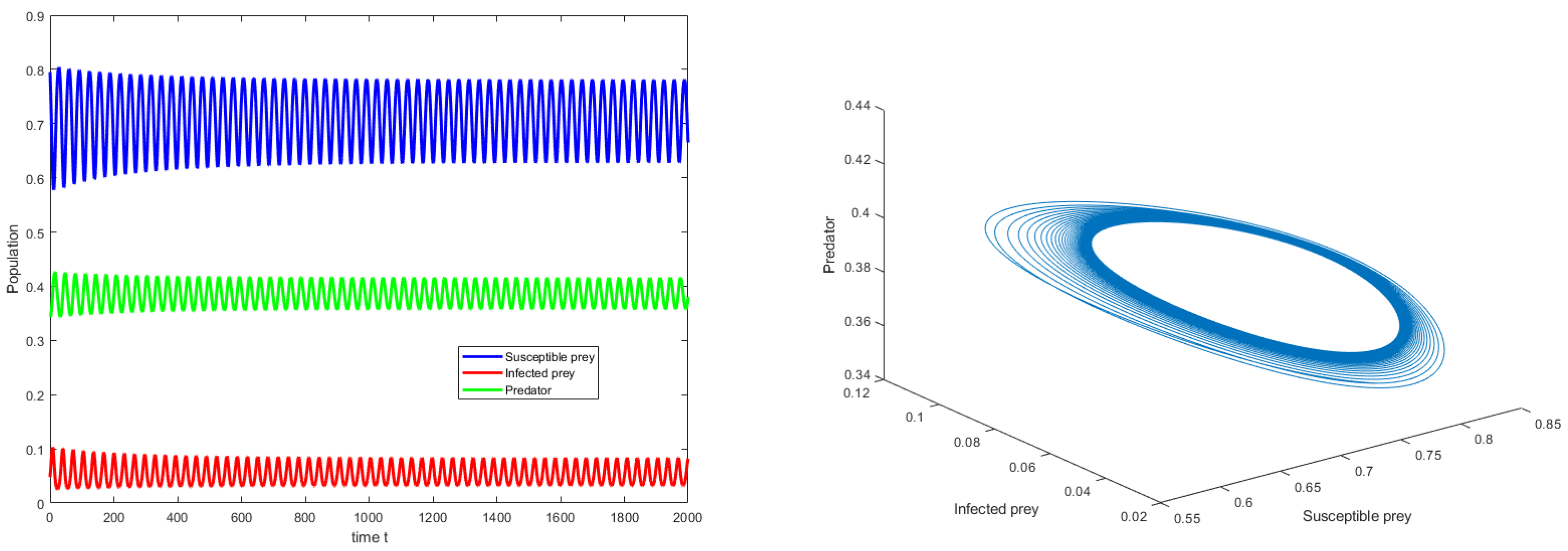
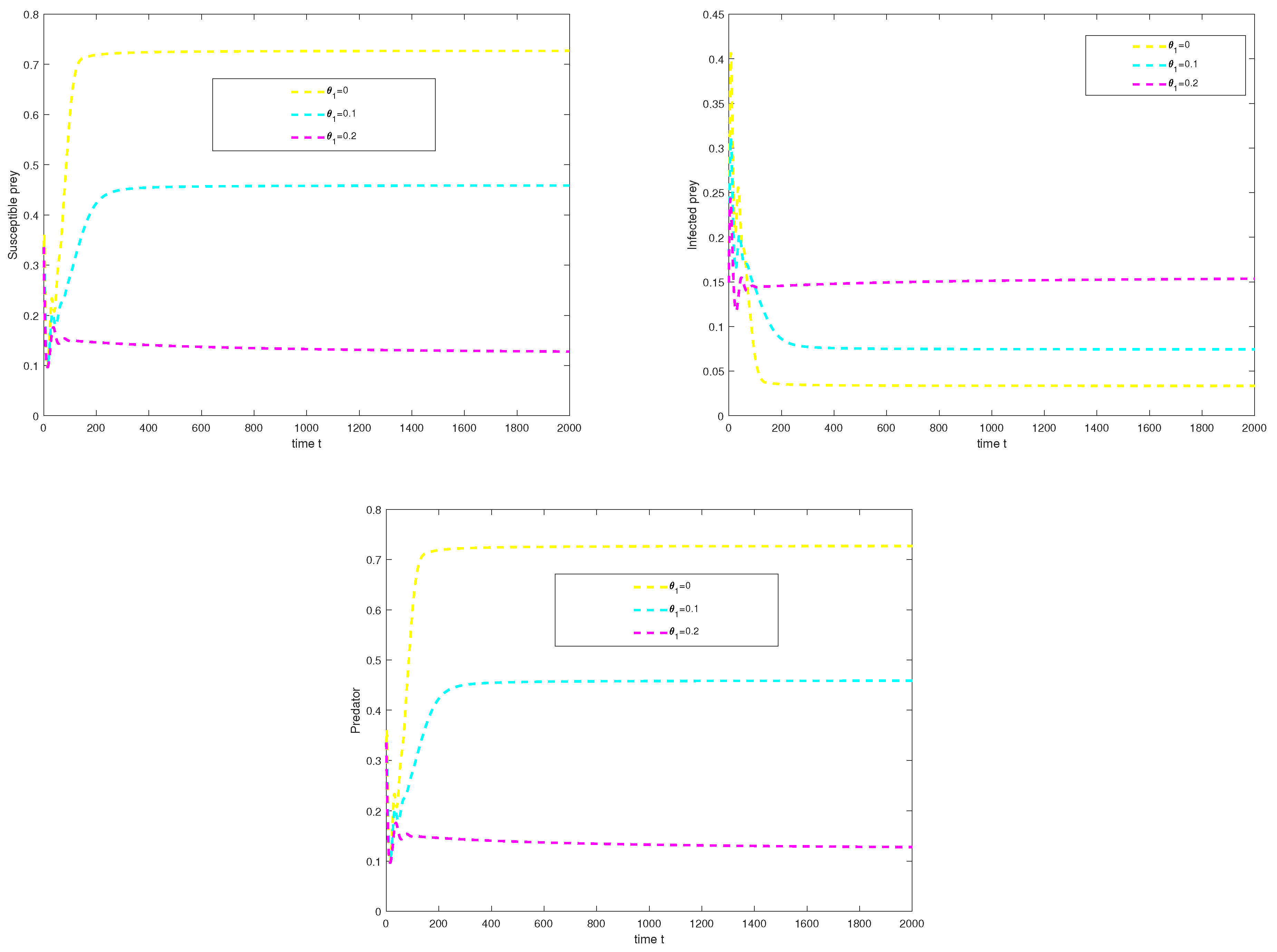
5. Numerical Analysis

In this section, we present some numerical simulation results for the Caputo-sense fractional-order eco-epidemic models. To accomplish this, we use Diethelm et al.’s predictor–corrector approach to solve the defined model. The parameter values are chosen as $s_1=0.5$, $s_2=0.15$, $s_3=0.2$, $s_4=0.1$, $s_5=0.4$, $s_6=0.1$, $c=0.5$, $\zeta =0.5$, $\eta =0.3$, and the different values of $\alpha =1$ and then the equilibrium point $E_4(0.794787,0.0476298,0.343099)$ are unstable (see Figure 1). Fixing the derivative $\alpha$ as a variable. Here, we consider the derivative value as $\alpha =0.92$, and the effect of the predator harvesting ${\theta }_1$ on the evolution of the three species clearly influences the final size of the three populations, as shown in Figure 2.

6. Conclusions

In this study, we investigated a fractional-order derivative-based model of a three-species food web. Each equilibrium point’s local stability in our proposed fractional-order system has also been examined. The suggested mathematical model’s numerical simulation results show that the proposed system changes from unstable to stable as the order of the fractional derivative’s value, $\alpha$, goes from 0 to 1. It is obvious that for the different values of $\alpha$ in the range $0<\alpha <1$, the unstable system with the integer-order $\alpha =1$ becomes a stable system. For the interior equilibrium point, when the derivative of $\alpha =1$, the system becomes unstable, and if we change the order to fractional order, $\alpha =0.92$, and the system becomes stable. When the susceptible prey population harvesting rate increases, then the infected prey population harvesting rate decreases in the fractional order derivative. Since the susceptible prey population is inversely proportional to the infected prey population in the system, then the derivative of the fractional-order alpha makes an important contribution to the proposed system’s dynamical stability.

References

1. Lotka, A.J. Elements of Physical Biology; Williams & Wilkins: Philadelphia, PA, USA, 1925. [Google Scholar] [CrossRef]
2. Volterra, V. Variazioni e Fluttuazioni del Numero d’Individui in Specie Animali Conviventi; Societa Anonima Tipografica “Leonardo da Vinci”: Citta di Castello, Italy, 1926. [Google Scholar] [CrossRef]
3. Kermack, W.O.; McKendrick, A.G. A contribution to the mathematical theory of epidemics. Proc. R. Soc. Lond. Ser. Contain. Pap. Math. Phys. Character 1927, 115, 700–721. [Google Scholar] [CrossRef]
4. Ashwin, A.; Sivabalan, M.; Divya, A.; Siva Pradeep, M. Dynamics of Holling type II eco-epidemiological model with fear effect, prey refuge and prey harvesting. In Proceedings of the 1st International Online Conference on Mathematics and Applications, online, 1–15 May 2023; MDPI: Basel, Switzerland, 2023. [Google Scholar]
5. Panigoro, H.S.; Suryanto, A.; Kusumawinahyu, W.M.; Darti, I. Dynamics of an eco-epidemic predator–prey model involving fractional derivatives with power-law and Mittag–Leffler kernel. Symmetry 2021, 13, 785. [Google Scholar] [CrossRef]
6. Ramesh, P.; Sambath, M.; Mohd, M.H.; Balachandran, K. Stability analysis of the fractional-order prey-predator model with infection. Int. J. Model. Simul. 2021, 41, 434–450. [Google Scholar] [CrossRef]
7. Ahmed, E.; El-Sayed, A.M.; El-Saka, H.A. Equilibrium points, stability and numerical solutions of fractional-order predator–prey and rabies models. J. Math. Anal. Appl. 2007, 325, 542–553. [Google Scholar] [CrossRef]
8. Stojkoski, V.; Sandev, T.; Kocarev, L.; Pal, A. Geometric Brownian motion under stochastic resetting: A stationary yet nonergodic process. Phys. Rev. E 2021, 104, 014121. [Google Scholar] [CrossRef]
9. Yang, W. Dynamical behaviors of a diffusive predator–prey model with Beddington–DeAngelis functional response and disease in the prey. Int. J. Biomath. 2017, 10, 1750119. [Google Scholar] [CrossRef]
10. Divya, A.; Sivabalan, M.; Ashwin, A.; Siva Pradeep, M. Dynamics of Ratio dependent eco epidemiological model with prey refuge and prey harvesting. In Proceedings of the 1st International Online Conference on Mathematics and Applications, online, 1–15 May 2023; MDPI: Basel, Switzerland, 2023. [Google Scholar]
11. Burov, S.; Jeon, J.H.; Metzler, R.; Barkai, E. Single particle tracking in systems showing anomalous diffusion: The role of weak ergodicity breaking. Phys. Chem. Chem. Phys. 2011, 13, 1800–1812. [Google Scholar] [CrossRef]
12. Metzler, R.; Jeon, J.H.; Cherstvy, A.G.; Barkai, E. Anomalous diffusion models and their properties: Non-stationarity, non-ergodicity, and ageing at the centenary of single particle tracking. Phys. Chem. Chem. Phys. 2014, 16, 24128–24164. [Google Scholar] [CrossRef]
13. Vinod, D.; Cherstvy, A.G.; Wang, W.; Metzler, R.; Sokolov, I.M. Nonergodicity of reset geometric Brownian motion. Phys. Rev. E 2022, 105, L012106. [Google Scholar] [CrossRef] [PubMed]
14. Das, M.; Maiti, A.; Samanta, G.P. Stability analysis of a prey-predator fractional order model incorporating prey refuge. Ecol. Genet. Genom. 2018, 7–8, 33–46. [Google Scholar] [CrossRef]
15. Mondal, S.; Lahiri, A.; Bairagi, N. Analysis of a fractional order eco-epidemiological model with prey infection and type 2 functional response. Math. Methods Appl. Sci. 2017, 40, 6776–6789. [Google Scholar] [CrossRef]
16. Murray, J.D. Mathematical Biology I: An Introduction; Springer: Berlin/Heidelberg, Germany, 2002. [Google Scholar] [CrossRef]
Figure 1. Unstable solution for the interior equilibrium point α = 1 .
Engproc 56 00300 g001
Figure 2. It is varying the harvesting rate of susceptible prey, infected prey, and a predator population with different values of θ 1 = 0 , 0.1 , 0.2 for the fractional-order derivative α = 0.92 .
Engproc 56 00300 g002